A dynamic simulation approach to identify
additional reactive reserves against long-term
voltage instability
Lampros Papangelis
Dept. of Elec. Eng. and Comp. Science University of Li`ege, Belgium
Patrick Panciatici
Marie-Sophie Debry
RTE, R & D dept. Versailles, France
Thierry Van Cutsem
Fund for Scientific Research (FNRS) at University of Li`ege, Belgium
Abstract—A simple method is proposed to identify additional reactive reserves enabling to counteract long-term voltage insta-bility after a large disturbance. In contrast to the many references based on power flow calculations, the method resorts to dynamic simulation. The post-disturbance system evolution is simulated in the presence of time-varying shunt susceptances with specified rate of change. This allows to deal with dynamic issues such as the required speed of the additional reactive power sources, or the onset of unstable electromechanical oscillations. Furthermore, a compromise is sought between the speed of action and the volume of additional compensation. The method is demonstrated on a detailed model of the Nordic test system.
Index Terms—long-term voltage stability, reactive power re-serves, generator capability, load tap changers, time simulation
I. INTRODUCTION
With higher power transfers from renewable generation sites, such as large wind parks, to load centers, the existing transmission systems will be subject to power flows for which they were not designed. Hence, they will be exposed to a higher risk of instability following large disturbances. Among them, voltage instability following the loss of generation or transmission facilities, is often identified as a major threat.
Voltage stability is classified into short- and long-term [1]. The former has to do mainly with the re-acceleration of induction motors after a fault, inducing delayed voltage recovery, and in unstable cases, motor stalling. In long-term voltage instability, the initial outage and the generator reactive power limitations decrease the maximum power deliverable to loads below the level that the latter tend to restore [2].
One way of strengthening a system against voltage insta-bility consists of increasing its reactive reserves, hosted by reactive power sources reacting automatically to disturbances [2]. While counteracting short-term voltage instability requires fast reactive power sources, such as static var compensators or static compensators, it is generally considered that long-term voltage instability can be counteracted by (the less expensive) switching of shunt compensation. There is, however, a minimal speed at which this compensation must be brought into service, in order the system to regain an equilibrium [2]. Other issues to consider are the cascade tripping of equipment by
protections reacting to low voltages, or the onset of growing electromechanical oscillations.
A very large number of publications deal with the optimal location and size (and, to some extent, type) of those additional reactive power sources [3]. A majority of them are based on power flow calculations, thus neglecting the post-disturbance dynamics of the system. An optimal power flow is generally solved to find the compensation scheme that optimizes some objective [4]. The more recent references [5]–[9] have incor-porated dynamic aspects, mainly in the context of short-term voltage instability.
This paper focuses on a simple method to determine where, how much and how fast additional reactive power should be injected to counteract long-term voltage instability after a major disturbance. This information is obtained by running a modified dynamic simulation of the system subject to the disturbance of concern, and supported by shunt compensation devices with a specified rate of time variation, mimicking the way compensation would be activated in post-disturbance conditions. Time simulation allows taking into account dy-namic issues such as attraction towards a final equilibrium, cascade tripping of components, or the onset of unstable electromechanical oscillations.
Furthermore, although the method is not claimed to yield an “optimal” reactive compensation, a simple procedure is proposed to find a compromise between the speed of action and the volume of the additional compensation.
The rest of the paper is organized as follows. Section II presents the model of the additional reactive power sources. Section III illustrates their performance on the Nordic test sys-tem and shows the information retrieved from time simulation. A procedure to achieve a smaller compensation is presented in Section IV. Concluding remarks are offered in SectionV.
II. MODELLING AND BEHAVIOUR OF COMPENSATION
A. Time-varying shunt compensation
The proposed method resorts to Time-varying Shunt Sus-ceptances (TSS) placed at various candidate locations and injecting reactive power to counteract the system degradation triggered by the initial disturbance and developing under
TSS near generator ˙ B 1 s
˜
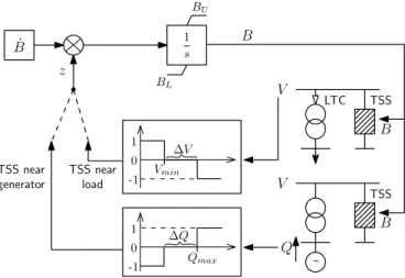
B LTC B Q z TSS TSS TSS near load B BL BU V V 1 0 Vmin ∆V -1 1 0 Qmax -1 ∆QFigure 1. Model of the Time-varying Shunt Susceptance (TSS)
the effect of Load Tap Changers (LTCs) and OverExcitation Limiters (OELs) [2].
The simple model of each TSS is shown in Fig. 1. B is the variable susceptance related to the injected reactive power by:
Q= BV2 (1)
˙
B is the specified rate of variation in time of B. By varying the value of ˙B, different speeds of action against the system degra-dation are achieved. As far as long-term voltage instability is concerned, it can be shown that slower corrective actions may have to be larger in magnitude to restore attraction towards an equilibrium [2]. Therefore, it can be expected that a value
˙
B is suitable for one contingency, but inadequate for a more severe one. Moreover, it is possible that even very high values of ˙B cannot save the system against a contingency. Those cases usually relate to other forms of instability, of short-term nature, for which shunt compensation is not appropriate.
The variable z in Fig. 1 is an integer with z∈ {−1, 0, 1}. It takes the value1 when reactive power must be injected into the grid, and −1 when it has to be withdrawn from the grid. Initially, the TSS is inactive with B = 0 and z = 0. With z = 1, the shunt susceptance B increases linearly with time at the rate ˙B, while with z = −1 it decreases at that rate. When the system reaches a steady-state, z gets back to zero and, hence, B remains constant.
The lower limit BL on the (non-windup) integrator is set
to zero in this study, as the emphasis is on under-voltage situations where the TSS must inject reactive power. Extension to BL <0 is straightforward. The choice of the upper limit
BU will be discussed in Section IV. If this limit is reached,
other TSS are expected to take over, but may fail doing so if the limitation is severe.
The z switching logic is also depicted in Fig. 1. Two cases are considered, according to the TSS location, as detailed next. B. TSS near load
A TSS located near a load is activated when the transmis-sion voltage falls below a threshold value Vmin. Due to the
integral control, if the system reaches a new steady state, the
transmission voltage will be restored by the TSS to (at least) Vmin. The choice of this value may obey various criteria. One
of them is to hold the transmission voltage high enough so that the distribution voltages can be restored at their set-points by the LTCs, i.e. the LTCs do not hit their limits and the loads are served at normal voltages. The corresponding value of Vmin
can be computed assuming the distribution transformer ratio at its limit and the distribution voltage still restored to its set-point; a small security margin should be added.
It is possible that the combined actions of all TSS results in too high final voltages. To avoid such overcompensation, a small deadband ∆V is introduced on each TSS, as shown in Fig. 1. Thus, if the voltage rises above Vmin + ∆V , B
is decreased at the rate − ˙B, until the voltage returns in the deadband (or the BL limit is hit).
C. TSS near generator
For a TSS of this second type, the objective is to prevent a nearby generator from getting limited, thereby losing its voltage control ability [10]. It is well known that generator reactive power limitations reduce the maximum power that can be delivered to loads, which is the root cause of long-term voltage instability [2]. Keeping generators under voltage control may be critical also for small-disturbance angle stabil-ity. It also avoids generator voltage drops that could lead to their tripping by under-voltage protections.
Thus, the activation of a TSS of this type relies on the monitoring of the reactive power Q produced by the nearby assigned generator. This is shown in the lowest part of Fig. 1, where z switches from zero to one when Q becomes larger than Qmax. The latter is set somewhat below the limit given
by the generator capability curves. As for the other TSS, z returns to zero when Q gets back below Qmax. This is where
the value of ˙B also plays a role. Indeed, either the TSS reactive injection is fast enough to prevent the limiter from acting, or the machine excitation is temporarily limited.
Furthermore, to avoid unnecessary generator relief, a small ∆Q deadband is introduced, such that, if the TSS has been previously activated (i.e. z has switched from0 to 1) and the generator production Q falls below Qmax− ∆Q, the TSS will
withdraw part of its reactive power injection until Q returns in the deadband (or the BL limit is hit).
In case the generator is tripped, the TSS cannot act since there is no longer a reactive power to monitor. One option is to switch to a voltage-based activation logic, similar to that of the TSS near a load.
III. ILLUSTRATIVE EXAMPLES OFTSSPERFORMANCE
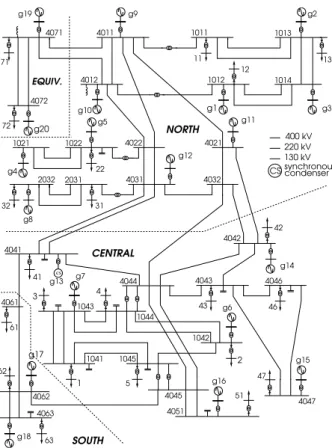
In this section, the operation of the TSS is demonstrated with illustrative examples using the Nordic test system, cur-rently investigated by the IEEE PES Task Force on Test Systems for Voltage Stability and Security Analysis. The variant considered is documented in [11]. Its one-line diagram is shown in Fig. 2. It includes 74 buses and 20 synchronous machines modeled with their excitation systems, OELs, Power System Stabilizers (PSS), turbines and speed governors. The
g15 g11 g20 g19 g16 g17 g18 g2 g6 g7 g14 g13 g8 g12 g4 g5 g10 g1 g3 g9 4011 4012 1011 1012 1014 1013 1022 1021 2031 cs 4046 4043 4044 4032 4031 4022 4021 4071 4072 4041 1042 1045 1041 4063 4061 1043 1044 4047 4051 4045 4062 400 kV 220 kV 130 kV synchronous condenser CS NORTH CENTRAL EQUIV. SOUTH 4042 2032 41 1 5 3 2 51 47 42 61 62 63 4 43 46 31 32 22 11 13 12 72 71
Figure 2. Nordic test system
voltage-dependent loads are represented behind distribution transformers equipped with LTCs reacting with various delays. The insecure operating point A, detailed in [11], has been considered, with a high power transfer from North to Central areas. A number of contingencies can lead to long-term voltage instability, mainly outages of lines in the North-Central corridor or generators in the Central or South areas. The long-term simulations were performed using the RAMSES software developed at the Univ. of Li`ege [12].
TSS were placed in a “brute force” manner at all trans-mission buses near generators and loads. However, as will be shown later, only a small number of them spontaneously react. The so reinforced system was simulated with ˙B set to respectively 1, 2, 4 and 10 Mvar/s. For TSS near loads, the parameter Vmin was set to 0.885 pu with the objective
of bringing distribution voltages back in their deadbands. In case of a generator outage, the TSS previously assigned to it injects reactive power to prevent the transmission voltage of its connection bus from dropping by more than 0.05 pu.
The first contingency considered is the tripping of line 4021-4042 in the North-Central corridor. Without countermeasures, it leads eventually to system collapse in less than 150 s, as shown in Fig. 3. With ˙B set to1 Mvar/s, the system collapse is only delayed, while setting ˙B to 2 Mvar/s is enough to stabilize the system, even in a smooth manner, as shown in Fig. 3.
An overview of the added compensation is provided in Table I. When setting ˙B to 2 Mvar/s, it is found that only
seven TSS react. They are located near generators g5, g7, g8, g10, g11, g12 and g14. For ˙B = 4 and 10 Mvar/s, that number decreases to five, the TSS located near g7 and g10 remaining inactive. The total reactive power added at the final, stabilized operating point, i.e.limt→∞
∑
iBi(t), is reported in
the table. The results confirm the already mentioned property that a faster action requires less effort than a slower one.
Table I
OVERVIEW OFTSSOPERATION IN RESPONSE TO TWO DISTURBANCES
Reactive injection outage line 4021-4042 outage gener. g17
(Mvar at nominal B˙ (Mvar/s) B˙ (Mvar/s)
voltage) 2 4 10 2 4 10 limt→∞∑iBi(t) 944 892 704 - 1323 1148 ∑ imaxt Bi(t) 1305 1026 727 - 1529 1203 Nb of TSS reacting 7 5 5 - 8 7 Nb of TSS with parti- 5 5 5 - 6 6
cipation at final point
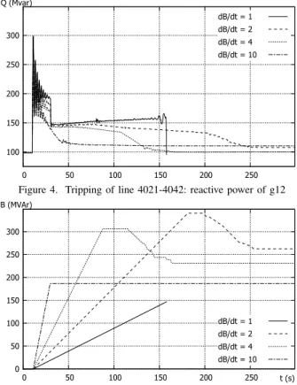
The impact of the TSS speed is further illustrated in Figs. 4 and 5, showing the time evolution of the reactive power generated by g12 and the susceptance of its assigned TSS. For
˙
B= 1 Mvar/s, the system collapses before the TSS succeeds resetting the machine under voltage control. For ˙B = 2 and
˙
B= 4 Mvar/s the machine is temporarily limited, but system collapse is avoided and the machine eventually resets under voltage control. Finally, for ˙B = 10 Mvar/s, the field current overload is alleviated before the OEL acts.
The maximum reactive power transiently injected by each TSS has been recorded, and their sum ∑imaxt Bi(t) is
reported in Table I. It can be seen that a fraction of the added compensation was redundant, and withdrawn before reaching steady state. This can be checked in Fig. 6 for the TSS attached to generator g14. For ˙B= 2 and ˙B= 4 Mvar/s, an overshoot of respectively90 and 70 Mvar is observed, while for ˙B= 10 Mvar/s, the steady-state value is reached without overshoot.
The second contingency is the outage of generator g17. The system is simulated for the same ˙B values and the voltage evolution at bus 1041 is shown in Fig. 7. Setting ˙B to 2 Mvar/s does not yield an acceptable response, since the system eventually experiences unstable electromechanical oscillations. This is attributable to a number of PSS being by-passed by the OELs, which are of the takeover type [2], [11]. By making the TSS faster, voltage control is regained, allowing the PSS to act. For ˙B = 4 Mvar/s, six TSS are active in the final, stabilized steady state, while eight have reacted during the simulation. For ˙B = 10 Mvar/s, those figures become seven and six, respectively. The values of limt→∞
∑
iB(t) and
∑
imaxt Bi(t) (see Table I) indicate that this contingency
is significantly more severe.
From the extensive analysis of other disturbances, the fol-lowing observations were made:
• some disturbances, such as the outage of line
0.75 0.8 0.85 0.9 0.95 1 0 50 100 150 200 250 t (s) V (pu) dB/dt = 0 dB/dt = 1 dB/dt = 2 dB/dt = 4 dB/dt = 10
Figure 3. Tripping of line 4021-4042: voltage at bus 1041
100 150 200 250 300 0 50 100 150 200 250 Q (Mvar) dB/dt = 1 dB/dt = 2 dB/dt = 4 dB/dt = 10
Figure 4. Tripping of line 4021-4042: reactive power of g12
0 50 100 150 200 250 300 350 400 450 0 50 100 150 200 250 t (s) B (Mvar) dB/dt = 1 dB/dt = 2 dB/dt = 4 dB/dt = 10
Figure 5. Tripping of line 4021-4042: susceptance of TSS next to g12
0 50 100 150 200 250 300 0 50 100 150 200 250 t (s) B (MVAr) dB/dt = 1 dB/dt = 2 dB/dt = 4 dB/dt = 10
Figure 6. Tripping of line 4021-4042: susceptance of TSS next to g14
0.75 0.8 0.85 0.9 0.95 1 0 50 100 150 200 250 t (s) V (pu) dB/dt = 0 dB/dt = 1 dB/dt = 2 dB/dt = 4 dB/dt = 10
Figure 7. Outage of generator g17: voltage at bus 1041
by shunt compensation. Even high ˙B values are unable to stabilize the system, and other emergency control schemes have to be contemplated;
• in all stabilized cases, only TSS located near generators
reacted. Furthermore, if TSS were placed near loads only, some disturbances were not corrected (unless the voltage threshold Vmin was set unacceptably high). Thus, in
this system, the dominant cause of voltage instability to address is the lack of reactive reserves. This is expected to hold true in networks with “uniformly” spread gener-ators, leading to rather short electrical distances between generation and load centers.
IV. REFINEMENT OF THE COMPENSATION SCHEME
When designing a shunt compensation scheme, it is desir-able to seek:
• the minimal speed of action, since a fast response may
require to resort to more expensive power-electronics based devices, or may affect power quality;
• the minimal amount of reactive power, since it directly
impacts the cost but also other aspects such as the space available in switching stations.
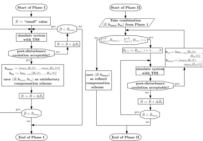
As shown previously, both objectives are conflicting. Searching for a single optimal solution would require weight-ing the respective costs of compensation speed and amount, which is beyond the scope of this paper. The focus here is rather on proposing a set of compensation schemes that yield acceptable system responses. To this purpose, a two-phase procedure is proposed, as described hereafter. The corresponding flow charts are shown in Fig. 8.
A. Phase I
After identifying a harmful contingency, a number N of TSS are placed at candidate locations near loads and/or generators. The system is simulated for various values of ˙B, without limit BU on the TSS (see Fig. 1) and with B initialized
to zero. For simplicity, the same value of ˙B is used in all TSS. The idea is to start from a low ˙B value and increase it by steps of ∆ ˙B1 up to a maximum ˙Bmax. For a given ˙B
value, if the system response is acceptable, the maximum value Bmax= maxt B(t) of each TSS susceptance is recorded, as
well its final steady-state value Bss = limt→∞B(t). If the
response is not acceptable, ˙B is increased and the procedure is repeated, until ˙B > ˙Bmax. The outcome of this phase is
˙ B:= “small” value simulate system with TSS post-disturbance evolution acceptable? ˙ B < ˙Bmax yes yes ˙ B:= ˙B+ ∆ ˙B1 no no
save( ˙B; bmax; bss) as satisfactory
compensation scheme yes no ˙ B:= ˙B+ ∆ ˙B1 ˙ B < ˙Bmax End of Phase I Start of Phase I bss:= limt→∞[B1(t), ..., BN(t)]
bmax:= [maxtB1(t), ..., maxtBN(t)]
PN i=1Bmax,i− PN i=1Bss,i> ǫ yes BU,i:= Bss,i i= 1, . . . , N simulate system with TSS post-disturbance evolution acceptable? yes save( ˙B; bmax) as refined compensation scheme no ˙ B:= ˙B+ ∆ ˙B2 ˙ B < ˙Bmax End of Phase II no no yes Take combination ( ˙B,bmax; bss) from Phase 1
Start of Phase II
bss:= limt→∞[B1(t), . . . ,
BN(t)]
bmax:= [maxtB1(t), . . . ,
maxtBN(t)]
Figure 8. The two phases of the algorithm to refine the shunt compensation scheme
a set of satisfactory compensation schemes, each denoted as ( ˙B, bmax, bss), where bmax(resp. bss) is the vector of Bmax
(resp. Bss) values recorded for all TSS.
B. Phase II
In Phase I, the amount of needed compensation is set to the maximum value reached during the simulation, which is often larger than the final steady-state value. Phase II aims at determining whether this excess susceptance can be spared, while still stabilizing the system. Thus, Phase II translates each scheme ( ˙B, bmax, bss) provided by Phase I into a scheme
( ˙B, bmax), in which the maximum susceptance of each TSS
is fully utilized in the final steady state, i.e.:
Bss,i= Bmax,i, i= 1, . . . , N (2)
It takes as input an initial compensation scheme produced by Phase I for a value of ˙B. If the total maximum compensation exceeds the total steady-state compensation by more than a tolerance ϵ, i.e. N ∑ i=1 Bmax,i− N ∑ i=1 Bss,i> ϵ (3)
the upper limit BU of each TSS is set to its previously reached
steady-state value Bss, and a new simulation is performed
(with B initialized to zero). If an acceptable response is obtained, the aforementioned difference is checked again. If
the system response becomes unacceptable under the effect of the more constraining limit BU, ˙B is increased by a step∆ ˙B2
and a new simulation is performed (unless ˙B > ˙Bmax). The
procedure is repeated until an acceptable response is achieved. Whenever the test (3) is satisfied, the procedure stops and the currently reached compensation scheme( ˙B, bmax) is the
sought output. Then another compensation scheme stemming from phase I can be analyzed.
At this point, it has to be stressed that the ”optimality” of the results is not guaranteed by the algorithm. Instead, it is possible that further reducing the total reactive power of the TSS could still provide an acceptable response, especially for higher values of ˙B. Moreover, the method pays more attention to generators that are operating closer to their reactive limits; the corresponding TSS will always appear in the compensation scheme, although it might not be necessary. Thus, the result of Phase II could be used as the starting point of a search aimed at further refining the compensation scheme. This possibility has not been further considered to preserve the simplicity of the method.
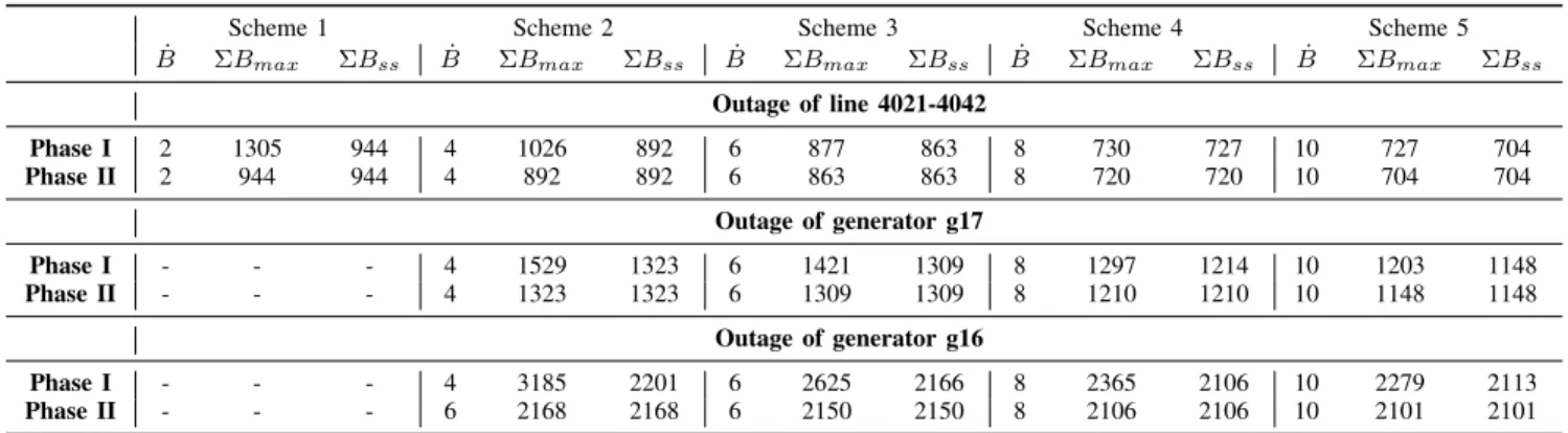
C. Illustrative examples
A sample of representative results of the proposed two-phase procedure is given in Table II. They relate to three dif-ferent contingencies. In Phase I, ˙B values have been scanned up to ˙Bmax = 10 Mvar/s, with a step ∆ ˙B1 = 2 Mvar/s. In
Table II
APPLICATION OF THE TWO-PHASE REFINEMENT ALGORITHM TO THREE CONTINGENCIES
˙
Bis in Mvar/s. ΣBmaxstands for ∑N
i=1Bmax,i and ΣBssfor ∑Ni=1Bss,i. Both are in Mvar.
Scheme 1 Scheme 2 Scheme 3 Scheme 4 Scheme 5
˙
B ΣBmax ΣBss B˙ ΣBmax ΣBss B˙ ΣBmax ΣBss B˙ ΣBmax ΣBss B˙ ΣBmax ΣBss
Outage of line 4021-4042 Phase I 2 1305 944 4 1026 892 6 877 863 8 730 727 10 727 704 Phase II 2 944 944 4 892 892 6 863 863 8 720 720 10 704 704 Outage of generator g17 Phase I - - - 4 1529 1323 6 1421 1309 8 1297 1214 10 1203 1148 Phase II - - - 4 1323 1323 6 1309 1309 8 1210 1210 10 1148 1148 Outage of generator g16 Phase I - - - 4 3185 2201 6 2625 2166 8 2365 2106 10 2279 2113 Phase II - - - 6 2168 2168 6 2150 2150 8 2106 2106 10 2101 2101
tolerance ϵ has been set to 10 Mvar. The resulting sets of compensation schemes are described in Table II by the values of ˙B,∑Ni=1Bmax,iand∑Ni=1Bss,i, respectively.
Generally, it can be seen that the total reactive power needed decreases as ˙B is increased, although the gain becomes less significant for larger values of this parameter.
It was found that, in most cases, limiting the susceptance of the TSS to the final steady-state value does not destabilize a previously stabilized system evolution. The exception was for the tripping of generator g16 with ˙B= 4 Mvar/s. In that case, the transient overshoot of the TSS compensation was indispensable to restore attraction to an equilibrium. Phase II revealed that, after limiting the TSS susceptances, ˙B had to be increased to 6 Mvar/s (since the values 4.5, 5 and 5.5 Mvar/s also failed) in order to achieve an acceptable system response. This yields Scheme 2 in Table II. A separate run of Phase II starting from ˙B = 6 Mvar/s resulted in Scheme 3. However, it can be seen that the difference between both schemes is 18 Mvar, which is negligible.
V. CONCLUSION
A dynamic simulation approach has been presented to identify reactive reserves able to counteract long-term voltage instability after a large disturbance.
A simple technique of time-varying shunt susceptances in-jecting reactive power at various selected locations, in response to the system degradation has been introduced to emulate the activation of shunt compensation devices responding to degraded post-disturbance conditions. The effect of the speed at which reactive power is injected has been demonstrated through illustrative examples on a test system for voltage stability. Moreover, an iterative procedure has been described, which aims at decreasing the amount of compensation while adjusting its speed of action to guarantee the system stabiliza-tion. The outcome of this procedure is a set of satisfactory compensation schemes.
Envisaged future work will deal with:
• the possibility to arbitrate between pre- and
post-disturbance injection of reactive power;
• the extension to short-term dynamics, more precisely the
improvement of voltage recovery after a fault;
• the generalization of the approach to a multiple
contin-gency framework, aiming to identifying a single com-pensation scheme that effectively preserves the system against a whole set of harmful contingencies.
REFERENCES
[1] P. Kundur, J. Paserba, V. Ajjarapu, G. Andersson, A. Bose, C. Canizares, N. Hatziargyriou, D. Hill, A. Stankovic, C. Taylor, T. Van Cutsem, and V. Vittal, “Definition and classification of power system stability IEEE/CIGRE joint task force on stability terms and definitions,” IEEE Transactions on Power Systems, vol. 19, pp. 1387–1401, Aug 2004. [2] T. Van Cutsem and C. Vournas, Voltage stability of electric power
systems, vol. 441. Springer, 1998.
[3] W. Zhang, F. Li, and L. Tolbert, “Review of reactive power planning: Objectives, constraints, and algorithms,” IEEE Transactions on Power Systems, vol. 22, pp. 2177–2186, Nov 2007.
[4] F. Capitanescu, J. M. Ramos, P. Panciatici, D. Kirschen, A. M. Mar-colini, L. Platbrood, and L. Wehenkel, “State-of-the-art, challenges, and future trends in security constrained optimal power flow,” Electric Power Systems Research, vol. 81, no. 8, pp. 1731 – 1741, 2011.
[5] A. Tiwari and V. Ajjarapu, “Optimal allocation of dynamic var support using mixed integer dynamic optimization,” IEEE Transactions on Power Systems, vol. 26, pp. 305–314, Feb 2011.
[6] A. Meliopoulos, V. Vittal, J. McCalley, V. Ajjarapu, and I. Hiskens, “Optimal allocation of static and dynamic var resources,” PSERC, Atlanta, GA, Final Project Report, 2008.
[7] S. Wildenhues, J. Rueda, and I. Erlich, “Optimal allocation and sizing of dynamic var sources using heuristic optimization,” IEEE Transactions on Power Systems, vol. PP, no. 99, pp. 1–9, 2014.
[8] M. Paramasivam, A. Salloum, V. Ajjarapu, V. Vittal, N. Bhatt, and S. Liu, “Dynamic optimization based reactive power planning to mitigate slow voltage recovery and short term voltage instability,” in PES General Meeting — Conference Exposition, 2014 IEEE, July 2014.
[9] H. Liu, V. Krishnan, J. McCalley, and A. Chowdhury, “Optimal planning of static and dynamic reactive power resources,” IET Generation, Transmission Distribution, vol. 8, no. 12, pp. 1916–1927, 2014. [10] S. R. Islam, D. Sutanto, and K. M. Muttaqi, “Coordinated Decentralized
Emergency Voltage and Reactive Power Control to Prevent Long-Term Voltage Instability in a Power System,” IEEE Transactions on Power Systems, pp. 1–13, 2014.
[11] T. Van Cutsem and L. Papangelis, “Description, modeling and simulation results of a test system for voltage stability analysis,” internal report, University of Li`ege, 2013. http://hdl.handle.net/2268/141234. [12] P. Aristidou, D. Fabozzi, and T. Van Cutsem, “Dynamic simulation of
large-scale power systems using a parallel Schur-complement-based de-composition method,” IEEE Trans. on Parallel and Distributed Systems, vol. 25, no. 10, pp. 2561–2570, 2014.