HAL Id: hal-01358210
https://hal.archives-ouvertes.fr/hal-01358210
Submitted on 31 Aug 2016
HAL is a multi-disciplinary open access
archive for the deposit and dissemination of
sci-entific research documents, whether they are
pub-lished or not. The documents may come from
teaching and research institutions in France or
abroad, or from public or private research centers.
L’archive ouverte pluridisciplinaire HAL, est
destinée au dépôt et à la diffusion de documents
scientifiques de niveau recherche, publiés ou non,
émanant des établissements d’enseignement et de
recherche français ou étrangers, des laboratoires
publics ou privés.
Design Productivity of a High Level Synthesis Compiler
versus HDL
Maxime Pelcat, Cédric Bourrasset, Luca Maggiani, François Berry
To cite this version:
Maxime Pelcat, Cédric Bourrasset, Luca Maggiani, François Berry. Design Productivity of a High
Level Synthesis Compiler versus HDL. 2016 International Conference on Embedded Computer
Sys-tems: Architectures, Modeling and Simulation (IC-SAMOS 2016), Jul 2016, Agios Konstantinos,
SAMOS, Greece. �10.1109/SAMOS.2016.7818341�. �hal-01358210�
Design Productivity of a High Level Synthesis
Compiler versus HDL
Maxime Pelcat
∗‡, C´edric Bourrasset
†, Luca Maggiani
§‡and Franc¸ois Berry
‡∗INSA Rennes, IETR, UBL, Rennes, France, 35708, Email: [email protected]
†Atos/Bull Center for Excellence in Parallel Programming, CINES, Montpellier, France, Email: see http://www.atos.net ‡Institut Pascal, Aubi`ere, France 63178, Email: [email protected]
§Scuola Superiore Sant’Anna, Pisa, Italy, Email: see http://www.santannapisa.it
Abstract—The complexity of hardware systems is currently growing faster than the productivity of system designers and programmers. This phenomenon is called Design Productivity Gap and results in inflating design costs.
In this paper, the notion of Design Productivity is precisely defined, as well as a metric to assess the Design Productivity of a High-Level Synthesis (HLS) method versus a manual hardware description. The proposed Design Productivity metric evaluates the trade-off between design efficiency and implementation qual-ity. The method is generic enough to be used for comparing several HLS methods of different natures, opening opportunities for further progress in Design Productivity.
To demonstrate the Design Productivity evaluation method, an HLS compiler based on the CAPH language is compared to manual VHDL writing. The causes that make VHDL lower level than CAPH are discussed. Versions of the sub-pixel interpolation filter from the MPEG HEVC standard are implemented and a design productivity gain of 2.3× in average is measured for the CAPH HLS method. It results from an average gain in design time of 4.4× and an average loss in quality of 1.9×.
I. INTRODUCTION
One major challenge of electronic system design is cur-rently a growing Design Productivity Gap, as stated by the International Technology Roadmap for Semiconductors [1]. The Design Productivity Gap refers to a faster increase in the complexity of systems than in the productivity of system designers. In order to solve this problem, the world of Electronic Design Automation (EDA) is currently evolving towards higher levels of architecture abstraction [2]. The most commonly used languages for EDA logic synthesis today are the Hardware description language (HDL) languages VHDL, Verilog and SystemVerilog. HDL languages are used to describe a hardware implementation at a Register Transfer Level (RTL). However, High-Level Synthesis (HLS) methods are currently becoming market practice in the industry [2]. They raise the level of abstraction of the code manipulated by designers higher than RTL. HLS methods ambition to improve design efficiency while maintaining solid implementation qual-ity, or Quality of Results (QoR).
The main motivation behind HLS is to improve the produc-tivity of hardware designers by providing some correct-by-construction features and by separating the correctness design concern from the timing design concern.
Depending on the HLS method, different higher-level lan-guages are used such as the imperative C and C++ lanlan-guages
and their extensions SystemC and OpenCL, or the BlueSpec functional language [3]. Dataflow HLS, based on the Dataflow Process Network (DPN) paradigm [4], is an alternative to classical HLS methods where the input language does not follow an imperative paradigm. The DPN paradigm is suited to signal processing problems where limited control is necessary and computation should be triggered by data availability [4]. Dataflow languages for HLS exist both in academia (e.g. CAL [5] and CAPH [6]) and in the industry (e.g. Cx [7]).
This paper defines a metric for evaluating the Design Productivity (DP) of an HLS method versus manual HDL writing. The study does not intend to promote a particular HLS language or method or to display advanced quality metrics on a given Field-Programmable Gate Array (FPGA). Instead, this paper defines a precise and reproducible procedure for assessing design productivity. While difficult, this task is fundamental to drive the future developments of HLS methods. To our knowledge, this paper is the first one that aims to clarify the HLS modalities of “raising the abstraction” and Design Productivity.
The application chosen for applying the method is the MPEG High Efficiency Video Coding (HEVC) [8] inter-polation filter. This 2-dimensional separable Finite Impulse Response (FIR) filter is a simple yet costly operation that requires fine implementation tuning. Moreover, the convolu-tions composing this filter are canonical examples of signal processing. The compiler chosen for evaluating DP assessment is the CAPH compiler, compiling the CAPH language [6]. CAPH is a dataflow language based on a functional paradigm. This paper is organised as follows: Section II presents the related work. Then, the proposed protocol for evaluat-ing design productivity is presented in Section III and the experimental set-up in Section IV. Experiments using HDL and HLS are detailed respectively in Sections V and VI. Finally, experimental results are presented in Section VII and Section VIII concludes the paper.
II. RELATEDWORK
The success of HLS tools such as Catapult [9] and the release of integrated tools by major FPGA companies (i.e. Xilinx Vivado HLS and Altera SDK for OpenCL) demonstrate the industrial interest in raising the level of abstraction of hardware design. When discussing the benefits of HLS, design
productivity is often invoked (e.g. in [10], [11]) but a precise definition of design productivity has never been proposed.
In [11], many different HLS tools are compared qualitatively but no precise quantitative comparison is developed. An HLS productivity increase of 8× w.r.t. manual writing of a Wireless LAN baseband processor is evoked. Authors refer to the design time gain as the gain in design productivity, without considering design quality.
In [10], a sphere decoder implementation with the AutoESL HLS tool is compared to equivalent manual HDL. Approxi-mate development times (in man-weeks) are given, as well as resource information including Look-Up Tables (LUTs), registers, DSP48 blocks and 18K RAMs on a Xilinx Virtex 5 FPGA. The design frequencies are not displayed and the results focus on area. The proposed study analyzes more generally the pros and cons of an HLS method, taking into account many dimensions of design quality.
In [12], authors compare two implementations of the MPEG-4 Simple Profile video decoder, one written in the CAL language and one in VHDL. The type of FPGA is not precisely defined and the efforts of development are approximatively expressed in man-months (12 for VHDL and 3 for CAL). The protocol proposed in this paper intends to make design productivity from different studies of this type comparable.
In [13], CAPH and CAL designs are compared to VHDL designs in terms of implementation quality. The considered applications include motion detection, connected component labeling and parts of a JPEG encoder. The method proposed in this paper adds the notion of design efficiency.
The study in [14] compares the Xilinx Vivado HLS method to manual HDL. The metric used to evaluate design efficiency is called Non-Recurring Engineering (NRE) effort and consists of measuring design time. This paper goes further than the work in [14] by defining a metric of design productivity and a precise protocol to evaluate the benefits of HLS. Moreover, a discussion on the origins of HLS benefits is developed.
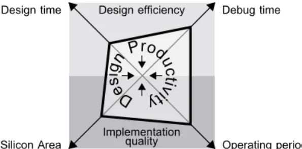
III. EVALUATING THEDESIGNPRODUCTIVITY OFHLS The performance of an HLS method is a trade-off between a system quality to optimize (frequency, area, memory...) and design efficiency. It can be illustrated by a radar chart such as the one in Figure 1. The smaller the polygon is, the higher the productivity because it means that both design efficiency and implementation quality are high. Note that period = 1/f requency is minimized to maximize frequency. Next sections introduce 3 metrics to assess an HLS method: the gain in NRE design time GN RE evaluating design
effi-ciency, the quality loss LQ evaluating implementation quality
and finally the design productivity PD evaluating the trade-off
between design quality and design efficiency. A. Evaluating Design Efficiency
Design efficiency results from a combination of many parameters including the complexity of the design under de-velopment, the amount of Non-Recurring Engineering (NRE) tasks to execute (i.e. the cost of the new code to produce),
Design time Debug time
Operating period Silicon Area Design efficiency Implementation quality De sign P rodu ctiv ity
Fig. 1. Example of a trade-off radar chart with implementation quality and design efficiency parameters.
the expressiveness, and “developer friendliness” of the design languages, the designer’s experience, the testability of the results, the simulation time (influencing the time of design and verification steps), and the maturity of the design tools.
Quantitative quality metrics can be computed to characterize the HLS and HDL codes. System development time can be divided into:
— 1.a NRE design time, i.e. time necessary for writing the code of a functionality,
— 1.b NRE verification time, i.e. time used for building a testbench and unit testing,
— 1.c the system integration time, i.e. time necessary to build from components a system respecting its requirements. The system integration time, comprising verification and validation, depends on features that go beyond digital system design (analog to digital conversion, energy management, physical environment, etc.). Reducing integration time by an HLS method would require a system completely defined with the HLS method, including for example I/O drivers. The system tested in this paper, like all systems using HLS today, integrates HLS generated blocks within a framework written with standard HDL. Integration time is thus considered out of the scope of this study.
Design times are controversial because they depend on the designer’s experience. Different times may be required for a design by a junior hardware designer and a senior hardware designer. In the experiments, design times measured for HDL and HLS reflect the time required by a single developer experienced on software signal processing but novice in both VHDL and CAPH languages. The experiments reflect the capacity of HLS to offer a high-level API to a novice designer. This choice is consistent with the important objective of HLS to open hardware design to a broader public of developers. A selection of the time taken into account in measurements reduces the subjectivity of the approach. The time taken to refer to books and papers for syntactic details is excluded from the measured time. The development times are thus sums of short design and verification times with a quantum of 1’ (minute) and an average length of 15’.
Code properties complement the timing results:
— 2.a number of Source Lines Of Code (SLOC) (excluding blank lines and comments),
— 2.b number of characters in the code (excluding blank lines and comments).
These grades reflect the complexity and expressiveness of the languages. A lower number of lines in the HLS code than in the HDL code reflects the abstraction of some implementa-tion concerns. These numbers do not fully reflest complexity, as for instance, one line of regular expression may have a greater complexity than 20 lines of C code. As a consequence, this information is not used in the DP metric but rather as an additional information.
B. Evaluating Implementation Quality
On an FPGA implementation, quality metrics are divided into area and time information:
— 3.a number of Look-Up Tables (LUTs) — 3.b number of registers,
— 3.c number of Random Access Memory (RAM) blocks, — 3.d number of Digital Signal Processor (DSP) cores. — 4.a processing latency,
— 4.b minimum operating period.
One number cannot reflect the capacity of an HLS method to improve a designer’s productivity. In order to make more objective the comparison between methods, a list of elements is displayed, providing a multi-dimensional evaluation of the Quality of Results (QoR). Even in this multi-objective context, giving a main DP metric to a method is necessary to compare different methods.
C. A New Metric of HLS Design Productivity
As HLS aims at reducing design time, the gain in global NRE time GN RE is the most important metric of design
efficiency. GN RE is defined formally as:
GN RE = tHDL design+ tHDLverif tHLS design+ tHLSverif (1) where tHDL
design and tHDLverif are respectively the design and
veri-fication times when writing the application in HDL. Similarly, tHLS
design and tHLSverif are the design and verification times when
writing the application in HLS. A time gain GN RE greater
than 1 reflects the ability of an HLS method to save design and/or verification time. If only design and verification times are evaluated to assess an HLS method, methods resulting in a fast design with low quality are favored. In the proposed method, a quality degradation metric is included that penalizes low quality systems.
Implementation quality metrics depend on the constraints of the design (strict frequency constraint, strong resource limitations...). To take into account in a single cost the different quality metrics constituting a QoR vector, the implementation cost is defined as the weighted sum of normalized features to minimize [15]. The normalization of the different hardware quality metrics is done with respect to the maximum amount on the chosen system. For instance, the maximum period of the design obtained with HDL is computed as:
prdHDLnorm= prd HDL
/prdsystemmax , (2)
where prdsystem
max is the maximum period for supporting the
application (for instance, to ensure the frame rate). In the general case of HLS DP measurement, we define quality loss as: LQ = P φHLS i ∈ΦHLSαi× (φ HLS i ) P φHDL i ∈ΦHDLαi× (φ HDL i ) , (3)
where ΦHLS is the sets of normalized quality metrics to
minimize and αi are normalizing coefficients. In particular,
in the case of an FPGA, we can define quality loss as:
LQ=
α1× lutHLSnorm+ α2× regnormHLS + α3× ramHLSnorm+
α1× lutHDLnorm+ α2× regnormHDL+ α3× ramHDLnorm+
α4× dspHLSnorm+ α5× latHLSnorm+ α6× prdHLSnorm
α4× dspHDLnorm+ α5× latHDLnorm+ α6× prdHDLnorm
(4) where lutHDL
norm and lutHLSnorm are numbers of LUTs (3.a),
regHDL
normand regHLSnormare numbers of registers (3.b), ramHDLnorm
and ramHLS
norm are numbers of RAM blocks (3.c), dspHDLnorm
and dspHLS
norm are numbers of DSP blocks (3.d), latHDLnorm and
latHLS
norm are latencies (4.a), and prdHDLnorm and prdHLSnorm are
operating periods (4.b).
The parameters αi can be tuned to favor different hardware
features. We propose 2 approaches: 1) architecture-relative where each alphai is set to 1, and 2) fair to place all metrics
on an equal footing, where each (non null) pair of values is normalized to its maximum:
αi= ( 0, if max(φHLSi , φHDLi ) = 0. (max(φHLS i , φHDLi ))−1, otherwise. (5) for φHLSi ∈ ΦHLS and φHDL i ∈ Φ HDL. The
architecture-relative approachis specific to a single device because it favors metrics that are sparse on the measured platform. Experimental results (Section VII) focus on the fair approach, putting all parameters on the same footing.
Quality loss LQ reflects the loss due to rising the level
of abstraction. A low LQ reflects a good HLS generated
code quality. We introduce the HLS Design Productivity (DP) metric as a unique grade to assess the trade-off between design efficiency and quality. HLS DP ratio is defined as:
PD= GN RE/LQ (6)
An HLS method can be considered successful if its DP is greater than 1. Two HLS methods can be compared in terms of DP, provided that the same approach is used for both methods, a greater DP reflecting a better trade-off between design efficiency and implementation quality.
D. Design Productivity Assessment Protocol
A few rules must be respected to evaluate in practice the DP of an HLS method versus HDL: the same hardware platform and the same synthesis (back-end) tools should be used for both HLS and HDL, the designer should have similar experi-ence in both the HLS and the HDL methods, the developed use case should have precise specifications and requirements, design periods in both languages should be interleaved, and the same (preferably default) synthesis tool configurations should be used for both HLS and HDL. A particular effort is made in this paper to obtain reliable DP measurements by following these different rules.
IV. EXPERIMENTALSET-UP TOMEASURE THEDESIGN
PRODUCTIVITY OF ANHLS COMPILER VERSUSHDL
In this section, details are given on the use case and the tools that this study leverages on to assess HLS vs. HDL. A. The HEVC Interpolation Filter Use Case
The motivations for using HEVC interpolation filtering as the application for design productivity assessment are three-fold. The use case is specifically chosen because it requires bit-exact implementation to conform to the HEVC standard. Moreover, it is based on canonical DSP operations. Finally, the HEVC interpolation filter requires only fixed point operations that are efficiently implementable on an FPGA.
Video compression leverages on redundancies between im-ages to reduce data rate. The performance of the latest video compression algorithms such as MPEG HEVC [8] is mostly due to a precise matching between blocks in an image and the corresponding blocks in near images. This matching must be precise also when a motion has occurred that is not an exact multiple of the pixel size. HEVC interpolation filters provide fractional-pixel motion compensation between images with a quarter-pixel precision on luminance.
The HEVC interpolation filter generates a shifted version of a block of pixels by applying a filter with coefficients (taps) generated from a Discrete Cosine Transform (DCT) and an Inverse Discrete Cosine Transform (IDCT) [8]. The block can be left shifted of 1/4, 1/2 or 3/4 of a pixel by the filter displayed in Figure 2. The upper part of the figure is a shift register. The filter coefficients tap[i] depend on the selected sub-pixel position σ. The filter has 8 taps for the 1/2 pixel position and 7 taps for the 1/4 and 3/4 positions [8].
x[t] tap[7] tap[6] x[t-1] tap[5] x[t-2] tap[4] x[t-3] tap[3] x[t-4] tap[2] x[t-5] tap[1] x[t-6] tap[0] x[t-7] y[t-7] 8 16 16 16 16 16 16 16 16 8 8 8 8 8 8 8 16 /64 10 clip8 8 horizontal filter input pixel flow
filtered pixel flow
Fig. 2. Signal flow of an HEVC interpolation filter for horizontal shift of 1/4, 1/2 or 3/4 of a pixel.
Figure 2 only represents horizontal filtering. The extension to a 2-D filtering version requires 8 horizontal filters. The re-sults of these filters undergo a second 8-tap filtering operation with equivalent coefficients for 1/4, 1/2 and 3/4 upper shifts. This bidirectional filter is illustrated in Figure 3 where line First In, First Out data queues (FIFOs) delay the pixels of one line length L to correctly synchronize the outputs of the different horizontal filters.
horizontal filter horizontal filter horizontal filter horizontal filter horizontal filter horizontal filter input pixel
flow picture line FIFO x[t] x[t-L] x[t-2L] x[t-3L] x[t-4L] x[t-5L] x[t-6L] x[t-7L] 8 16 16 16 16 16 16 horizontal filter horizontal filter 16 16 22 22 22 22 22 22 22 22 22 /642 10 clip8 8 filtered pixel flow y[t-7L-7] tap[0] tap[1] tap[2] tap[3] tap[4] tap[5] tap[6] tap[7]
Fig. 3. Signal flow of a 2-dimensional HEVC interpolation filter for horizontal and vertical shift of 1/4, 1/2 or 3/4 of a pixel.
The use case being normative, data sizing is derived from the standard specifications. This is an important point because it limits the design choices and helps comparing different versions of the code. The presented filters correspond to the core of the luminance filters. In the next sections, the presented filters serve as the basis for the HLS vs. HDL study.
B. Used Design Tools and Platform
The software tools and versions used for the study are:
• Altera Quartus II versions 13.1.0.162 and VHDL 2008,
• Mentor Graphics Modelsim ASE, delivered with Quartus,
• CAPH Compiler version 2.7.0.
A golden reference of the filter Design Under Test (DUT) is coded in C language. This implementation is out of the scope of the study and serves for verifying both the HDL and the CAPH implementations. The HDL code is ported to an FPGA-based smart camera named DreamCAM [16]. This camera embeds an Altera Cyclone III EP3C120F780C7N FPGA. Using a camera aims at making the study close to designer’s best practices by not limiting the study to simulations. A complex pattern of data valid signals makes the filter not trivial to port on the camera.
V. DESIGNINGHEVC INTERPOLATIONFILTERS INVHDL
In this section, the use case is implemented in HDL and qualitative as well as quantitative elements are given on the design effort. VHDL [17] is a language for hardware description standardized in 1987 and revised in 1993, 2000, 2002, and 2008. A VHDL program consists of explaining how a digital circuit is structured and what the behavior of each
component is. These behaviors can be purely combinatorial, sequential or more commonly mixed.
A. Writing the MPEG HEVC Interpolation Filters in VHDL 1) Assumptions and Verification of the Use Case Design: The number of possible designs in HDL for a filter such as the ones presented in Section IV is large. Accesses to external memory to store intermediate values can alter much the quality. It is also possible to use existing Semiconductor Intellectual Property Core (IP) blocks or “design templates” (especially for FIR filters). The choice of parallelizing or sequencing operations is also very important.
In order to narrow the design space, some assumptions are taken on the input and output pixel streams of our use case. The filter is synchronous to a unique clock and has asynchronous reset. The input pixel stream comes in raster order (i.e. scanning the image from left to right and from top to bottom) in a stream of 8-bit pixels. A data valid signal states whether the current clock event corresponds to a data value. Each filter configuration (1/4, 1/2 or 3/4 horizontal and vertical shifts) is studied independently and coefficients are considered constant. In an HEVC encoder or decoder, the filter must then be duplicated for the different positions. A sufficient number of clock events without data is given for the filter to resume execution at the end of a pixel line. The last assumption is compatible with most CMOS image sensors that provide horizontal and vertical blanking. The assumptions foster a pipelined design with FIFOs such as the ones illustrated in Figures 2 and 3. Several versions of the filter are designed with their test benches. The golden reference code in C language provides reference values for debug.
2) VHDL Version 1: Horizontal Filter with Minimal Inter-faces: In this version of the filter, implementing the diagram in Figure 2, the stream of input pixels is considered continuous (1 clock event = 1 data). A transition to zero of the data valid signal resets the filter. It is interpreted as the beginning of a new line and thus, the filter needs to gather 8 data before outputting the first valid data. Based on the writing of this HDL filter, the time needed to describe the pipelined quarter pixel filter in HDL is 358’ for design and 288’ for verification, including time for writing the test bench, RTL simulation, and debug.
The algorithm description time includes all the reflections on the description (data types, generics, sizing, the use of functions, data conversions, use of best practices...) and the writing, from scratch, of the VHDL files.
3) VHDL Version 2: Horizontal Filter with Interfaces for the DreamCAM Camera: When porting the filter onto the camera, the VHDL block must input and output a data valid signal (indicating pixel validity for each clock event) as well as a frame valid signal. The frame valid signal is continuously set during the reception of a frame and reset at the end of the frame. Clock events that do not carry data happen pseudo randomly during the reception of an image.
The time needed to describe the filter in HDL is 162’ for design and 783’ for debug, including 152’ on a test bench and
631’ on the DreamCAM platform. VHDL Version 2 shows that porting an algorithm onto a real platform has a large cost, even when the algorithm has already passed some RTL verification process.
4) VHDL Version 3: 2-D Filter with Interfaces for the DreamCAM Camera: This filter is designed by reusing the VHDL version 2 horizontal filter and combining filter results of several lines such as in Figure 3. The time needed to describe the filter in HDL is 232’ for design and 775’ for verification.
The main difficulties comes again from the control part of the filter that determines when a data is valid or not and on which cycle it must appear on a given signal. In particular, synchronizing data valid and frame valid signals have neces-sitated most of the time. Next section discusses the sources of VHDL non-optimality in terms of design productivity that make room for HLS methods.
B. Discussion on the Origins of VDHL Complexity
1) The Counterpart of VHDL Versatility: In order to build verifiable logic, it is recommended to design a fully syn-chronous system. Using VHDL, a designer is however free to design asynchronous circuits and gated clocks that are chal-lenging to verify. For instance, while rarely being necessary, latch constructs may be generated by mistake with VHDL, for instance with an incomplete IF T HEN ELSE statement in a combinatorial process. Latches are strongly discouraged in literature [17] and this type of “low level implementation bugs” is at the heart of the need for HLS methods [3].
2) A Unique Language for Different Objectives: A dif-ficulty of VHDL comes from the combination, in a single language, of simulation-oriented and implementation-oriented features. For example, operators such as modulus M OD or remainder REM are generally not synthesizable [17].
3) Some Unintuitive Properties: The absence of precedence in logical operators makes the following expression:
y <= a and b orc and d
equivalent to:
y <= ((a and b) or c) and d.
This property stands in contradiction to the mathematical order of operation and can cause errors that are difficult to detect for a new programmer.
4) The Historical Reasons: Some difficulties of the VHDL language come from the different techniques available to im-plement a single functionality. For instance, an 8-bit unsigned integer signal data can be declared by
SIGNAL data : INTEGER RANGE 0 TO 255;
or by
SIGNAL data : UNSIGNED (7 DOWNTO 0);
Choosing between the two solutions requires a knowledge that is not related to system design but rather to language implementation details. The integer style is typically used to manipulate data within a design while the unsigned style is used for designing I/Os.
5) The Fundamental Reason: The main productivity lim-itation while using VHDL is the tangle of value and timing concerns. A value is considered as correctly received only if it arrives at an exact predefined clock event. During design, a lot of time is spent to obtain a value one cycle later or, worse, one cycle sooner than what the current design outputs. As an input signal of an entity must be present when its corresponding valid signal occurs, much of the design time is spent to synchronize data and control signals.
Now that VHDL design characteristics have been presented, next section details for comparison the design of the same filter versions with the CAPH HLS language.
VI. DESIGNINGHEVC INTERPOLATIONFILTER INCAPH A. Introduction to the CAPH Language
CAPH [6] is a domain-specific language (DSL) for de-scribing and implementing stream processing applications on configurable hardware, such as FPGAs. CAPH was first released in 2011 and is based upon the dataflow model of computation where an application is described as a network of autonomous processing elements (actors) exchanging tokens through unidirectional channels (FIFOs).
As the CAPH language is not mainstream like the VHDL language, details on the syntax and semantics are given in this section. The behavior of individual actors in CAPH is specified using a set of transition rules, where a rule consists of a set of patterns, involving inputs and local variables, and a set of expressions, describing modifications of outputs and local variables. Tokens circulating on channels and manipulated by actors are either data tokens (carrying actual values, such as pixels for example) or control tokens (acting as structuring delimiters). With this approach, fine grain processing (down to the pixel level) is expressed without global control or synchronization.
Listing 1. An actor computing the sum of values along lists in CAPH.
actor suml in (i: signed<8> list) out (o: signed<16>) var st: {S0,S1}=S0 var s : signed<16> rules (st:S0, i:’<) -> (st:S1, s:0) | (st:S1, i:’v) -> (st:S1, s:s+v) | (st:S1, i:’>) -> (st:S0, o:s)
As an example, the actor coded in Listing 1 com-putes the sum of a list of values. Given the input stream < 1 2 3 > < 4 5 6 >, — where 1, 2, . . . represent data tokens and < and > control tokens respectively encoding the start and the end of a list — the CAPH program produces the values 6, 15. For this, the CAPH code uses two local variables : An accumulator s and a state variable st. st indicates whether the actor is actually processing a list or waiting for a new list to start. In the first state, the accumulator keeps track of the running sum. The first rule can be read as : when waiting for a list (st=S0) and reading the start of a new one (i=’<), then reset accumulator (s:=0) and start processing (st=S1). The second rule says : When
processing (st=S1) and reading a data value (i=’v), then update accumulator (s:=s+v). The last rule is fired at the end of the list (i=’>); the final value of the accumulator is written on output o. This style of description fits a stream-based execution model where pixels are processed “on the fly”.
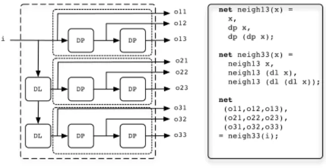
For describing the structure of dataflow graphs, CAPH embeds a textual Network Description Language (NDL). NDL is a higher-order, purely functional language in which dataflow graphs are described by defining and applying wiring func-tions. A wiring function is a function accepting and returning wires (graph edges). This concept is illustrated in Figure 4, where the dataflow graph on the left is described by the CAPH program on the right. In this example, two wiring functions are defined : neigh13 and neigh33. The former takes a wire and produces a bundle of three wires representing the 1 × 3 neighborhood of the input stream, by applying twice the one-pixel delay actor dp. The latter takes a wire and produces a bundle of nine wires representing the 3 × 3 neighborhood of the input stream, by applying the previously defined neigh13 function and the dl actor (one-line delay)
net neigh13(x) = x, dp x, dp (dp x); net neigh33(x) = neigh13 x, neigh13 (dl x), neigh13 (dl (dl x)); net (o11,o12,o13), (o21,o22,o23), (o31,o32,o33) = neigh33(i); DP DP DL DP DP DL DP DP i o11 o12 o13 o21 o22 o23 o31 o32 o33
Fig. 4. Example of a graph description in CAPH.
The tool chain supporting the CAPH language comprises a reference interpreter and a compiler producing both SystemC and synthetizable, platform-independent VHDL code. The SystemC back-end is used for verification.
B. Writing the MPEG HEVC Interpolation Filters in CAPH 1) Assumptions and Verification of the Use Case Design: The assumptions on the filter are the same as in the VHDL description case: pixel flow in raster order, unique clock, valid signal and sufficient blanking (Section V-A1).
Data validation is automated by the CAPH compiler based on the structural tokens < and > in the bitstream (Sec-tion VI-A). The CAPH environment provides FIFOs im-plemented in VHDL that automate data valid management. Moreover, a VHDL wrapper for the CAPH-generated VHDL code exists for the DreamCAM camera, driving inputs and FIFOs with the data valid signals of the camera. These features may appear unfair for the comparison between VHDL and CAPH but, in our opinion, VHDL and CAPH are treated on an equal footing, as they are both ported to the platform with tools helping the connection of their communication means
(signals in VHDL, FIFOs in CAPH) to their environment (a CMOS sensor and a USB port).
2) CAPH Version 1: Horizontal Filter with Minimal Inter-faces: In version 1 of the HEVC filter in CAPH, the code is composed of a single actor receiving the image bitstream and sending the horizontally filtered data. The test bench represents only 5 lines of code connecting the actor to the input and output streams. This simple test bench is possible because the HLS compiler performs only functional verification and time verification is left to the synthesizer. The actor implements a shift register and a counter discards the 7 first output tokens that do not represent valid data. The actor has four transition rules and most of the design time is taken to find the right way to represent the shift register in CAPH. In this version, the shift register is made of a set of internal variables in the CAPH actor. The filter is functionally equivalent to its VHDL counterpart after 103’ for design and 65’ for writing the test bench and debugging the filter with a SystemC simulation.
3) CAPH Version 2: Horizontal Filter with Interfaces for the DreamCAM Camera: Similarly to its VHDL counterpart, this version 2 of the filter in CAPH is adapted to the Dream-CAM needs, resetting the filter at the end of each line and adding modularity to the description. The filter is decomposed into 8 pipelined multiply-accumulate actors. The last actor in the pipeline has a different code. It gathers the intermediate products into a filtered and clipped value and generates the output flow. The main difficulty comes from getting rid of unwanted tokens, i.e. tokens that appear while the pipeline is filled up and emptied. The time for designing this version, composed of 9 actors, can be decomposed into 71’ for design and 72’ for verification.
4) CAPH Version 3: 2-D Filter: In this 2-D version of the filter, 7 new delay actors are first instantiated and connected. CAPH higher order functions are used to create a large number of actors with a code of limited size. Delay actors insert L first dummy tokens in the stream, where L is the length of a picture line, and then forward the arriving pixel values. The time needed to describe the 2-D filter in CAPH is split into 187’ for design and 169’ for verification.
C. Discussion on the Reduction of Complexity when using CAPH HLS Instead of VHDL
A dataflow Model of Computation (MoC) abstracts two elements:
• time. Instead of reacting to clock events, actors react to the arrival of data tokens,
• amount of data stored in FIFOs. The MoC assumes FIFOs of sufficient size to store pending tokens. These two abstractions make it possible a first verification of the process independently from the notion of time. The de-signer can thus verify very early in the design process whether the output values conform to the specification. Moreover, by generating SystemC code for simulation and verification, the CAPH compiler leverages on an optimized simulation environment. Writing the test bench in CAPH is also fairly less complex than in VHDL.
TABLE I
VHDLVS. CAPHDESIGN EFFICIENCY AND QUALITY FIGURES
(TIME IN MINUTES AND FREQUENCY INMHZ).
VHDL CAPH VHDL CAPH VHDL CAPH
v1 v1 v2 v2 v3 v3 N REdt 358 103 162 71 232 187 N REvt 288 65 783 72 775 169 # SLOCs 147 43 333 61 805 194 # chars 4114 1351 9465 2395 22072 6099 # LUTs 193 226 282 3161 2868 11398 (445) (3380) (11636) # Regs 81 103 115 2209 1252 7557 (269) (2375) (7723) # RAM 0 0 (1) 0 0 (1) 18 14 Freq. 64.7 68.0 71.8 83.0 65.2 84.2
These advantages come at the cost of a higher memory consumption, mostly due to the allocation of FIFO queues be-tween actors. Experimental results in the next section evaluate the DP of the CAPH HLS method w.r.t. VHDL by assessing both their resulting design quality and design efficiency.
VII. EXPERIMENTALRESULTS: EVALUATING THEDESIGN
PRODUCTIVITY OF THECAPH HLS COMPILER
A. Overview of the Experimental Results
Table I summarizes the experimental results of the different versions of the use case and Figure 5 illustrates them. Con-cerning CAPH results, values reported in brackets correspond to the total hardware resources including the overhead of the transformation from the platform signals (frame and data valid) to the token representation. These numbers are the fairest to compare to VHDL so they are the ones used for quality assessment.
Figure 5 displays values normalized to the largest of the two values. One can see that HLS is obtaining gains on design efficiency because, in the upper part of the charts, the CAPH values are smaller than the VHDL values (smaller is better). Conversely, there is a quality loss due to HLS that makes the VHDL values smaller than the CAPH values in the lower part of the chart. The CAPH HLS method is efficient for frequency; it even obtains slightly better minimum period than manual VHDL. This effect can be explained by the insulation of each actors by FIFOs that build a pipeline. However, CAPH presents a large overhead in terms of LUTs and registers. This effect is explained by the automatic insertion of FIFO queues between actors that are not present in VHDL (VHDL). Improving the footprint of the VHDL generated from CAPH is thus an important objective to make this HLS method competitive. Globally, a smaller area in the clear red zone than in the dark blue zone is a good indicator that HLS is reaching a higher DP than VHDL; this fact will be confirmed in the next sections.
B. Gain in NRE Design Time of CAPH vs. Manual VHDL Table II shows for each use case version the Gain in NRE Design Time GN RE introduced in Section III-C. In average,
NREdt NREvt SLOC LUTs Regs prd (a) v1 NREdt NREvt SLOC LUTs Regs prd (b) v2 NREdt NREvt SLOC RAM LUTs Regs prd (c) v3
Fig. 5. Design efficiency and implementation quality chart (the smaller the better) for each filter in CAPH (clear red) and VHDL (dark blue).
TABLE II
GAIN INNRE DESIGNTIMEGN RE, QUALITYLOSSLQANDDESIGN
PRODUCTIVITYPDOFCAPHVS.MANUALVHDL. CAPH vs. CAPH vs. CAPH vs. Average
VHDL v1 VHDL v2 VHDL v3
GN RE 3.84× 6.60× 2.82× 4.42×
LQ 1.70× 2.53× 1.47× 1.90×
PD 2.26× 2.61× 1.92× 2.26×
designing the use case versions with the CAPH HLS method took 4.42× less time than writing and testing VHDL by hand. The standard deviation is large (1.96). This fact shows that, depending on the code type (raw 1-D filter, 1-D filter with control or 2-D filter), the gain in design time varies.
C. Quality Loss of CAPH vs. Manual VHDL
The quality loss, defined in Section III-C, is evaluated to study the productivity of the HLS method. We focus in this paper on the fair approach, putting all parameters on equal footing to make results not very dependent on the type of FPGA so normalization to maximum values is skipped and parameters αi are computed by equation 5.
Numbers of DSPs and latency are ignored in quality loss computation (α4 = 0 and α5 = 0) because the use case
does not generate multipliers and the latency of a few cycles introduced by VHDL and CAPH is negligible when compared to the latency of several picture lines, mandatory in the 2-D filter, so latency does not reflect system quality.
Quality loss LQfigures are displayed in Table II. They show
that, when putting all quality metrics on an equal footing, there is in average a quality loss of about 2× due to using the CAPH HLS method when compared to VHDL manual writing. The standard deviation of 0.6 is limited.
D. Design Productivity of CAPH HLS versus Manual HDL From the previously computed gain in NRE design time and quality loss, we can derive the Design Productivity PD
for the different use case versions. The values of PDare shown
in Table II. The HLS Design Productivity (DP) metric for the tested CAPH compiler version 2.7.0 is 2.2×. This number is an evaluation of the gains obtained by the HLS compiler. The small standard deviation of 0.34 between the different versions is an encouraging sign of the relevance of the DP metric evaluation method proposed in this paper. Finally, one
can see in Figure I that while verification takes in average 3× the time of design in VHDL, it takes in average only 85% of the design time in CAPH.
VIII. CONCLUSION ANDPERSPECTIVES
In this paper, the notion of Design Productivity (DP) has been defined, as well as a method to assess the DP gains of an HLS method versus a manual HDL description. Using this method, an HLS compiler based on the CAPH dataflow programming language has been compared to manual VHDL. The framework for design productivity estimation pro-posed in this paper can be extended to any type of HLS and to any type of hardware systems. Figures of merit for the implementation quality and design efficiency should be adapted to the system under test. However, the method and recommendations remain valid. Crossbreeding different HLS methods and combining their best features in a unique method could drive the future of very-large-scale logic design.
ACKNOWLEDGMENT
This work has been partially supported by the HPeC ANR project.
REFERENCES
[1] “International technology roadmap for semiconductors - design,” 2011. [2] G. Martin and G. Smith, “High-level synthesis: Past, present, and future,”
IEEE Design & Test of Computers, no. 4, pp. 18–25, 2009.
[3] H. Ren, “A brief introduction on contemporary high-level synthesis,” in 2014 IEEE International Conference on IC Design & Technology, 2014. [4] E. Lee and T. M. Parks, “Dataflow process networks,” Proceedings of
the IEEE, vol. 83, no. 5, pp. 773–801, 1995.
[5] J. Eker and J. Janneck, “Cal language report: Specification of the cal actor language,” 2003.
[6] J. S´erot, F. Berry, and S. Ahmed, “CAPH: a language for implement-ing stream-processimplement-ing applications on FPGAs,” in Embedded Systems Design with FPGAs. Springer, 2013, pp. 201–224.
[7] Synflow, “The Cx programming language,” http://cx-lang.org, 2015, accessed: 2015-09-25.
[8] G. J. Sullivan, J.-R. Ohm, W.-J. Han, and T. Wiegand, “Overview of the high efficiency video coding (hevc) standard,” Circuits and Systems for Video Technology, IEEE Transactions on, vol. 22, no. 12, 2012. [9] T. Bollaert, “Catapult synthesis: a practical introduction to interactive c
synthesis,” in High-Level Synthesis. Springer, 2008, pp. 29–52. [10] J. Cong, B. Liu, S. Neuendorffer, J. Noguera, K. Vissers, and Z. Zhang,
“High-level synthesis for fpgas: From prototyping to deployment,” Computer-Aided Design of Integrated Circuits and Systems, IEEE Trans-actions on, vol. 30, no. 4, pp. 473–491, 2011.
[11] W. Meeus, K. Van Beeck, T. Goedem´e, J. Meel, and D. Stroobandt, “An overview of todays high-level synthesis tools,” Design Automation for Embedded Systems, vol. 16, no. 3, pp. 31–51, 2012.
[12] C. Lucarz, M. Mattavelli, M. Wipliez, G. Roquier, M. Raulet, J. W. Janneck, I. D. Miller, and D. B. Parlour, “Dataflow/actor-oriented language for the design of complex signal processing systems,” in DASIP Conference 2008, 2008, pp. 1–8.
[13] S. Ahmed, “Application of a dataflow programming language to the high level synthesis of real-time vision systems on reconfigurable hardware,” These de doctorat, U. Clermont, vol. 2, 2013.
[14] M. D. Zwagerman, “High level synthesis, a use case comparison with hardware description language,” Master Thesis, Grand Valley State University, 2015.
[15] O. Grodzevich and O. Romanko, “Normalization and other topics in multi-objective optimization,” in Proceedings of the Fields - MITACS Industrial Problems Workshop, 2006.
[16] M. Birem and F. Berry, “Dreamcam: A modular fpga-based smart camera architecture,” Journal of Systems Architecture, 2014.