Identification of urban surface materials using high-resolution hyperspectral aerial imagery

(1)

1

Université de Montréal

Par

Meghana Paranjape

Département de Géographie Faculté des Arts et des Sciences

Mémoire présenté en vue de l’obtention du grade de Maître ès sciences (M.Sc.) en géographie

Juillet 2019

(2)

2

Université de Montréal

Département de Géographie, Faculté des Arts et des Sciences

Ce mémoire intitulé:

Identification of urban surface materials using high-resolution hyperspectral aerial imagery

(Identification des matériaux de surface urbaine par imageries aériennes hyperspectrales à haute résolution)

Présenté par :

Meghana Paranjape

A été évalué par un jury composé des personnes suivantes

Liliana Perez Président-rapporteur François Cavayas Directeur de recherche Margaret Kalacska Membre du jury

(3)

3

Abstract

Knowledge of surface cover materials is crucial for urban planning and management. With advances in remote sensing, especially in high spatial and spectral resolution imagery, the identification and detailed mapping of surface materials in urban areas based on spectral signatures are now feasible. Spectral signatures describe the interactions between ground objects and solar radiation and are assumed unique for each type of material.

In this research, we use airborne CASI images with 1 m2 spatial resolution, with 96 contiguous bands in a spectral range between 367 nm and 1044 nm. These images covering the island of Montreal (Quebec, Canada), obtained in 2016, were analyzed to identify urban surface materials. The objectives of the project were first to find a correspondence between the physical and chemical characteristic of typical surface materials, present in the Montreal scenes, and the spectral signatures within the images. Second, to develop a sound methodology for identifying these surface materials in urban landscapes.

To reach these objectives, our method of analysis is based on a comparison of pixel spectral signatures to those contained in a reference spectral library that describe typical surface covering materials (inert materials and vegetation). Two metrics were used in order to measure the correspondence of pixel spectral signatures and reference spectral signature. The first metric considers the shape of a spectral signature and the second the difference of reflectance values between the observed and reference spectral signature. A fuzzy classifier using these two metrics is then applied to recognize the type of material on a pixel basis. Typical spectral signatures were extracted from two spectral libraries (ASTER and HYPERCUBE). Spectral signatures of typical objects in Montreal measured on the ground (ASD spectroradiometer) were also used as reference spectra. Three general types of surface materials (asphalt, concrete, and vegetation) were used to ease the comparison between classifications using these spectral libraries. The classification using ASTER as a reference library had the highest success rate reaching 92%, followed by the field spectra at 88%, and finally with HYPERCUBE at 80%. There were no significant differences in the classification results indicating that the methodology works independently of the source of reference spectral signatures.

(4)

4

Résumé

La connaissance des matériaux de surface est essentielle pour l’aménagement et la gestion des villes. Avec les avancées en télédétection, particulièrement en imagerie de haute résolution spatiale et spectrale, l’identification et la cartographie détaillée des matériaux de surface en milieu urbain sont maintenant envisageables. Les signatures spectrales décrivent les interactions entre les objets au sol et le rayonnement solaire, et elles sont supposées uniques pour chaque type de matériau de surface.

Dans ce projet de recherche nous avons utilisé des images hyperspectrales aériennes du capteur CASI, avec une résolution de 1 m2 et 96 bandes contigües entre 380nm et 1040nm. Ces images couvrant l’île de Montréal (QC, Canada), acquises en 2016, ont été analysées pour identifier les matériaux de surfaces.

Pour atteindre ces objectifs, notre méthode d’analyse est fondée sur la comparaison des signatures spectrales d’un pixel quelconque à celles des objets typiques contenues dans des bibliothèques spectrales (matériaux inertes et végétation). Pour mesurer la correspondance entre la signature spectrale d’un objet et la signature spectrale de référence nous avons utilisé deux métriques. La première métrique tient compte de la forme d’une signature spectrale et la seconde, de la différence des valeurs de réflectance entre la signature spectrale observée et celle de référence. Un classificateur flou utilisant ces deux métriques est alors appliqué afin de reconnaître le type de matériau de surface sur la base du pixel. Des signatures spectrales typiques ont été extraites des deux librairies spectrales (ASTER et HYPERCUBE). Des signatures spectrales des objets typiques à Montréal mesurées sur le terrain (spectroradiomètre ASD) ont été aussi utilisées comme références.

Trois grandes catégories de matériaux ont été identifiées dans les images pour faciliter la comparaison entre les classifications par source de références spectrales : l’asphalte, le béton et la végétation. La classification utilisant ASTER comme bibliothèque de référence a eu le plus grand taux de réussite avec 92%, suivi par ASD à 88% et finalement HYPERCUBE avec 80%. Nous

(5)

5

n’avons pas trouvé de différences significatives entre les trois résultats, ce qui indique que la classification est indépendante de la source des signatures spectrales de référence.

(6)

6

List of Tables

Table 2 Kappa coefficient and Variance of kappa coefficient of K-means classification with RGBI images ... 50 Table 3 Significance test using Z-score between K-means classification of RGBI images with

points under shadows and without points under shadows (NS- not significant) ... 51 Table 4 Confusion matrix using ASTER library as reference spectra with N=50 comparing three

classes, Asphalt, Concrete, and Vegetation ... 77 Table 5 Producer and user accuracy, omission and commission error of classification with

ASTER library ... 77 Table 6 Confusion matrix using HYPERCUBE library with N=50 comparing three classes:

Asphalt, Concrete, and Vegetation ... 78 Table 7 Producer and user accuracy, and omission and commission error for the classification

using HYPERCUBE library ... 78 Table 8 Confusion matrix using ASD library with N=50 comparing three classes: Asphalt,

Concrete, and Vegetation ... 79 Table 9 Producer and user accuracy, and omission and commission error of classification using

ASD library ... 80 Table 10 Pairwise z-score to assess the significant difference between classification based on

reference spectral signatures ... 80 Table 11 Spectral signatures remaining after classification of each reference spectral library .... 82

(9)

9

List of Figures

Figure 1 Graphical representation of sensors and their uses based on spatial, spectral, temporal,

and radiometric resolution (source: Kadhim, Mourshed, and Bray 2016) ... 17

Figure 2 Comparison of spatial resolution between two images of the same urban scene : A. an aerial imagery with 1m spatial resolution, and B. an aerial imagery with 25cm spatial resolution ... 18

Figure 3 The electromagnetic spectrum ... 20

Figure 4 Diagram of radiance (adpated from Bonn and Guy 1993) ... 20

Figure 5 Hyperspectral data cube (source: Shaw and Manolakis 2002) ... 21

Figure 6 Apparent spectral signature in radiance units multiplied by a factor of 1000 of pixel covered by vegetation extracted from an airborne CASI1500 image (1m spatial resolution) with 96 bands between 350 nm and 1100 nm ... 22

Figure 7 Schema of a mixed pixels and the linear combination of the spectral signatures it is composed of vegetation, background soil, minerals, and manmade materials (Source: Geo University, website: https://www.geo.university/courses/the-network-based-method-spectral-unmixing-framework)) ... 29

Figure 8 Interactions of photons causing a non-linearly mixed pixel (source: Dobigeon et al. 2014) ... 30

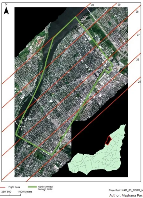
Figure 9 Study area with flight lines of CASI 1500 hyperspectral aerial imagery ... 34

Figure 10 The borough of Montreal North: mosaic of CASI 1500 hyperspectral imagery (true color composite bands 14 in blue, 28 in green, and 42 in red)) with the flight lines covering it ... 36

Figure 11 Flowchart of preliminary analysis to identify urban surface materials using linear spectral unmixing ... 37

Figure 12 Spectral signatures of asphalt and concrete (between 440nm and 2400nm) (source: Herold et al. 2004)) ... 39

Figure 13 Linear spectral unmixing results using hyperspectral CASI 1500 imagery of Montreal North (Montreal, Qc, Canada), bright shades represent higher proportions of vegetation, while dark shades represent lower portions of vegetation ... 40

Figure 14 Linear spectral unmixing results using hyperspectral CASI 1500 imagery of Montreal North (Montreal, Qc, Canada), bright shades represent higher proportions of asphalt, while dark shades represent lower portions of asphalt ... 41

Figure 15 Linear spectral unmixing results using hyperspectral CASI 1500 imagery of Montreal North (Montreal, Qc, Canada), bright shades represent higher proportions of concrete, while dark shades represent lower portions of concrete ... 42

Figure 16 Modal filter ... 43

Figure 17 Miss-positioning of validation points: two points said to be 'ready to plant' falling on an asphalt road ... 44

Figure 18 Concrete represented as bright pixels after linear spectral unmixing showing the potential for identifying urban surface materials ... 46

Figure 19 Differences in illuminations of two CASI images of the same scene taken on two separate days with different atmospheric conditions ... 46

(10)

10

Figure 20 Urban surface materials at potential planting points of a portion of Montreal North, Montreal, (QC) Canada ... 47 Figure 21 Urban surface materials of a portion of Montreal North using K-means clustering with

RGBI 20cm ortho-images ... 49 Figure 22 Flowchart of the fuzzy classification methodology used to identify urban surface

materials with hyperspectral data ... 53 Figure 23 Map of Montreal, Qc, Canada, showing the main land uses (source: Communauté

Métropolitaine de Montréal (CMM), website:

http://cmm.qc.ca/donnees-et-territoire/observatoire-grand-montreal/produits-cartographiques/cartes-pdf/ ) ... 55 Figure 24 Study area for fuzzy classification tile CASI_2016_08_20_103450h14v1 ... 56 Figure 25 Schema of flight line and field of view angle in the particular case of CASI 1500

hyperspectral imagery taken over the Island of Montreal (QC), Canada ... 60 Figure 26 Field of view from aerial imagery with CASI 1500 sensor in a Northward direction

and a Southward direction ... 61 Figure 27 List of spectral signatures from ASTER library used as reference spectra ... 63 Figure 28 Graphical representation of spectral signatures in the ASTER library (conifers in

green, construction concrete in blue, and black tar in black) ... 63 Figure 29 List of the spectral signatures from HYPERCUBE library used as reference spectra in

the fuzzy classification ... 64 Figure 30 Graphical representation of spectral signatures in the HYPERCUBE library (grass in

green, concrete in blue, and asphalt in black) ... 65 Figure 31 Graphical representation of spectral signatures in the ASD library (vegetation in green, concrete in blue, and asphalt in black) ... 66 Figure 32 List of spectral signatures from ASD library ... 67 Figure 33 Example of output image after running the shape similarity metric testing for a

reference spectral signature representing grass from ASD spectral library (light shades of grey indicate pixels that are more likely to resemble grass, while darker shades are less likely to resemble grass) ... 69 Figure 34 Description of the three possible zones in a fuzzy set A, where a is in the set, b is

outside the boundaries of the set, and c is in the fuzzy boundary of the set (source: Ross 2010) ... 71 Figure 35 Membership values (µ(x)) based on the boundaries of a set belonging to a fuzzy

classification (source: Ross 2010) ... 72 Figure 36 Schema of the fuzzy classification with set boundaries for the shape and the distance

criteria ... 73 Figure 37 Schema representing the combination of both shape and distance criterion for the

fuzzy classification ... 74 Figure 38 Comparison of spectral signatures representing Asphaltic concrete (taken from

ASTER spectral library), Concrete (taken from Hypercube spectral library), and Concrete medium (taken from the handheld ASD spectroradiometer spectral library) ... 84 Figure 39 Interpolation of reflectance values at CASI 1500 wavelengths with HYPERCUBE

spectral library ... 86 Figure 40 Distance similarity metric pitfall ... 88

(11)

11

List of Abbreviations

Abbreviation Meaning

ASTER Advanced Spaceborn Thermal Emission and Reflection Radiometer CASI Compact Airborne Spectrographic Imager

CMM Communauté Métropolitaine de Montréal DEM Digital Elevation Model

EM Electromagnetic

FWHM Full Width at Half Maximum HSS Hyperspectral Scanner System JHU John Hopkins University JPL Jet Propulsion Laboratory MLC Maximum Likelihood Classifier

MNF Minimum Noise Fraction Transformation MSAS Modified Spectral Angle Similarity

NIR Near Infrared

PCA Principal Component Analysis ROI Region of Interest

RF Random Forest

RGBI sensor Red, Blue, Green, Infrared sensor SAM Spectral Angle Mapper

SVM Support Vector Machine

USGS United States Geological Survey VNIR Visible and Near Infrared

(12)

12

Acknowledgement

I would like to thank my supervisor, François Cavayas, for guiding me through this research project. I would also like to thank my family, in particular my brother Kiran who helped me collect field data.

(13)

13

Chapter 1 - Introduction

1. Context and problem statement

1.1. Urban planning and management

With an increasing number of people living in cities, urban management and planning is important to insure a good quality of life in urban areas. According to a (United Nations, Department of Economic and Social Affairs, and Population Division 2014) urban populations reached 3.9 billion people worldwide. This number is projected to increase to 6 billion people by 2045. To accommodate the constant inflow of people towards cities, urban planners need adequate tools and data to properly plan and manage cities.

Many facets of urban life are considered to maintain or increase quality of life in a bustling city. Urban areas can be summarily defined as a landscape that is dominated by infrastructure where a large population exists, that works primarily in non-agricultural employment(Breckenkamp et al. 2015). These areas need to be organized to accommodate an ever-growing population; large infrastructure developments like residential areas, industrial area, and transportation; and linkages between infrastructure and the environment(Waddell 2002). Understanding the structure of urban like land use, or the material composition of the urban landscape, is important for many overarching urban planning and management agendas.

With climate change, global temperatures seem to increase, and urban areas are not exempt from this phenomenon. Temperatures are regulated in part by the types of materials found in cities. Often, in areas where there is little to no vegetation, temperatures are much higher than areas where vegetation exists. With an accurate cartography of urban surface materials, city planners can determine where temperatures are likely to be higher during heat waves and they can identify heat islands. Populations at risks of heat strokes can be warned to avoid these areas during heat waves. Once the heat islands have been identified, they can be the subject of temperature reduction efforts such as planting trees or demineralization.

(14)

14

Indeed, surface materials such as asphalt on roads, or, cement on sidewalks, or, even the grass and tree borders between roads and sidewalks, have a large influence on environmental factors in cities. This includes, among others, surface temperature, roughness and imperviousness. In turn, these will affect the quality of life of residents by regulating surface water flows, winds and air temperatures, air quality, and more intrinsic values of cities, like the aesthetic values of trees, health and social benefits of parks and natural areas(Tyrväinen et al. 2005).

The city of Montreal, Qc, Canada, is the second largest metropolitan area of Canada. It is the economic centre of the province and welcomes a large number of industries and professionals. It has been subject to flooding and increasing temperatures. Proper management of the city structure is vital to ensure a better quality of life to its residents. The City of Montreal does not have an accurate or up-to-date database of surface materials. Many of their projects require this database. For example, the mandate to green the city of Montreal by increasing canopy cover from 20% to 25% required them to know which planting sites needed to be demineralized. Most of their cartography identifies objects rather than materials, meaning that surface materials at planting sites was not available. There is a need for identifying surface materials in Montreal for better urban planning and management.

1.1. Problem statement

The composition of urban areas is a complicated and heterogeneous patchwork of different materials. Often, data on surface materials is acquired through fieldwork, which can be a tedious and time-consuming task. However, remote sensing can be a good alternative to this problem. It is the science of acquiring information at a distance on the Earth’s surface. Remote sensing exploits the interactions between objects and solar radiation. It can provide a faster and more affordable method for detecting ground objects such as trees in urban areas on a multi-annual basis (Myeong, Nowak, and Duggin 2006). Once a proper methodology for identifying surface materials has been established, monitoring over time will be much easier.

(15)

15

This research project aims to identify and map surface materials within an urban landscape to aid in city planning and management. More particularly, this study uses aerial hyperspectral images to identify surface materials, such as asphalt, cement, grass, and trees. Every ground object has in principle, a unique response to solar radiation that can be measured with hyperspectral imagery. This is a concept known as the spectral signatures.

The objectives of this study will therefore be:

1. Finding a correspondence between the type of surface cover material and its spectral signature within the images.

2. Developing a sound methodology to identify surface materials in urban landscapes, with high resolution hyperspectral aerial imagery.

The basic hypothesis for this study is that target objects have a unique spectral response measured with a hand-held hyperspectral sensor (spatial resolution of 1m and spectral range of 340-1050nm). It is then, possible to develop a methodology that can separate the objects based on this spectral response.

1.3. Thesis structure

This thesis is organized into six chapters. Chapter 2 is a literature review of the current research and methods within the field of hyperspectral imagery focused on identify surface materials. The third chapter explains some preliminary studies done in the context of a Research and Development project for the City of Montreal. The fourth chapter describes the main methodology used to identify urban surface materials with our images. It covers the study area and the methodology. We will also cover some preliminary analysis done earlier on in the project. Chapter 5, describes and discuss the results of our methodology for identifying urban surface materials. Finally, chapter 6, presents a general conclusion of the research project and suggests some improvements that could be the object of future research.

(16)

16

Chapter 2 - Urban remote sensing with

hyperspectral images: background

2.1. Sensors types and resolutions for urban remote sensing

Remote sensing has seen huge technological advances in imaging sensor types and image resolutions. Aerial photography was the most common imagery acquired when remote sensing first started being used. Cameras were mounted onto airplanes, and aerial photos were for reconnoitering purposes, especially during the First and Second World War (Borengasser, Hungate, and Watkins 2008). During the Cold War, the Arms Race helped encourage scientific discoveries such as the exploitation of the infrared part of the spectrum, and the development of observation technology like satellites, and sensors. A well-known example is the Landsat series of satellite that were developed by NASA, and were first launched into space in 1972, starting with Landsat 1. The objective of this series of satellite was, and still is, to observe Earth’s land masses and assess the quality of ecosystems, and the effects of land changes (Masek 2019). The last satellite of this series, the Landsat-8, has on board a multispectral sensor, which has spectral bands in the visible part of the spectrum as well as the near- and shortwave infrared, and a thermal infrared sensor. Over the years many satellites have been sent into orbits by different private and public organisms, equipped with wide range of sensors. Nonetheless, sensors have been consistently mounted on airplanes and other airborne technology such as drones.

Figure 1 illustrates the requirements in terms of spatial, temporal, radiometric, and spectral resolution of sensors in conjunction with different application fields. Examples of sensors, most of them onboard satellites, are also given.

(17)

17

Figure 1 Graphical representation of sensors and their uses based on spatial, spectral, temporal, and radiometric resolution (source: Kadhim, Mourshed, and Bray 2016)

Spatial resolution can be defined as the smallest discernible object in an image. It is also defined as the area of one pixel (also known as unit) representing the same area on the Earth’s surface (Campbell 2007). As urban areas are extremely heterogeneous environments, spatial resolution is an important factor to consider when choosing the type of remotely sensed data for projects. Imagery with high (metric) to very high (sub-metric) spatial resolution is required to properly identify and understand urban landscapes (Longley 2002). In present days, space borne sensors like those onboard of Digital Globe satellites, provide imagery with metric (in multispectral mode) and sub-metric resolution (in panchromatic mode). Airborne sensors providing very high spatial resolution are often used in various infrastructure and vegetation surveys in urban areas and risk

(18)

18

or emergency response modeling (Kadhim et al. 2016; Myint et al. 2011). Figure 2 shows two images of the same urban scene taken at metric and centimetric spatial resolution. It is clear that with a finer resolution (figure 2.B), it is easier to trace the boundaries of different objects and to identify objects like cars, or patterns on the street than with the larger resolution (Figure 4. A).

A B

Figure 2 Comparison of spatial resolution between two images of the same urban scene : A. an aerial imagery with 1m spatial resolution, and B. an aerial imagery with 25cm spatial resolution

Temporal resolution is the time lapse between each site visit. For satellites this is based on the orbital distances, while for aerial imagery, it depends on the time lapse between fly overs. Temporal resolution is a parameter to consider when performing urban growth and land cover change analysis which is not the case of our research project.

Radiometric resolution is the sensor’s ability to store detailed information on signal intensity in numeric format. In other words, it dictates the levels of grey that can be separated when translating the received signal from objects to numeric values. Modern airborne or space borne sensors provide images with 16 bits pixel depth (65536 levels of grey). Radiometric resolution determines the amount of information stored in each image, and the capacity (time and effort) needed to analyze the imagery. Images with a lower radiometric resolution will take much less time to analyze than images with a high radiometric resolution. The trade-off is of course, the quantity of data that can be acquired.

(19)

19

Spectral resolution is another parameter to consider while choosing data for an urban study. Spectral resolution is the capacity of sensors to register the incoming signal in small wavelength intervals. It can also be defined as the narrowest spectral interval that can be resolved by a sensor (Campbell 2007). The term hyperspectral imager (or imaging spectroradiometer) describes any imaging sensor operating in the optical part of the electromagnetic (EM) spectrum and acquiring data with high spectral resolution. Images are then composed of many dozens of narrow and contiguous spectral bands. Contrary to hyperspectral sensors, multispectral imaging sensors acquire images usually composed by no more than ten spectral bands. For instance, the airborne sensor used in the present research, the CASI 1500 (Compact Airborne Spectrographic Imager), can be programmed to acquire data with up to 288 spectral bands between 350 and 1050 nm compared to 8 bands of the multispectral sensor onboard the Worldview satellites operating approximately in the same spectral interval.

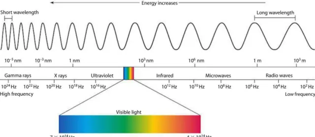
Modern technology allows the development of both multispectral and hyperspectral sensors operating within the well-known atmospheric windows of the near UV (350-400 nm), the visible (400nm-700nm), the near infrared (700-1100), the short wave (1100 -3000) and mid wave infrared (3000-5000) as well as the far infrared (thermal infrared: 8000-14000nm) (Figure 3). Although spectral resolution is deemed less important than spatial resolution in urban remote sensing, it still holds an important role in image analysis (Myint et al. 2011). High spectral resolution allows spectral analysis of the components of an image, which in turn can help identify various objects based on their spectral signatures (Myint et al. 2011). Our focus is on hyperspectral images in the interval from near UV to NIR (Near infrared) as used in the present research. The next section describes in more detail the processing and analysis methods of hyperspectral images for extracting information on surface material cover.

(20)

20

Figure 3 The electromagnetic spectrum

2.2. Hyperspectral imagery: processing and analysis

In the spectral interval of interest, hyperspectral images are created by capturing the solar energy reflected by a surface material and separating it into many spectral bands. The measured radiation per spectral band is expressed in radiance which is the radiant flux entering the sensor (Watt) per solid angle (steradian) of observation, per surface unit (m2) projected in the viewing direction of the sensor and per wavelength (µm) (Figure 4).

(21)

21

Hyperspectral data is often represented by a data cube (Figure 5). The x and y axis are the spatial axis, while the z axis represents the channels in which radiance measure are available (or the wavelengths the sensor was able to separate).

Figure 5 Hyperspectral data cube (source: Shaw and Manolakis 2002)

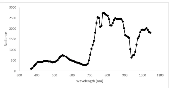
The apparent “spectral signature” (radiance values) per pixel shows clearly the potential of hyperspectral data to reconstruct the real spectral signature of a surface material (ground reflectance values) provided that atmospheric effects are corrected. In Figure 6, such an apparent spectral signature is drawn from our hyperspectral data set (see Chapter 3) with 96 bands. Radiation absorption effects of water vapour is evident in the NIR bands (band 50 and higher) with abrupt lowering of radiance values (hollows). The radiance values were provided to us with a multiplication factor of 1000. Conversion of measured radiance to ground reflectance is summarized in the next section.

(22)

22

Figure 6 Apparent spectral signature in radiance units multiplied by a factor of 1000 of pixel covered by vegetation extracted from an airborne CASI1500 image (1m spatial resolution) with 96 bands between 350 nm and 1050 nm

Various techniques are used to identify surface materials based on their spectral signatures. Most of the times these techniques are based on reference signatures found in spectral libraries or extracted from the images themselves (endmembers). Section 2.2.2 presents a review of these techniques.

2.2.1 Extraction of spectral signatures

Reflectance is an inherent optical property of a surface material and has values between zero and one as it is the proportion of reflected energy over the total amount of radiation incoming for the sun. Reflectance varies from one wavelength to another depending on the physicochemical structure of the surface material. Variation of reflectance throughout the solar spectrum is termed spectral signature, a way to signify that, theoretically, such variations are unique and depends solely on the surface material. Hyperspectral images are a high-density spectral sampling of EM energy more able to reconstruct the spectral signature of a surface material than a multispectral sensor. 0 500 1000 1500 2000 2500 3000 300 400 500 600 700 800 900 1000 1100 Ra di an ce Wavelength (nm)

(23)

23

However, the EM energy measured by a hyperspectral sensor is not directly related to the spectral signature of a material. As mentioned, the reflected solar energy measured by the sensor in a spectral band, is radiance (W/m2/sr/µm). Assuming a target reflects solar energy equally well in any direction (isotropic or Lambertian target), radiances vary not only with the reflectance of the examined targets but also depend on the atmospheric and solar illumination conditions during image acquisition. The incompatibility between radiance spectra and reflectance spectra is more important over urban areas where the atmosphere is usually loaded with gases and particulates (aerosol), which absorb and scatter solar radiation in various ways throughout the spectrum. As the particulates are usually concentrated in the troposphere, even in airborne imagery, as used in our study, atmospheric effects are almost always present. The airborne sensor has a wide field of view, atmospheric effects are not manifested in the same manner from one pixel to another. In our laboratory, we have access to a computer program ATMOCOR_CASI (in C-Sharp; François Cavayas personal communication) adapted to the particular acquisition conditions of our set of images provided by the airborne sensor CASI1500 (see Chapter 4 for more details). The program makes use of the various routines freely available of the 6SV atmospheric code (Vermote et al. 1997) written in FORTRAN to simulate gas absorption as well molecular (Rayleigh) and aerosol (Mie) scattering effects in both the incoming and the outgoing radiation path by considering (a) a particular atmosphere stratification with specific populations of gases and aerosol particulates per layer; (b) a particular composition of the aerosol loading (dust, black carbon, water soluble, salts), (c) the solar position and the sensor viewing conditions during image acquisition; (d) the type of surface reflection: isotropic or anisotropic; and (e) the altitude of the terrain as well as the height of the sensor (airborne case). By fixing the above-mentioned parameters the program converts the image radiances into ground reflectances in two steps.

The first step is to convert measured radiances into apparent reflectance factor (Equation 1). Reflectance factor is the ratio of the radiance measured by the sensor to the radiance of a perfect Lambertian target measured under the same viewing and illumination conditions as the target:

𝜌"#$"%& ∆𝜆, 𝜃", 𝜃+, 𝜑"− 𝜑+ =

𝜋 𝐿 ∆𝜆, 𝜃_", 𝜃₊, 𝜑_"− 𝜑₊ 𝐸₃ ∆𝜆

𝑑5 ∗ cos 𝜃"

(24)

24

Where 𝜌_"#$"%& is the reflectance at the sensor level at a spectral band ∆𝜆, L is the measured luminance at the same band, E0 is the solar radiance at the top of the atmosphere for an average

Earth-Sun distance (1 astronomical unit), cos 𝜃_" is the cosine of the sun zenithal angle 𝜃_", and d represents the distance between the Sun and the Earth at the moment of image acquisition (in astronomical units). In the above equation, all spectral quantities depend on the sun zenith angle (𝜃") and the sensor view zenith angle (𝜃+) as well as on the relative azimuth between the sun and the sensor (𝜑_" − 𝜑₊).

The second step is to correct apparent reflectance from atmospheric transmission and scattering effects. According to Vermote et al. (1997), under the assumptions of Lambertian target of infinite extent and a complete independence between atmospheric transmission and scattering, the apparent reflectance can be written as:

𝜌_"#$"%& ∆𝜆, 𝜃_", 𝜃₊, 𝜑_"− 𝜑₊ = 𝑇₌ 𝜃_", 𝜃₊ 𝜌_>?@ + 𝑇↓ _𝜃

" 𝑇↑ 𝜃+

𝜌_DE&=#D

1 − 𝑆𝜌_DE&=#D (2.)

For which, 𝑇=(𝜃", 𝜃+) is the transmission of gases (e.g. H2O, CO2, O2, and O3), 𝜌>?@ is the reflectance of the atmosphere due to Rayleigh and aerosol scattering, 𝑇↓ _𝜃

" represent incoming atmospheric transmission due to scattering (between the sun and the ground), and 𝑇↑ _𝜃

+ represent the reflected atmospheric transmission due to scattering (between the ground and the sensor); 𝜌_DE&=#D represents the ground reflectance factor for a Lambertian target. The expression

HIJKLMI

NOPHIJKLMI represents the radiation reflected by the infinite target after many interactions between

the target and the atmosphere with spherical albedo S. Radiation quantities depend on the position of the sun and the sensor viewing conditions. Chapter 4 presents in more details the way that the various parameters where fixed in the particular case of the images used in the present study.

(25)

25

In general, two main approaches are used to identify surface cover materials. The first one is an adaptation of classification algorithms developed for multispectral image analysis to the hyperspectral images. The second approach is based on the comparison of reference spectral signatures of the searched materials, usually extracted from external reflectance libraries, to the observed spectral signatures on the image. A third approach is also followed, usually with images of metric spatial resolution. In that case, reference spectra are used to establish the proportion of the surface of a pixel occupied by the reference materials (unmixing). These approaches are examined in the next paragraphs.

2.2.2.1 Classification algorithms

Many classification algorithms can be used to distinguish between surface cover materials on a pixel or a region (object) basis. Priya and Murugan (2013), present a general review of these algorithms. Usually the first step is to reduce the dimensionality of the hyperspectral data set given the redundancy in the information content of many spectral bands. Algorithms such as PCA (principal component analysis) or the MNF (minimum noise fraction transformation) are applied. Then training sites are selected and supervised algorithms are applied to the reduced image set. The study of Burai et al. (2015), in a complex rural environment, is a typical example of application of such algorithms with hyperspectral airborne images. The 128 original spectral bands in the 400-1000 nm (AISA sensor) were combined to create a dozen of bands with the MNF algorithm and used with three supervised classifications algorithms: the MLC (maximum likelihood), the SVM (support vector machine) and the RF (random forest) to identify 20 vegetation classes. All the algorithms were accurate enough (>80%) with 20 classes. The accuracy rises (> 95%) when the 20 classes are grouped to form 5 vegetation groups. While the SVM and RF algorithms can be applied with the original data set because their performance does not depend on the number of the training sites, the MLC is inapplicable in practice with the original data sets because, as the author demonstrate, his performance is heavily dependent on the number of training sites. With the image set of 128 spectral bands there is a need of at least 129 training sites.

The study of Chisense (2012), is another example of adapting the approaches used in the analysis of multispectral images to hyperspectral images. The author is interested on the identification of roof materials of buildings in a city in Germany. He uses the images of the airborne HyMap sensor

(26)

26

with 125 bands in the interval from 400 nm to 2500 nm (4 m of ground sampled distance). The building roofs are isolated using external data, an unsupervised classification algorithm (ISODATA) is then applied in order to extract training sites corresponding to 10 classes of roof material. After dimensionality reduction, the new image set is segmented into homogeneous areas and each area classified by a maximum likelihood object classifier. The obtained results are significantly accurate.

More sophisticated approaches are also proposed using variances of the C-fuzzy classification, neural networks, neuro-fuzzy networks, etc. (e.g. Kakhani and Mokhtarzade 2019). However even with such sophisticated approaches the number of identified surface materials (or land cover classes) are not significantly different from those identified with less sophisticated methods (and far less time-consuming approaches).

2.2.2.2 Use of reference spectral signatures

These approaches use similarity metrics between a reference spectral signature and an observed spectral signature on a pixel basis. The Spectral Angle Mapper, also known as SAM, is a classic example of this type of approach. The algorithm calculates the angle between the reference spectral signature and the image spectral signature. To accomplish this, spectral signatures are assumed to be vectors of n-dimensions (n-dimensions equal the number of bands within the image). The smaller the angle, the more similar the two spectral signatures are. A threshold value determines if their similarity is acceptable for a given class. Kruse et al. (1993), use the following formula (Equation 3) to describe the angle calculation:

𝛼 = cosON $USVN𝑡S𝑟S 𝑡_S5 $U

SVN $USVN𝑟S5

(3.)

where nb is the number of bands in the image, t is the image spectrum at pixel i, r is the reference spectrum, and α is the angle between the two spectra in radiance.

(27)

27

Certain authors prefer the use of the Modified Spectral Angle Similarity (MSAS) than simply the angle between the two spectra, as it has values between 0 and 2 (Homayouni and Roux 2004):

𝑀𝑆𝐴𝑆 =2𝛼 𝜋

(4.)

where MSAS is the modified spectral angle similarity, α is the angle between the reference spectrum and the image spectrum in radiance units.

Reference spectra can be found in spectral libraries such the NASA’s ASTER (Advanced Spaceborn Thermal Emission and Reflection Radiometer) library (Meerdink et al. 2019) or developed with in situ observations with handheld spectroradiometers. While existing spectral libraries are developed with laboratory measurements, in situ observations offer a better support as adapted to the materials present in a particular study area.

The use of SAM in urban areas has shown some success. As an example, Moreira and Galvão (2010) were interested in impervious surface materials identification in Sao Paulo, Brazil, with hyperspectral data. Their methods compared reference spectra from field surveys, done with a spectroradiometer, to pixel spectra from a hyperspectral aerial sensor, the airborne hyperspectral scanner system (HSS), with 2.7m spatial resolution and 37 spectral bands in the visible and near infrared portions of the EM spectrum. They found that overall accuracy of SAM classifier using all bands was 74%.

When using SAM for classification, a user defined threshold is used to classify image pixels based on their spectral angle between image spectrum and reference spectrum. The smaller the angle, the more likely the two spectra are similar. Mohammadi (2012) found that using a smaller threshold value made SAM classification more accurate. In his study that aimed to classify roads and assess their conditions, he used hyperspectral imagery, taken over Baden-Württemberg (Germany), to find asphalt, concrete, and gravel. A flaw he found with SAM, was the large number of unclassified pixels. With a low threshold value, many calculated angles between reference and pixel were too large to be classified in an appropriate class; resulting in many unclassified pixels.

(28)

28

Other studies show different accuracy levels for SAM classifiers. A study in China that used aerial hyperspectral and satellite hyperspectral imagery to identify hazardous surface materials had an 86% success rate, compared to only a 65% success rate using different spectral image classifier (Ye et al. 2017). The authors also found that the optimal threshold angle changed depending on the type of material that needed to be identified. For example, recognizing steel rooftops with SAM was best accomplished with a threshold angle of 0.25 radians, while identifying roads made of asphalt was easier when using threshold of 0.1 radians. Overall, the study found that SAM had potential for material identification in urban areas. However, a study that aimed to identify tree species in a forested area with hyperspectral imagery of 1m resolution only found that SAM had an overall accuracy of 48.83%. Other classifiers used in the study had a much better accuracy level, going up to 85.56% when using MLC (Shafri, Suhaili, and Mansor 2007). One of the differences between these two studies is the area of study. One study looks at an urban area with many types of materials with spectral signatures that have different shapes, while the other tried to differentiate between tree species that have more or less the same shape. The SAM algorithm was not well suited for differentiating between spectral signatures that had the same shape such as tropical tree species.

2.2.2.3 Unmixing

As remotely sensed urban scenes are characterized by heterogeneous materials in close proximity and or adjacent to one another, often pixels found within the image are considered mixed. That is to say mixed pixels are pixel that hold more than one material in varying proportions. There are two common reasons for mixed pixels to occur, the first is that spatial resolution of an image. If the spatial resolution is too low, multiple objects can be represented in one pixel. For example, if a pixel of 5m is at the border between a sidewalk and a garden, then the pixel will have spectral signatures of both grass, and cement. The second reason mixed pixels occur is when the nature of the material itself is mixed. For example, a pixel representing a piece of road is composed of all the materials that go into making an asphalt road which are asphalt, cement, rocks, etc. (Keshava and Mustard 2002).

(29)

29

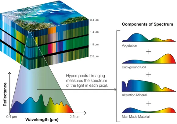
In order to deal with mixed pixels, spectral unmixing algorithms were developed. In hyperspectral data, the high spectral resolution allows the identification of different spectra representing the varied materials in each mixed pixel (also known as mixels). Figure 7 illustrates this idea with a hyperspectral data cube. In fact, the pixel’s spectral signature can be thought of as a weighed combination of unique spectral signatures of materials present on the ground at the location of said pixel. The combination is simplified to a linear relationship mathematically represented by equation 5:

Figure 7 Schema of a mixed pixels and the linear combination of the spectral signatures it is composed of vegetation, background soil, minerals, and manmade materials (Source: Geo University, website: https://www.geo.university/courses/the-network-based-method-spectral-unmixing-framework))

ρ[λ]=s1ρ1[λ] + s2ρ2[λ] + ⋯ + snρn [λ] (5.)

with ρ[λ] the reflectance of a pixel at wavelength λ, sn the proportion of each distinct object with reflectance ρn.

(30)

30

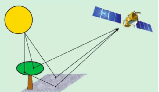
Linear unmixing models suppose that each radiative interaction is unique by the time it has reached the sensor. This assumption is often criticized as photons tends to interact with many objects and bounce off a multitude of materials. To account for these multiple interactions, nonlinear models were created. However, when considering non-linear unmixing, it is very difficult to model multiple light interactions, as the properties change with the smallest disruption to the light’s initial path (Dobigeon et al. 2014). Figure 8 shows bidirectional interactions of photons with the surface of the Earth, one of the many possible non-linear interactions. Equation 6 describes nonlinear models (Plaza et al. 2007),

𝑟 = 𝑓(𝐸, 𝛼) + 𝑛 (6.)

where 𝑓(𝐸, 𝛼) represents a nonlinear function describing the relationship between E and 𝛼, and 𝑛 represents the correction factor for noise in the image.

Figure 8 Interactions of photons causing a non-linearly mixed pixel (source: Dobigeon et al. 2014)

Heiden et al. (2001) have done many studies to classify urban surface material in Dresden, Germany. They use the airborne sensor HyMap data, with 6m resolution and 128 spectral bands ranging from the visible to the shortwave infrared. As noted earlier most urban remote sensing studies are accomplished with sub-metric spatial resolution, however, this is only in more recent

(31)

31

studies as the technology has improved. In the early 2000’s most studies were done with resolutions under 10m. Heiden et al. (2001) study aimed to create a detailed spectral library of urban materials based on a predetermined subdivision by infrastructure types. The second objective of the study was to identify surface materials based on their spectral characteristics. In order to do this, they performed spectral unmixing techniques to account for mixed pixels. Their method was very successful and reached 99.8% classification of the area, more than half of which was composed of mixed pixels. As each spectral signature has a unique shape and can be identified by its discrete absorption features, Heiden et al. (2001), ascertain that a robust spectral library can greatly improve the ability to successfully classify urban areas.

Some studies have found that using a combination of different classifiers helps increase accuracy levels. Indeed, Segl et al. (2003) found that finding image feature based on shape (or shaped base feature identification algorithms), helped differentiate between objects commonly found in urban areas such as buildings, open areas, etc. Once there “shapes” were found, seedling pixels could be assigned more precisely. Seedling pixels are pixels that are spectrally pure, similar to the endmember concept. Once seedling pixels were identified, an unmixing algorithm was performed on the urban study area. They compared the success rate for identifying surface materials using only spectral unmixing and shape. They found that using a combined methodology helped to better differentiate between materials and increased accuracy.

2.3 Partial conclusions

Identifying surface cover materials in urban areas using hyperspectral imagery is a challenging operation. Until today there is not a clear indication in the way to attack this problem. Our data set is composed by images of one meter spatial resolution (see next chapter). So, mixed pixels should be present and linear unmixing approach is a simple and interesting way to address the material identification problem. The other approach we decided to follow is to develop similarity metrics between reference and observed spectral signatures such as the shape metric and an approach to decide to the degree of similarity which is independent of thresholds.

(32)

32

Chapter 3 - Preliminary studies

This chapter is an overview of the preliminary analysis performed to identify urban surface materials. In the context of a Research and Development project with the City of Montreal, we performed a series of preliminary analysis on our CASI images. The goal of the project was to develop a methodology to identify urban surface materials to aid with planting efforts in Montreal. The City of Montreal had a mandate to green the city by increasing the greenness index from 20% to 25%. In order to accomplish this goal, they wanted to plant trees on public property throughout the city. However, removing asphalt, concrete, or other building materials can incur an enormous cost. Therefore, they needed to know the scope of this greening project by having a detailed database on urban surface materials in Montreal. They could have acquired this information with field surveys but to cover the entire island would have demanded a large mobilisation of personnel and resources. Remote sensing of urban materials offered them an alternative to field surveys.

The city completed a theoretical exercise in which geomatics professionals created a sample of 1265 geo-located points where trees could potentially be planted on public property (e.g. sidewalks) free of any structure (e.g. lamps, bus stops). They needed a way to find out if these potential locations were in a state to be immediately be planted in (e.g. bare soil or grass cover), or if site preparation was needed before planting (e.g. cement or asphalt removal). In the last case, this would incur larger costs, and more time for the plantation efforts.

The city of Montreal also provided us with field points for which surface materials had been identified. These points were geo-located and solely situated on public property. They were used as validation points for the methodology.

This chapter is divided into two sections. The first section describes the methodology to identify urban surface materials using the CASI 1500 images. While the second section describes some tests made with the multispectral high-resolution aerial imagery taken with a VEXCEL- VNIR

(33)

33

(visible and near infrared) camera. This second section permits us to assess the potential of using sub-metric imagery for urban studies as opposed to the metric CASI 1500 imagery.

3.1. CASI imagery analysis

Our experiment was based on airborne hyperspectral imagery acquired by the City of Montreal in the summer 2016 covering the entire Montreal Island. The sensor was CASI 1500 operated by the company ITRES (Calgary, Canada). Figure 9 shows the flight lines followed over the city to obtain the images. These were separated into two zones, the first where the flight lines overlapped by 50%, the second where the flight lines overlapped by 35%. The flight line overlap changes to account for changing topography and tall buildings. The altitude of the flight lines varies between 887 m and 914.8 m. Due to adverse atmospheric conditions, the coverage of the whole Island spread at different times in August and early September and were acquired between 13:00 and 16:00. The frame time was fixed to 18ms. The images had a 1m spatial resolution and a spectral resolution of 96 contiguous bands spanning between 380 nm and 1040nm with a bandwidth of 7.2 nm. That is to say, the images cover the visible portion of the EM spectrum as well as most of the NIR, with band intervals approximately 5 nm in width.

(34)

34

(35)

35

The study area for these preliminary analyses was the borough of Montreal North (Figure 10). This borough has a very heterogeneous landscape and lacks a lot of greenery. That is why city officials thought it would be a good place to issue a priority planting mandate. Montreal North is an area with large industrial zones composed of building materials such asphalt and cement. Most of these industrial zones have large parking lots associated with them, which increases the built portion of the borough. Residential areas cover a large area of the borough and clearly have more greenery than commercial or industrial zones. The following figure shows an overview of Montreal North, with flight lines that went through it. One can also see, that the CASI imagery shows many grey buildings (built materials), and little or sparse greenery (or vegetation).

(36)

36

Figure 10 The borough of Montreal North: mosaic of CASI 1500 hyperspectral imagery (true color composite bands 14 in blue, 28 in green, and 42 in red)) with the flight lines covering it

As the images cover an urban area with 1m spatial resolution, pixels often covered an area with many materials, and would be considered mixed pixels. Therefore, we decided that linear spectral unmixing would be suitable for this initial analysis. As explained in equation 5, linear spectral unmixing supposes that a pixel’s spectral signature is the weighted combination of spectral

(37)

37

signatures of the materials that can be found within that pixel. To ease computational needs of the study we limited our tests to public property.

3.1.1. Methodology of preliminary study with CASI 1500 imagery

Figure 11 is a flowchart of the preliminary methodology used to identify urban surface materials with the CASI 1500 images. The first step of the methodology was to convert our images from radiance to reflectance. Then, we needed to find our regions of interest which were used as the reference spectra to run the linear spectral unmixing algorithms. Finally, these unmixing results were classified to obtain a final cartography of surface materials in Montreal North. This classification was validated with the geo-located points provided by the City of Montreal. These steps are described in more detail in the next paragraphs.

(38)

38

The aerial images were provided to us in radiance units. We converted the radiances into apparent reflectance using the flight parameters, the position of the sun during acquisition, as well as the spectral solar radiation. Equation 1 describes the conversion formula (see Chapter 2). Usually, after this first conversion, we would need to perform atmospheric corrections to obtain object ground reflectance. However, at this stage in our study we had not created the atmospheric corrections algorithm used in the rest of the study (see Chapter 4). Therefore, we proceeded with apparent reflectance for the spectral unmixing algorithms.

3.1.2. Spectral unmixing

3.1.2.1. Reference spectral signature

The City of Montreal wanted us to identify were asphalt, concrete, cobblestone, low vegetation, and other inert materials. Spectral signatures for these materials can be found in spectral libraries measured with in situ methodologies using spectroradiometers. However, because the images were not yet atmospherically corrected, it was not possible to use spectral libraries as reference spectra. Instead, we used pixels within the image that contained only one material. These pixels are ‘pure’ pixels and are used as ‘endmembers’ and are input as reference spectra in our study.

We found these pure pixels using the region of interest (ROI) method. ROIs provide an average spectral signature for every material of interest. They are contiguous groups of pixels throughout the image grouped into polygon representing one type of material. By taking ROI’s throughout the image, we can take into consideration some illumination variation. We can also take into consideration the variability of the spectral signature of the same type of material. Figure 12 gives an example of the spectral signatures possible of asphalt and concrete.

(39)

39

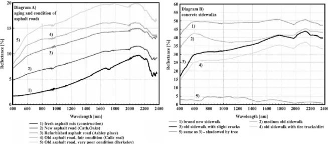
Figure 12 Spectral signatures of asphalt and concrete (between 440nm and 2400nm) (source: Herold et al. 2004)) 3.1.2.2. Unmixing and Classification

These average spectral signatures were used to run a linear spectral unmixng algorithms. The results we obtained were one new image for each type of material we had chosen to separate. For each pixel, we had the proportion of the material that could be found in it. Some examples are shown in figures 13 to 15.

(40)

40

Figure 13 Linear spectral unmixing results using hyperspectral CASI 1500 imagery of Montreal North (Montreal, Qc, Canada), bright shades represent higher proportions of vegetation, while dark shades represent lower portions of vegetation

(41)

41

Figure 14 Linear spectral unmixing results using hyperspectral CASI 1500 imagery of Montreal North (Montreal, Qc, Canada), bright shades represent higher proportions of asphalt, while dark shades represent lower portions of asphalt

(42)

42

Figure 15 Linear spectral unmixing results using hyperspectral CASI 1500 imagery of Montreal North (Montreal, Qc, Canada), bright shades represent higher proportions of concrete, while dark shades represent lower portions of concrete

Finally, we had to classify the results of our spectral unmixing. For this we used a binary decision tree to create 46 classes based on the variability statistics of each image after unmixing. The 46 classes gave us an idea of the proportion of target materials in pixels. In order to simplify validation efforts, we grouped these 46 classes into 4 overarching classes by visual interpretation of the images. The four classes were asphalt, concrete, vegetation, and other. If the pixel had equal to low proportion of one or many materials than it was classified into the category it appeared to be by photo-interpretation. We also created a much simpler classification that classified the pixels by the material that had the largest proportion in each pixel. This lead to an end classification with 4 classes: asphalt, concrete, vegetation, and other. This second classification was not subject to photo-interpretation errors. It simply took the material that had the largest proportion in each pixel as the final classification.

(43)

43

3.1.3. Results and discussion

We validated the classification using the potential planting points for which the ground surface materials were known. A sample of 185 points were used that covered the study area. For both types of classification, the results were less than optimal, reaching overall success rates of 49% and 55%. In light of these poor results, we tried to find sources of errors.

First, we decided to reclassify the pixels with a modal filter with a window of 3 x 3. With this filter, the central pixel would take the most prolific value of the 9 pixels in the 3x3 window. An example is given in figure 16: the central pixel has a value of 1 and would be transformed into a value of 2 by the modal filter, as the value of 2 is the most common value in the 3x3 window. The results of the classifications were slightly better but still low, reaching overall success rates of less than 60%. About 40% of the total number of pixels that fell under the 1265 theoretical planting points for which surface materials were known, changed values after the filter was used. This indicates that the points fall in areas of transition for which dominant material identification is less certain.

Before modal filter After modal filter

Figure 16 Modal filter

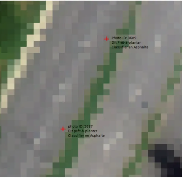
Another source of error could have been the fact that certain points did not correctly fall in their geographic positioning (Figure 17). This may be due to the inherent error in orthorectification of the hyperspectral images. It may also be due to the error associated with point’s acquisition

(44)

44

method. Indeed, the points were taken with satellite and GPS technology in differential mode with the WAAS correction system. The error in geolocation is between 0.50m and 1m for 1 standard deviation. If we were to take a confidence interval of 95%, (𝛔=1.96), then the positioning error would increase to ± 3.3m. A clear example of this error is illustrated in the following image (figure 18) for which the pixels under the points were classified as asphalt, which seems correct by photo-interpretation. However, field inventory of these points was said to be ‘ready to plant’, meaning they should have been located on the grass about three pixels to the right of their current location.

Figure 17 Miss-positioning of validation points: two points said to be 'ready to plant' falling on an asphalt road

The last source of error we thought could have affected the results was shadowed areas. When pixels fall under shadowed areas from buildings or canopy, it is much harder to obtain a spectral

(45)

45

response from them. This low spectral response could have led to errors during classification. We decided to tests if excluding shadowed areas would increase classification results. Shadowed areas were identified using a 1m DEM (Digital Elevation Model), acquisition meta data, and the ArcGIS tool ‘Area Solar Radiation’. We masked all the shadowed areas, and excluded the potential planting points that fell in these areas. However, we did not manage to increase the classification results. It does not seem that shadowed areas affect the results, especially since only 4% of the total number of potential planting points fall under shadowed areas.

3.1.4. Conclusion

Spectral unmixing has some potential for identifying the dominant materials of pixels. Looking more closely at certain unmixing images, it is clear that a distinction of certain material was made. Indeed, figure 18, the concrete sidewalks are apparent and much brighter than any surrounding area. Visually, it would appear that the unmixing algorithm did indeed manage to separate concrete. Perhaps, the decision tree classification was not best suited for the final classification. Also, the lack of atmospheric corrections may have created some confusion during classification. Figure 19 shows imagery of the same scene on two different acquisition dates. The illumination is different and depends partially on atmospheric conditions. The low success rates of the classification presented in these preliminary studies lead us to pursue a new methodology.

(46)

46

Figure 18 Concrete represented as bright pixels after linear spectral unmixing showing the potential for identifying urban surface materials

Image taken on 23/08/2016: Sun at 56° over the horizon and looking almost completely South

Image taken on 2/09/2016: Sun at 45° over the horizon and looking South-East

Figure 19 Differences in illuminations of two CASI images of the same scene taken on two separate days with different atmospheric conditions

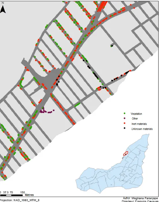
Images with a metric resolution provide a general understanding of urban surface materials and can be used as a preliminary dataset to assess the costs and optimal locations of planting. Figure 20 is an example of the type of cartography achieved with this method. Due to the large

confusion between asphalt and concrete we grouped these two classes into one category named inert materials. Also, since this particular scene was taken with an overlap of two flight lines, any point in these overlap that did not have the same classification on both occasions was reclassified as ‘unknown materials’. For example, if a point on one flight line was classified as vegetation, but the same point on a different flight line was classified as asphalt, then it was deemed ‘unknown material’.

(47)

47

Figure 20 Urban surface materials at potential planting points of a portion of Montreal North, Montreal, (QC) Canada

3.2. Multispectral imagery RGBI

(48)

48

The tests performed with the RGBI (Red, Green, Blue, Infrared) imagery were only performed on one tile (#0011). This tile covers an area of approximately 1.6km x 1.6km with a 20cm ground resolution. The tile was classified with a K-means algorithm. This algorithm is an unsupervised classification that separates the spectral space along n-axes in our case: red, green, blue, and infrared. The number of clusters (K) is defined by the user and will represent the number of classes at the output. The algorithm uses the digital numbers of a sample set of pixels (also user defined). By iterative process, the algorithm finds the centre of gravity of the K

clusters. Then each pixel is classified into a cluster in a way that minimizes the spectral distance E between the centre of gravity of the cluster and the pixel value (equation 7) (PCI Geomatics 2017). The results are the K-clusters that need to be assigned to a specific class.

𝐸 = 𝑥 − 𝑚_S 5

a∈cd

e

SVN

(7.)

In this equation, x is a spectral representation in space of the object, 𝑚_S is the mean of cluster 𝐶_S.

For the purpose of this test we limited the processing to the public areas of the tile. This reduced the overall computation requirements of the algorithm.

3.2.2. Results and validation

We ran the algorithm to produce 16 groups of pixels. These groups were reclassified into 7 classes by photo-interpretation as follows: 0- unknown, 1- shadows, 2- trees and high vegetation, 3- low vegetation, 4- asphalt, 5- concrete, and 6 – very bright objects. Figure 21 shows the results of the classification after photo-interpretation over a portion of the Montreal North.

(49)

49

Figure 21 Urban surface materials of a portion of Montreal North using K-means clustering with RGBI 20cm ortho-images