Reader Design for Chipless Millimeter-Wave Identification (MMID)TAG
77
0
0
Texte intégral
Figure
![Figure 1.1. A RFID system [4].](https://thumb-eu.123doks.com/thumbv2/123doknet/2352907.36664/17.918.111.770.555.793/figure-a-rfid-system.webp)
![Figure 2.1. Structure and operation of a typical chipless tag encoded in the frequency domain [3]](https://thumb-eu.123doks.com/thumbv2/123doknet/2352907.36664/20.918.168.746.221.484/figure-structure-operation-typical-chipless-encoded-frequency-domain.webp)
![Figure 2.3. Typical encoded signal of frequency domain based chipless tag [3].](https://thumb-eu.123doks.com/thumbv2/123doknet/2352907.36664/21.918.189.730.389.657/figure-typical-encoded-signal-frequency-domain-based-chipless.webp)
![Figure 2.7. Widely used circuit symbols of coupler [3].](https://thumb-eu.123doks.com/thumbv2/123doknet/2352907.36664/24.918.209.675.105.362/figure-widely-used-circuit-symbols-coupler.webp)
+7
![Figure 2.16. Intermodulation products [10].](https://thumb-eu.123doks.com/thumbv2/123doknet/2352907.36664/31.918.259.657.108.335/figure-intermodulation-products.webp)
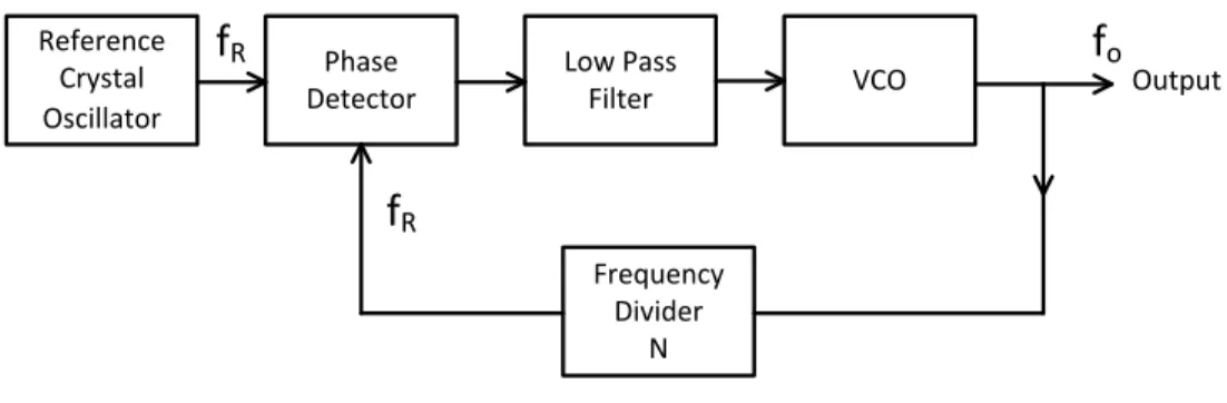
![Figure 2.21. Generation of a wideband frequency signal using a VCO [3].](https://thumb-eu.123doks.com/thumbv2/123doknet/2352907.36664/33.918.223.709.684.870/figure-generation-wideband-frequency-signal-using-vco.webp)
Documents relatifs
In this paper, an on-chip dual-band rectangular slot antenna, is proposed and demonstrated for a new generation of high data-rate, battery-free, yet active millimeter-wave
