A Time-Domain Vibration Observer and Controller for Physical
Human-Robot Interaction
This paper is a Post-Print version (ie final draft post-refereeing). For access to Publishers version, please access http://www.sciencedirect.com/science/article/pii/S0957415816300277.
Elsevier 2016.
Alexandre Lecoursa,∗, Martin Otisb, Pierre-Luc Belzilea, Cl´ement Gosselina
aD´epartement de g´enie m´ecanique, Universit´e Laval, Qu´ebec, Canada, 1065 Avenue de la M´edecine, G1V 0A6 bD´epartement des sciences appliqu´ees, Universit´e du Qu´ebec `a Chicoutimi, Saguenay, Qu´ebec, Canada
Abstract
This paper presents a time-domain vibration observer and controller for physical Human-Robot Interaction (pHRI). The proposed observer/controller aims at reducing or eliminating vibrations that may occur in stiff interactions. The vibration observer algorithm first detects minima and maxima of a given signal with robustness in regards to noise. Based on these extrema, a vibration index is computed and then used by an adaptive controller to adjust the control gains in order to reduce vibrations. The controller is activated only when the amplitude of the vibrations exceeds a given threshold and thus it does not influence the performance in normal operation. Also, the observer does not require a model and can analyze a wide time frame with only a few computations. Finally, the algorithm is implemented on two different prototypes that use an admittance controller.
Keywords: Physical Human-Robot Interaction, Vibration reduction, Admittance control, Intelligent assist device, Vibration control, Robotics
1. Introduction
Although robots have been used for several decades, direct physical interactions between robots and humans are rare, for obvious safety reasons. The most evident means of ensuring safety is to
5
segregate robots and human beings thereby leading to robots designed and programmed to work in a closed cell. However, in several applications, it is desirable to exploit the force capabilities of robots by directly combining them with the skills of a
hu-10
man being, hence leading to human augmentation. The main challenge for human augmentation sys-tems is to perceive their environment and the hu-man intentions and to respond to them adequately, intuitively and safely.
15
∗Corresponding author
Email addresses: [email protected] (Alexandre Lecours), [email protected] (Martin Otis), [email protected] (Cl´ement Gosselin)
Physical human-robot interaction (pHRI) is emerging in many applications. In manufacturing, robots are used to work closely with operators in the same workspace. This includes for instance as-sistive devices [1, 2] and new commercial robots
20
such as the Kuka LWR 3 [3], Baxter [4], Univer-sal Robots [5] and several more. In healthcare, a popular example is the da Vinci robotic surgical system used to assist surgeons. [6] [7]
The interaction with these devices must be safe
25
and intuitive and a major concern to achieve this is related to stability and vibration issues. While the issue of stability is practically resolved in a large number of applications, vibrations remain a chal-lenge, especially with stiff interactions.
30
It is well-known that the interaction between two different systems can generate vibrations in a closed-loop feedback scheme. This is especially true when the interaction is physically stiff. [8] Vibra-tion problems arise from different sources, namely:
35
in the feedback loop or in the reference, modelling inaccuracies, mechanical friction, noise, sensor res-olution and others.
This paper is structured as follows. First, a
re-40
view of the state of the art in technologies for re-ducing vibration and analyzing system stability is presented. The primary contribution of this paper, namely, a non-linear algorithm for measuring and eliminating vibrations coming from direct physical
45
interaction is presented with the aim of improv-ing operator safety. This algorithm is referred to in the following as an active time-domain vibra-tion observer and controller. We then describe the method used to extract a vibration index based on
50
minima and maxima (extrema) from a given sig-nal with robustness in regards to noise. This index is then used by an adaptive controller in order to reduce or eliminate the vibrations. The observer does not require a model and can analyze a wide
55
time frame with only a few computations. Also, the controller is activated only when the amplitude of the vibrations exceeds a given threshold (both in frequency and amplitude) and thus it does not influence the performance in normal operation.
Fi-60
nally, the implementation of the algorithm on two different prototypes is described in order to demon-strate its performance.
2. Literature review
Stability and vibration issues in haptics and
65
pHRI have received considerable attention in the literature. A popular method to reduce vibrations is to use an artificial impedance or admittance link between the haptic display and a virtual world. The objective is to decouple the haptic control and the
70
model of the virtual environment [9]. This virtual coupling is always used and reduces the task per-formance. Another approach is to model the sys-tem and adaptively adjust the controller parame-ters with the help of the sensors related to the
hu-75
man movement in order to avoid vibrations. The parameters can be adjusted using the well-known Routh-Hurwitz criterion, root-locus, Nyquist, Lya-punov, µ-analysis, or other similar techniques [10]. A very popular method is to use the energy
80
transferred in the system with concepts such as time domain passivity [11, 12] or absolute pas-sivity [13]. Passivity theory in the time domain has been used in many applications such as bi-lateral control of teleoperators under time-varying
85
communication delays [14, 15] and for the control
of haptic interfaces [16]. In the latter case, vir-tual damping parameters are used to reduce vi-brations. These passivity observer and controller (PO/PC) are only activated when required and
90
thus they minimally degrade the performance [12]. Passivity theory is also applied in the frequency domain to adjust impedance filter parameters [17] and to define passivity-equivalent systems [18]. An-other frequency-domain stability observer is
pro-95
posed in [19]. One of the challenges of frequency-domain methods is the computational burden, es-pecially with large data sets and real-time control constraints.
3. Vibration observer
100
This section explains the vibration ob-server/controller algorithm. The general principle is first presented, followed by the description of a wide time window and a narrow time window. Finally, the vibration index is
de-105
fined. Figure 1 presents the general vibration observer-controller scheme while Fig. 2 presents the structure of the vibration observer. A video https://youtu.be/_VZMEmertCo (see Electronic Annex 1 in the online version of this article)
ac-110
companying this paper summarizes the algorithms and shows experimental results [The video was placed on Youtube for the Review only].
3.1. Proposed algorithm
In order to assess the vibrations in a signal at a
115
given time t0, the last discrete w points of the signal
are considered. In terms of time, this is equivalent to the interval t ∈ [(t0− Tw), t0], referred to as
the wide time window. In the context of human-robot interaction, the signal whose vibrations are
120
analyzed can be the measured velocity, the desired velocity or the interaction force. The first step is to find all the minima and maxima of the signal in the wide time window. This is done by using a narrow time window technique. Based on these extrema,
125
a vibration index is computed and is then used by an adaptive controller to adjust control gains thus reducing vibrations.
3.2. Wide time window
The duration of the wide time window, Tw, is a
very important design parameter. Since the vibra-tion index is based on the detecvibra-tion of minima and
Admittance model Velocity controller ˙ xd fH Measured velocity Vibration observer Command Mechanism Controller Force sensor Robot Velocity Human Force
Figure 1: General structure of the vibration observer-controller: r is the reference, u is the control output, y2 is the output and y1 is the signal considered for the vibration observer. Wide window Find extrema (narrow window) Define vibration index V y1 Vibration observer
Figure 2: Structure of the vibration observer: y1is the ob-server input and V is the obob-server ouput.
maxima, one should have
Tw>
1 fl
(1)
where flis the lowest frequency to be accounted for
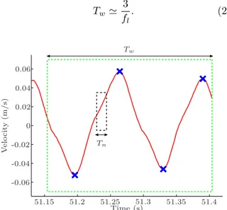
in the vibration index. At a given time, only the vibrations inside the wide time window are consid-ered. Figure 3 illustrates the concept of wide time window. The width of the wide time window may be adjusted depending on the applications. The authors suggest a minimum time frame of
Tw' 3 fl . (2) Tw V e lo c it y (m / s) Time (s) Tn 0 0.02 -0.02 0.04 -0.04 0.06 -0.06 51.15 51.2 51.25 51.3 51.35 51.4
Figure 3: Illustration of the wide and narrow time win-dows: the green dashed lines represent the boundaries of the wide time window while black dashed-dot lines represent the boundaries of a narrow time window at a given point in the wide time window.
3.3. Narrow time window
130
In order to characterize the vibration level, all the signal minima and maxima within a wide time window are identified. To this end, one possible approach would be to find the zeros of the signal derivative. However, in practice, the signal is too
135
noisy and this approach cannot be applied. There-fore, the narrow time window technique is pro-posed. It consists in using a narrow window of duration Tn to scan each point in the wide time
window from the beginning to the end. The
nar-140
row time window is centred on the point to be tested and this point is registered if it is a maximum or minimum within the narrow time window.
The duration of the narrow time window Tn is
large number of minima and maxima will be found due to signal noise. On the other hand, if it is too large, high frequency vibrations will not be de-tected. Indeed, one has
Tn<
1 2fh
(3)
where fh is the highest frequency to be accounted
for in the vibration index. The choice of Tn is
145
largely dependent on the signal noise.
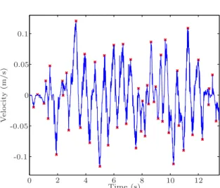
Figure 3 shows a wide-time window and a nar-row time window. Figure 4 shows the minima and maxima obtained with a low-noise signal while Fig. 5 shows the results obtained with a noisy
sig-150
nal, demonstrating the algorithm’s robustness to noise.
In mathematical terms, the signal is discretized using a sampling period Ts, which leads to j = TTns+
1 signal samples, noted si, i = 1, . . . , j, where si is
the magnitude of the signal corresponding to the ith sample. The magnitude of the signal for the sample corresponding to the centre of the narrow window, noted sc, with c =2TTn
s is then considered.
If one has
sc = max(s1, . . . , sj) (4)
then a maximum is detected while if
sc= min(s1, . . . , sj) (5)
a minimum is detected. Otherwise, no extremum is detected. Finally, if both a maximum and a mini-mum are detected for a given point, the latter is
ig-155
nored. This narrow time window test is performed for each point in the wide time window.
It should be pointed out that the narrow time window does not scan the wide time window at each time step. Instead, it is possible to use the
160
results from the preceding wide time window to re-duce computational costs.
At this point in the algorithm, a series of minima and maxima of a given signal have been obtained with robustness in regards to noise.
165
3.4. Vibration index
Based on the minima and maxima detected in a given wide time window, a vibration index (V ) is proposed. First, the total number of extrema, noted q, is computed. If there are fewer than two extrema,
170
the index is set to zero. Otherwise, the following definition is proposed for the vibration index:
V = λ q−1 X i=1 |y1,i+1− y1,i| (t1,i+1− t1,i) (6) 0.15 V e lo c it y (m / s) Time (s) 0 0 0.05 -0.05 0.1 -0.1 0.5 1 1.5 2 2.5 3 3.5 4
Figure 4: Minima and maxima detected by the algorithm for a low-noise signal (Tn= 0.03s). V e lo c it y (m / s) Time (s) 0 0 0.05 -0.05 0.1 -0.1 2 4 6 8 10 12
Figure 5: Minima and maxima detected by the algorithm for a noisy signal (Tn= 0.3s).
where y1,i and t1,i are respectively the signal
am-plitude and the time corresponding to the ith ex-tremum and λ is a scaling factor. The latter is only
175
used to scale the index, for simplicity of use. The larger the difference between two consecutive extrema, the larger the index will be. Similarly, the shorter the time between two consecutive extrema, the larger the index will be. In other words, an
180
increase in vibration amplitude or frequency results in a higher vibration index.
A modified version of the index may include lim-its on the index’s rate of change. A rising limit (Lr) and a falling limit (Lf) are used to smooth
185
the vibration index in order to avoid abrupt varia-tions. A saturation can also be applied to prevent the vibration index from increasing indefinitely.
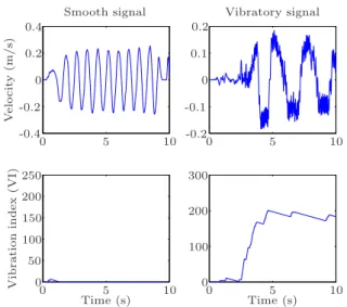
Figure 6 shows an example of the determination of the vibration index. On the left hand side, the
190
signal is taken from a smooth human-robot inter-action situation while on the right hand side the signal is taken from a stiff interaction, leading to vibrations. Smooth signal V e lo c it y (m / s) Vibratory signal V ib ra ti o n in d e x (V I) Time (s) Time (s) 0 0 0 0 0 0 0 0 0.1 -0.1 0.2 0.2 -0.2 -0.2 0.4 -0.4 5 5 5 5 10 10 10 10 50 100 100 150 200 200 250 300
Figure 6: Example of the determination of the vibration in-dex, V , for two signals taken from a human-robot interaction experiment. On the left hand side with a smooth interaction situation and on the right hand side with a stiff interaction leading to vibrations (Tw = 0.25s, Tn = 0.03s, λ = 20, Lr= 12.5s−1, Lf = 0.5s−1)
4. Application to admittance control
195
This section first recalls the concept of admit-tance control and then presents the implementation of the vibration observer-controller.
4.1. Admittance control
Two main control classes are used in haptics and pHRI namely, impedance and admittance con-trol [20]. Impedance controllers accept a dis-placement as input, which is measured, and react with a force. Devices controlled by this method should ideally have low inertia and friction since the user will inevitably feel these forces if they are not adequately compensated for. Admittance con-trollers, on the other hand, accept a force as in-put, which is measured, and react with a displace-ment [21, 22, 23]. Applications involving moder-ately large payloads usually use admittance control where a handle or a force/torque sensor is normally used to detect human intentions [24, 2, 23]. Ad-mittance control is detailed in [23, 25, 1]. The one-dimensional admittance equation is written as:
fH= m¨x + c ˙x. (7)
where fH is the interaction force, i.e., the force
ap-200
plied by the human operator, m the virtual mass, c the virtual damping and x, ˙x, ¨x are respectively the position, velocity and acceleration.
The trajectory to be followed by the robot can be prescribed as a position xd or as a desired velocity
˙
xd. For velocity control, the desired velocity can be
written, in the Laplace domain, as:
˙ Xd(s) = FH(s) ms + c = FH(s)/c m cs + 1 = FH(s)H(s). (8)
where ˙Xd(s) is the Laplace transform of ˙xd, FH(s)
is the Laplace transform of fh and s is the Laplace
205
variable. Velocity control is used here, similarly to what was done in [26, 27, 23].
4.2. Admittance control with vibration observer-controller
Although stability issues pertaining to
210
impedance control have been vastly explored [28, 29, 30, 31], not much has been reported for admittance control [32, 33].
With admittance control, vibrations or instabil-ity may occur when facing a stiff environment (in
215
many cases the operator can be the source of stiff-ness.). In order to prevent such a situation — be-cause safety is the primary concern — admittance parameters are then normally set to very conser-vative values. Therefore, large operator forces are
220
required to move the device even under normal con-ditions.
The objective here is to set the admittance pa-rameters to low values in order to be able to easily move the device. The vibrations generated from a
225
stiff environment can be eliminated by the vibration observer/controller. There is still a trade-off be-tween vibration and performance but the vibration controller is activated only when necessary and thus the trade-off is limited to exceptional situations.
230
5. Vibration controller
Once the level of vibrations are detected, the con-troller must be adapted in order to decrease or elim-inate the vibrations. The following section presents adaptive control strategies to achieve this goal along
235
with simulation results. The one degree-of-freedom (dof) system used in the simulations is shown in Fig. 7 where m and c are the admittance virtual mass and virtual damping, fH is the human force
input, vd is the desired velocity and v is the
de-240
vice velocity. The robot is represented as an inertia (Mr) with damping (Cr) and a PD controller is
used, with parameters K and Td.
+ -fH Admittance vd 1 ms+c Controller K(1 + Tds) Robot 1 Mr s+Cr x v
Figure 7: System used for the simulations.
5.1. Adaptive control strategies
Different control strategies are possible. In the
245
human-robot interaction context, it is proposed to adapt the admittance parameters, to add damping or to modify the PID controller gain. Each of these cases are described below.
5.1.1. Adaptive admittance parameters
250
Referring to the admittance equation, i.e., eqn. (7), if the admittance parameters (m and c) are low, the robot is easy to move but is also be more re-active to high-frequency inputs (for instance when interacting with a stiff environment). If the
param-255
eters are high, the robot is more difficult to move but also less reactive to high frequency inputs. In order to be robust to high frequency inputs and be-cause safety is the primary concern, the admittance parameters are normally set very high, thus
requir-260
ing large forces to move the robot. A main objec-tive of this research is to eliminate this compromise.
One possible approach is to set low admittance pa-rameters in normal operation and to increase the parameters when vibrations are detected. The
vir-265
tual mass and virtual damping must remain posi-tive in order for the admittance transfer function to remain stable and the parameters should not be modified too quickly to avoid exciting the system.
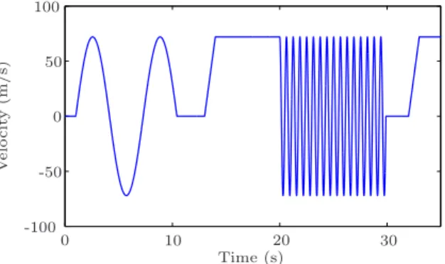
A force profile shown in Fig. 8 is sent to the
sys-270
tem as input. The first part (0 − 13s) is a low fre-quency sinusoidal signal, the second part is a con-stant input (13 − 20s), the third part is a high fre-quency sinusoidal signal (20−30s) and the last part is a constant input (> 30s). 275 Time (s) V e lo c it y (m / s) 0 0 10 20 30 50 -50 100 -100
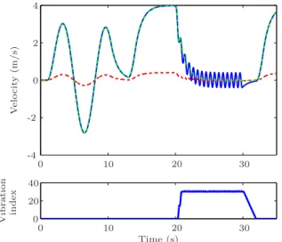
Figure 8: Force input profile used in the simulations. Figure 9 shows the resulting desired velocity with different admittance parameters as well as the re-sulting vibration index. With low admittance pa-rameters (m = 18, c = 18), the system reaches high velocities but is very reactive to high-frequency
in-280
puts. With high admittance parameters (m = 180, c = 180), the system only reaches small velocities and would require large forces to move but it is not very reactive to high-frequency inputs. With the vibration controller, the system reaches high
veloc-285
ities and is not very reactive to high-frequency in-puts. The parameters are varied linearly between [m = 18, c = 18] (when the index V is below 15 (Vmin)) and [m = 180, c = 180] (when the index V
is over 25 (Vmax)).
290
5.2. Adaptive damping
A common strategy to decrease vibrations is to add damping to the system. The principle is very simple and system stability is also easy to prove. However, there may be a practical limit of damping
295
that can be added due to signal noise and commu-nication delay. Since damping uses a signal deriva-tive, a special attention in the selection of the differ-entiation algorithm is important in order to avoid
V e lo c it y (m / s) Time (s) V ib ra ti o n in d e x 0 0 0 0 2 -2 4 -4 10 10 20 20 20 30 30 40
Figure 9: Desired velocity resulting from the force input shown in Fig. 8. The solid blue line is obtained with low admittance parameters (m = 18, c = 18). The red dashed line is obtained with high admittance parameters (m = 180, c = 180). The green dashed-dot line is obtained with the vibration controller (the parameters are varied between (m = 18, c = 18) and (m = 180, c = 180)). The second subplot shows the vibration index.
noise amplification, which can increase the
vibra-300
tions when the noise is transmitted to the actua-tors [34].
5.3. Adaptive controller
When faced with a stiff environment, robotic sys-tems using admittance control tend to exhibit more
305
vibrations when high loop gains are used. The con-trol parameters can be set to lower values, but, as a compromise, the position or velocity would not follow the command as precisely. The objective here is to set high default controller gains but to
310
decrease the controller gains when vibrations are detected. A first advantage of this method over modifying the admittance parameters is that it is more general and it can be applied in a variety of situations. A second advantage is that modifying
315
the admittance parameters may not work in some specific cases. For example, if there is a pertur-bation on the output leading to vibrations (severe noise or sensor error), lowering the controller gains would help but modifying the admittance
parame-320
ters would not since it would only modify the ref-erence.
The closed-loop transfer function of the system
(see Fig. 7) can be written as:
v vd
= K(1 + Tds)
s(M + KTd) + (K + C)
. (9)
Therefore, the state velocity can be written as
vs= Sr· vd=
K
K + C · vd (10)
where Sr is defined as the steady state ratio. The
time constant is obtained as
τ = M + KTd
K + C . (11)
The first controller was chosen to minimize the error while remaining stable with Sr = 0.99 and
τ = 0.15, leading to K = 50000 and Td= 0.14. The
325
second controller was chosen to be less reactive to high frequency inputs with Sr= 0.55 and τ = 0.82,
leading to K = 500 and Td = 0.484. In order for
the system with the adaptive controller to remain stable, the system represented in eqn. (9) must
min-330
imally be stable for any K and Td obtainted from
the adaptive controller law [35]. The adaptive con-troller linearly modifies the parameters between the first controller (when the index V is below 5 (Vmin))
and the second controller (when the index V is over
335
15 (Vmax)) and always leads to stable systems. As a
general rule, the parameters should not be modified too quickly in order to avoid exciting the system.
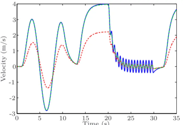
Figure 10 shows the measured velocity with dif-ferent control parameters for the force profile
in-340
put shown in Fig. 8. With high control gains (first controller), the system reaches high velocities but is very reactive to high-frequency inputs. With low control gains (second controller), the system only reaches small velocities and would require large
345
forces to move but is not very reactive to high-frequency inputs. Using the vibration controller, the system reaches high velocities and is not very reactive to high-frequency inputs.
5.4. Parameters summary
350
1
6. Prototypes
This section provides a brief description of the prototypes used for the experimental validation of the algorithms.
Time (s) V e lo c it y (m / s) 0 0 1 -1 2 -2 3 -3 4 5 10 15 20 25 30 35
Figure 10: Velocity resulting from the force input shown in Fig. 8. The solid blue line represents the desired velocity and also the measured velocity obtained with high control gains (the two curves are virtually superimposed). The red dashed line is the velocity with low control gains. The green dashed-dot line is the velocity with the vibration controller (the control parameters are adapted between the high and low control gains).
Table 1: Suggested parameter values
Parameter Value Tw 3/fl Tn 1/(2fh) λ 20 Lr Twλ Lf Tw·λ/20 Vmin λ/2 Vmax Vmin+ λ ηmin 0.02 Cooperation handle Force-torque sensor
Linear ball screw slide Mass
Motor
Figure 11: One DOF linear ball screw slide prototype.
6.1. One-DOF linear ball screw slider
The one-DOF linear ball screw slider is shown in Fig. 11. An ATI Mini-40 6-axis force/torque sensor is mounted between the end-effector and the han-dle. Only the force component along the direction
360
of motion of the slider is used for the experiments. The controller is implemented on a real-time QNX computer with a sampling period of 2ms which is enough high for avoiding instability coming from sampling during the experiment. The algorithms
365
are programmed using Simulink/RT-LAB software.
6.2. Prototype of a 4-DOF intelligent assist device The robot used for the second series of exper-iments reported in this paper is a prototype of a 4-dof intelligent assist device (IAD) [1], shown
370
in Fig. 12. This device allows three translations (XY Z) and a rotation (θ) about the vertical axis. In this prototype, the total moving mass is approx-imately 500kg in the direction of the X axis and 325kg along the Y axis. Additionally, the payload
375
may vary between 0 and 113kg. The horizontal workspace is 3.3m × 2.15m while the vertical range of motion is 0.52m. The range of rotation about the vertical axis is 120◦. These characteristics are summarized in Tab. 2. As the first prototype, the
380
controller is implemented on a real-time QNX com-puter with a sampling period of 2ms. The algo-rithms are programmed using Simulink/RT-LAB software.
Figure 12: Prototype of a 4-dof intelligent assist device.
7. Experimental validation
385
This section presents the experiments performed with the two prototypes described in the preced-ing section. In these experiments, velocity control
Table 2: Characteristics of the prototype of a 4-dof intelli-gent assist device.
X axis Y axis Z axis θ axis
Range 3.3m 2.15m 0.52m 120◦
Moving inertia 500kg 325kg 148kg 66kgm2
is used with a proportional controller and friction compensation. No derivative gain is used since the
390
signal is noisy (second derivative of the position) and no integral gain is used since the behaviour to a human input would then depend on the error his-tory [23].
A control ratio, η, is used to adapt the control gains and is defined as
η = ( ηmin if η0< ηmin η0 otherwise (12) where η0 = 1 if V ≤ Vmin 0 if V ≥ Vmax Vmax−V
Vmax−Vmin otherwise
(13)
and where Vmin and Vmax are respectively
mini-395
mum and maximum index values and ηmin is the
minimum control ratio value.
Both the proportional gain and the friction com-pensation output are multiplied by the control ratio η, namely
K = K∗η (14)
for the proportional controller and similarly for the friction compensation, where K∗is the default pro-portional gain and K is the actual propro-portional
400
gain. From Fig. 7 and eqn. (9), it is readily ob-served that the system is of the second order, hav-ing two real poles, and that it remains stable for η > 0. Vmin
When using a proportional controller, the
adap-405
tive law is fairly simple. With a more complex con-trol algorithm, a design parameter (concon-troller fre-quency for instance) could be simply multiplied by the control ratio η. An exemple of an adaptive law with a PD controller was shown in section 5.3.
410
7.1. One-DOF linear ball screw slider
The experiments were performed with the follow-ing parameters. Virtual mass m: 2 kg, Virtual
damping c: 60 Ns/m, Default Proportional gain K∗: 0.01, Wide time window Tw : 0.25s, Narrow
415
time window Tn : 0.03s, Rising Limit : 12.5 s−1,
Falling Limit : 0.5 s−1, Minimum control ratio ηmin
: 0.02, Minimum index value Vmin : 17, Maximum
index value Vmax : 34, Scaling factor λ : 20.
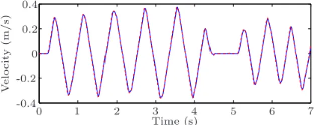
Figure 13 shows an example of a low frequency
420
interaction. This test was repeated using the vi-bration observer-controller and the results are the same with or without the controller. Indeed, no vi-brations are detected and the vibration controller is thus not activated.
V e lo c it y (m / s) Time (s) 0 0 0.2 -0.2 0.4 -0.4 1 2 3 4 5 6 7
Figure 13: Low frequency interaction. The solid blue line is the measured velocity while the red dashed line is the desired velocity.
425
Figure 14 shows an example of interactive ex-periment without the vibration observer-controller. The operator’s intention was to move the device at approximately 0.2m/s (which is a slow human arm speed) while being stiff. Both the desired and
mea-430
sured velocity include significant vibrations and the interaction is very uncomfortable.
V e lo c it y (m / s) Time (s) 0 0 0.2 -0.2 1 2 3 4
Figure 14: Stiff interaction without vibration observer-controller. The solid blue line is the measured velocity while the red dashed line is the desired velocity. This is not an unstable behaviour but a marginally stable situation which cannot be solve by using PO/PC.
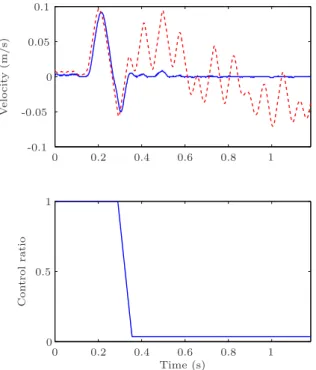
Figure 15 shows an example using the vibration observer-controller. The intention of the human op-erator was to stay at a given position while being
435
stiff and trying to minimally perturb the system. It can be observed that after one oscillation, after a very short period of time, the device is stabilized.
V e lo c it y (m / s) C o n tr o l ra ti o Time (s) 0 0 0 0 0.05 -0.05 0.1 -0.1 0.2 0.2 0.4 0.4 0.5 0.6 0.6 0.8 0.8 1 1 1
Figure 15: Stiff interaction around a given point with the vibration observer-controller. For the velocity subplot, the solid blue line is the measured velocity while the red dashed line is the desired velocity. The control ratio, equal to η, is the attenuation gain applied to the proportional controller and friction compensation output.
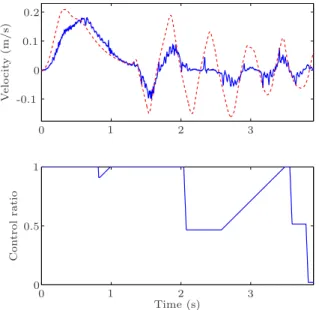
Figure 16 shows another example with the vi-bration observer-controller. The intention of the
440
operator was to move the device at approximately 0.5m/s (which is a moderate human arm speed) while being stiff. The interaction is very stable and there is no vibration. The same interaction without vibration controller leads to significant vibrations.
445
However, in this case, as soon as vibrations are de-tected, the control gains are reduced. The device’s velocity does not reach the desired velocity but the interaction is smooth and safe.
V e lo c it y (m / s) C o n tr o l ra ti o Time (s) 0 0 0 0 0.5 0.5 -0.5 1 2 2 4 4 6 6 8 8 10 10
Figure 16: Stiff interaction with vibration observer-controller. For the velocity subplot, the solid blue line is the measured velocity while the red dashed line is the de-sired velocity.
7.1.1. Passivity observer
450
The data obtained from the experiment shown in Fig. 14 was also monitored with a passivity ob-server (PO) [11] and Fig. 17 shows the PO output (energy). This kind of observer has been used suc-cesfully in many applications. However, it can be
455
observed here that the energy does not become neg-ative. In other words, the passivity controller (PC) does not detect any problem and would not apply any correction since it would not be activated. In-deed, the PO detects extra energy injected into the
460
system by non-passive behaviour while it does not detect vibrations that are due to a stiff but passive environment.
Time (s) P O o u tp u t (e n e rg y , J o u le s) 0 0 2 4 6 8 12 10 10 20 30
Figure 17: Passivity observer output with a stiff environ-ment.
7.2. 4-DOF intelligent assist device
Experiments were also performed with a 4-DOF
465
Intelligent Assist Device (only one axis (Y ) is re-ported for simplicity). This experiment provides a demonstration of the algorithm’s effectiveness on a different system which is also of a very differ-ent scale. The following parameters were used in
470
the experiment. Virtual mass m: 9 kg, Virtual damping c: 30 Ns/m, Default Proportional gain K∗: 0.06, Wide time window Tw : 1s, Narrow time
window Tn: 0.25s, Rising Limit : 12.5 s−1, Falling
Limit : 0.5 s−1, Minimum control ratio ηmin: 0.02,
475
Minimum index value Vmin : 3, Maximum index
value Vmax : 20, Scaling factor λ : 20.
Figure 18 shows an example of a stiff interaction without the vibration observer-controller. Both the desired and measured velocity include significant
vi-480
brations and the interaction is very uncomfortable. Figure 19 shows an example of stiff interaction with the vibration observer-controller. The intention of the human operator was to stay at a given position while trying to minimally perturb the system. It
485
can be observed that the device was stabilized.
V e lo c it y (m / s) Time (s) 0 0 0.5 -0.5 5 10 15 20 25
Figure 18: Stiff interaction without the vibration observer-controller. The solid blue line is the measured velocity while the red dashed line is the desired velocity.
V e lo c it y (m / s) C o n tr o l ra ti o Time (s) 0 0 0 0 0.1 -0.1 0.2 0.5 1 1 1 2 2 3 3
Figure 19: Stiff interaction around a point with the vibration observer-controller. For the velocity subplot, the solid blue line is the measured velocity while the red dashed line is the desired velocity. The control ratio, equal to η, is the attenuation gain applied to the proportional controller and to the friction compensation output.
Discussion
The algorithm was implemented on two proto-types. When interacting with a stiff environment, it has been shown that vibrations are very significant.
490
By using the vibration observer and controller, the device follows the operator’s intentions while elim-inating or reducing vibrations. The trade-off is to decrease the task performance (the measured ve-locity does not reach the amplitude of the desired
495
velocity for instance). However, the vibration con-troller is only activated when the vibrations are above a given treshold (both in frequency and am-plitude) and therefore it does not influence the per-formance in normal operation.
500
Conclusion
In this paper a time-domain vibration observer and controller applied to physical Human-Robot Interaction (pHRI) was proposed. An observer detecting minima and maxima from a given
sig-505
nal with robustness in regards to noise was first presented. A vibration index based on these ex-trema was then defined. This index was then used by an adaptive controller in order to reduce the vibrations. The algorithm was implemented on
two different prototypes to demonstrate its perfor-mance. Future studies will focus on adaptive con-trol laws for more complex concon-trollers and on sta-bility proofs.
Acknowledgements
515
This work was supported by The Natural Sci-ences and Engineering Research Council of Canada (NSERC) as well as by General Motors (GM) of Canada.
References
520
[1] C. Gosselin, T. Laliberte, B. Mayer-St-Onge, S. Fou-cault, A. Lecours, V. Duchaine, N. Paradis, D. Gao, R. Menassa, A friendly beast of burden: A human-assistive robot for handling large payloads, IEEE Robotics Automation Magazine 20 (4) (2013) 139–147.
525
doi:10.1109/MRA.2013.2283651.
[2] J. E. Colgate, M. Peshkin, S. H. Klostermeyer, Intel-ligent assist devices in industrial applications: a re-view, in: Proceedings of the International Conference on Intelligent Robots and Systems, 2003, pp. 2516–
530
2521. doi:10.1109/IROS.2003.1249248.
[3] R. Bischoff, J. Kurth, G. Schreiber, R. Koeppe, A. Albu-Schaeffer, A. Beyer, O. Eiberger, S. Haddadin, A. Stemmer, G. Grunwald, G. Hirzinger, The KUKA-DLR lightweight robot arm - a new reference platform
535
for robotics research and manufacturing, 41st Interna-tional Symposium on Robotics (2010) 1 –8.
[4] E. Guizzo, E. Ackerman, The rise of the robot worker, IEEE Spectrum 49 (10) (2012) 34–41. doi:10.1109/ MSPEC.2012.6309254.
540
[5] http://www.universal-robots.com/, visited May 02, 2014.
[6] A. M¨ortl, M. Lawitzky, A. Kucukyilmaz, M. Sezgin, C. Basdogan, S. Hirche, The role of roles: Physical cooperation between humans and robots, The
Interna-545
tional Journal of Robotics Research.
[7] Y. Li, K. P. Tee, W. L. Chan, R. Yan, Y. Chua, D. Limbu, Continuous role adaptation for human robot shared control, Robotics, IEEE Transactions on 31 (3) (2015) 672–681.
550
[8] M. Erden, A. Billard, Hand impedance measurements during interactive manual welding with a robot, IEEE Transactions on Robotics 31 (1) (2015) 168–179. [9] R. Adams, B. Hannaford, Stable haptic interaction with
virtual environments, IEEE Transactions on Robotics
555
and Automation 15 (3) (1999) 465 – 74.
[10] J. Gil, A. Avello, A. Rubio, J. Florez, Stability analy-sis of a 1 dof haptic interface using the routh-hurwitz criterion, IEEE Transactions on Control Systems Tech-nology 12 (4) (2004) 583–588. doi:10.1109/TCST.2004.
560
825134.
[11] B. Hannaford, J.-H. Ryu, Time-domain passivity con-trol of haptic interfaces, Transactions on Robotics and Automation 18 (1) (2002) 1 – 10. doi:10.1109/70. 988969.
565
[12] J.-H. Ryu, D.-S. Kwon, B. Hannaford, Stability guaran-teed control: Time domain passivity approach, Trans-actions on Control Systems Technology 12 (6) (2004) 860 – 868. doi:10.1109/TCST.2004.833648.
[13] H. C. Cho, J. H. Park, Stable bilateral teleoperation
570
under a time delay using a robust impedance control, Mechatronics 15 (5) (2004) 611 – 625. doi:http://dx. doi.org/10.1016/j.mechatronics.2004.05.006. [14] J.-H. Ryu, C. Preusche, Stable bilateral control of
teleoperators under time-varying communication delay:
575
time domain passivity approach, in: IEEE Interna-tional Conference on Robotics and Automation, Roma, Italy, 2007, pp. 3508 – 3513. doi:10.1109/ROBOT.2007. 364015.
[15] H. C. Cho, J. H. Park, Impedance control with
vari-580
able damping for bilateral teleoperation under time de-lay, JSME International Journal, Series C: Mechanical Systems, Machine Elements and Manufacturing 48 (4) (2006) 695 – 703. doi:10.1299/jsmec.48.695. [16] B. Hannaford, J.-H. Ryu, Time domain passivity
con-585
trol of haptic interfaces, in: IEEE International Con-ference on Robotics and Automation, Vol. 2, 2001, pp. 1863 – 1869. doi:10.1109/70.988969.
[17] S. Hirche, M. Buss, Passive position controlled telep-resence systems with time delay, in: American Control
590
Conference, Vol. 1, Denver, CO, United States, 2003, pp. 168 – 173.
[18] M. Fardad, B. Bamieh, A frequency domain analysis and synthesis of the passivity of sampled-data systems, in: IEEE Conference on Decision and Control, Vol. 3,
595
Nassau, Bahamas, 2004, pp. 2358 – 2363. doi:10.1109/ CDC.2004.1428749.
[19] D. Ryu, J.-B. Song, S. Kang, M. Kim, Frequency do-main stability observer and active damping control for stable haptic interaction, Control Theory Applications,
600
IET 2 (4) (2008) 261 –268. doi:10.1109/ROBOT.2007. 363772.
[20] C. Carignan, K. Cleary, Closed-loop force control for haptic simulation of virtual environments, Haptics-e 1 (2) (2000) 1 – 14.
605
[21] V. Hayward, K. Maclean, Do it yourself haptics: part i, IEEE Robotics Automation Magazine 14 (4) (2007) 88 –104. doi:10.1109/M-RA.2007.907921.
[22] R. v. d. Linde, Hapticmaster - a generic force con-trolled robot for human interaction, Industrial Robot:
610
An International Journal 30 (2003) 515–524. doi:doi: 10.1108/01439910310506783.
[23] A. Lecours, B. Mayer-St-Onge, C. Gosselin, Variable admittance control of a four-degree-of-freedom intelli-gent assist device, in: IEEE International Conference
615
on Robotics and Automation, Saint Paul, USA, 2012, pp. 3903–3908. doi:10.1109/ICRA.2012.6224586. [24] K. Kosuge, N. Kazamura, Control of a robot handling
an object in cooperation with a human, in: 6th IEEE International Workshop RO-MAN Proceedings., 1997,
620
pp. 142 –147. doi:10.1109/ROMAN.1997.646971. [25] A. Lecours, C. Gosselin, Computed-torque control of
a four-degree-of-freedom admittance controlled intelli-gent assist device, in: Experimental Robotics, Vol. 88 of Springer Tracts in Advanced Robotics, Springer
In-625
ternational Publishing, 2013, pp. 635–649.
[26] R. Ikeura, H. Inooka, Variable impedance control of a robot for cooperation with a human, in: Proceedings of the IEEE International Conference on Robotics and Automation, Vol. 3, 1995, pp. 3097–3102. doi:10.1109/
ROBOT.1995.525725.
[27] T. Tsumugiwa, R. Yokogawa, K. Hara, Variable impedance control with regard to working process for man-machine cooperation-work system, in: Proceed-ings of the IEEE/RSJ International Conference on
In-635
telligent Robots and Systems, Vol. 3, 2001, pp. 1564– 1569. doi:10.1109/IROS.2001.977202.
[28] H. T. Jung, Seul, Stability and convergence analysis of robust adaptive force tracking impedance control of robot manipulators, Vol. 2, 1999, pp. 635–640. doi:
640
10.1109/IROS.1999.812751.
[29] H. A. Zeng, G., An overview of robot force control, Robotica 15 (5) (1997) 473–482.
[30] D. Surdilovic, Robust control design of impedance con-trol for industrial robots, in: IEEE International
Con-645
ference on Intelligent Robots and Systems, 2007, pp. 3572–3579. doi:10.1109/IROS.2007.4399456.
[31] H. A.-C. Chien, M.-C., Adaptive impedance control of robot manipulators based on function approximation technique, Robotica 22 (4) (2004) 395–403. doi:10.
650
1017/S0263574704000190.
[32] T. Tsumugiwa, R. Yokogawa, K. Yoshida, Stability analysis for impedance control of robot for human-robot cooperative task system, in: International Conference on Intelligent Robots and Systems, Vol. 4, Sendai,
655
Japan, 2004, pp. 3883 – 8. doi:10.1109/IROS.2004. 1390020.
[33] V. Duchaine, C. Gosselin, Investigation of human-robot interaction stability using lyapunov theory, in: IEEE International Conference on Robotics and
Automa-660
tion, 2008, pp. 2189 –2194. doi:10.1109/ROBOT.2008. 4543531.
[34] A. Ditkowski, A. Bhandari, B. Sheldon, Computing derivatives of noisy signals using orthogonal functions expansions, Journal of Scientific Computing 36 (3)
665
(2008) 333–349. doi:10.1007/s10915-008-9193-9. [35] D. Liberzon, A. Morse, Basic problems in stability
and design of switched systems, IEEE Control Systems 19 (5) (1999) 59–70. doi:10.1109/37.793443.