iii
Abstract
Climate change mitigation is one of the major challenges of our time. The anthropogenic greenhouse gases emissions have continuously increased since industrial revolution leading to global warming. A broad portfolio of mitigation technologies has to be implemented to fulfill international greenhouse gas emissions agreements. Some of them comprises the use of the underground as a storage of various substances. In particular, this thesis addresses the dynamics of carbon dioxide (CO2) and hydrogen (H2) underground storage.
Numerical models are a very useful tool to estimate the processes taking place at the subsurface. During this thesis, a solute transport in porous media module and various multiphase flow formulations have been implemented in COMSOL Multiphysics (Comsol, 2016). These numerical tools help to progress in the understanding of the migration and interaction of fluids in porous underground storages.
Three models that provide recommendations to improve the efficiency, monitoring and safety of the storages are presented in this manuscript: two in the context of carbon capture and storage (CCS) and one applied to underground hydrogen storage (UHS). Each model focus on a specific research question:
Multiphase model on CCS. The efficiency and long-term safety of underground CO2 storage depend on the migration and trapping of the buoyant CO2 plume. The wide range of temporal and spatial scales involved poses challenges in the assessment of the trapping mechanisms and the interaction between them. In this chapter a two-phase dynamic numerical model able to capture the effects of capillarity, dissolution and convective mixing on the plume migration is applied to a syncline-anticline aquifer structure. In anticline aquifers, the slope of the aquifer and the distance of injection to anticline crest determine the gravity current migration and, thus, the trapping mechanisms affecting the CO2. The anticline structure halts the gravity current and promotes free-phase CO2 accumulation beneath the anticline crest, stimulating the onset of convection and, thus, accelerating CO2 dissolution. Variations on the gravity current velocity due to the anticline slope can lead to plume splitting and different free-phase plume depletion time is observed depending on the injection location. Injection at short distances from the anticline crest minimizes the plume extent but retards CO2 immobilization. On the contrary, injection at large distances from anticline crest leads
iv
to large plume footprints and the splitting of the free-phase plume. The larger extension yields higher leakage risk than injection close to aquifer tip; however, capillary trapping is greatly enhanced, leading to faster free-phase CO2 immobilization.
Reactive transport model on convective mixing in CCS. Dissolution of carbon-dioxide
into formation fluids during carbon capture and storage (CCS) can generate an instability with a denser CO2-rich fluid located above the less dense native aquifer fluid. This instability promotes convective mixing, enhancing CO2 dissolution and favouring the storage safety. Convective mixing has been extensively analysed in the context of CCS over the last decade, however, the interaction between convective mixing and geochemistry has been insufficiently addressed. This relation is explored using a fully coupled model taking account the porosity and permeability variations due to dissolution-precipitation reactions in a realistic geochemical system based on the Hontomín (Spain) CCS pilot site project. This system, located in a calcite, dolomite, and gypsum bearing host rock, has been analyzed for a variety of Rayleigh and Damköhler values. Results show that chemical reactions tend to enhance CO2 dissolution. The model illustrates the first stages of porosity channel development, demonstrating the significance of fluid mixing in the development of porosity patterns. The influence of non-carbon species on CO2 dissolution shown in this study demonstrates the needs for realistic chemical and kinetic models to ensure the precision of physical models to accurately represent the carbon-dioxide injection process.
Multiphase model applied to seasonal UHS in northern Spain. A major disadvantage of
renewable energies is their fluctuation, that can lead to temporary mismatches between demand and supply. The conversion of surplus energy to hydrogen and its storage in the underground is one of the options to balance this energy gap. This study evaluates the seasonal storage of hydrogen produced from wind power in Castilla-León region (northern Spain). An actual saline aquifer is analysed by means of a 3D multiphase numerical model. Different extraction well configurations are explored during three years of injection-production cycles. Results demonstrates that underground hydrogen storage in saline aquifers can be operated with reasonable recovery ratios: a maximum hydrogen recovery ratio of 78%, which leads to a global energy efficiency of 30%, has been estimated. Upconing emerge as the major risk on saline aquifer storage; however, extraction wells located in the upper part of the aquifer can deal with its effects. Steeply
v
dipping geological structures appears as a critical requisite for an efficient hydrogen storage.
Keywords: Geological gas storage, Numerical modelling, Multiphase flow, Reactive
vii
Résumé
L'atténuation du changement climatique est l'un des défis majeurs de notre époque. Les émissions anthropiques de gaz à effet de serre ont augmenté de façon continue depuis la révolution industrielle, provoquant le réchauffement climatique. Un ensemble de technologies très diverses doivent être mises en œuvre pour respecter les accords internationaux relatifs aux émissions de gaz à effet de serre. Certaines d'entre elles ont recours au sous-sol pour le stockage de diverses substances. Cette thèse traite plus particulièrement de la dynamique du stockage souterrain du dioxyde de carbone (CO2) et de l'hydrogène (H2).
Des modèles numériques de transport réactif et multiphasiques ont été élaborés pour mieux comprendre la migration et les interactions des fluides dans des milieux poreux de stockage souterrain. Ils fournissent des recommandations pour améliorer l'efficacité, la surveillance et la sécurité du stockage. Trois modèles sont présentés dans ce document, dont deux dans le domaine du captage et du stockage du CO2 (CCS pour
Carbon Capture and Storage), et le troisième s'appliquant au stockage souterrain de
l'hydrogène (UHS pour Underground Hydrogen Storage). Chacun d'entre eux traite plus spécifiquement un aspect de la recherche :
Modèle multiphasique appliqué au CCS L'efficacité et la sécurité à long terme du
stockage du CO2 dépend de la migration et du piégeage du panache de CO2 flottant. Les grandes différences d'échelles temporelles et spatiales concernées posent de gros problèmes pour évaluer les mécanismes de piégeage et leurs interactions. Dans cet article, un modèle numérique dynamique diphasique a été appliqué à une structure aquifère synclinale-anticlinale. Ce modèle est capable de rendre compte des effets de capillarité, de dissolution et de mélange convectif sur la migration du panache. Dans les aquifères anticlinaux, la pente de l'aquifère et la distance de l'injection à la crête de l'anticlinal déterminent la migration du courant gravitaire et, donc, les mécanismes de piégeage affectant le CO2. La structure anticlinale arrête le courant gravitaire et facilite l'accumulation du CO2 en phase libre, en dessous de la crête de l'anticlinal, ce qui stimule la mise en place d'une convection et accélère donc la dissolution du CO2. Les variations de vitesse du courant gravitaire en raison de la pente de l'anticlinal peuvent provoquer la division du panache et une durée différente de résorption du panache en phase libre, qui dépend de l'endroit de l'injection. L'injection à faible distance de la crête de
viii
l'anticlinal minimise la taille du panache mais retarde l'immobilisation du CO2. Au contraire, l'injection à grande distance de la crête de l'anticlinal crée des panaches à empreinte étendue et leur division en plusieurs panaches en phase libre. Plus la distance à la crête est grande, plus le risque de fuite augmente. Cependant, elle favorise grandement le piégeage par capillarité, qui résulte en une immobilisation plus rapide du CO2 en phase libre.
Modèle de transport réactif sur les mélanges convectifs en CCS. La dissolution du
dioxyde de carbone dans des fluides de la formation pendant le captage et le stockage (CCS) peut générer une instabilité lorsqu’un fluide riche en CO2 plus dense se trouve au-dessus du fluide de moindre densité existant dans l'aquifère. Cette instabilité favorise le mélange convectif, augmente la dissolution du CO2 et va dans le sens d'une meilleure sécurité du stockage. Le mélange convectif a été largement étudié dans le domaine du CCS durant la dernière décennie, mais les interactions entre le mélange convectif et la géochimie restent insuffisamment traitées. Cette relation est examinée à l'aide d'un modèle totalement couplé, qui prend en compte les variations de porosité et de perméabilité dues aux réactions de dissolution-précipitation dans un système géochimique réaliste, sur la base du projet relatif au site CCS potentiel à Hontomín, en Espagne. Ce système se trouve dans une roche hôte constituée de gypse, de dolomite et de calcite. Il a été analysé et de nombreuses valeurs Rayleigh et Damköhler ont été relevées. Les résultats montrent que les réactions chimiques tendent à accroître la dissolution du CO2. Le modèle illustre les premières étapes du développement d'un chenal de porosité, ce qui démontre l'importance du mélange convectif dans le développement de motifs de porosité. L'influence de composés inorganiques sur la dissolution du CO2 constatée dans cette étude, démontre le besoin de modèles cinétiques et chimiques réalistes, permettant aux modèles physiques de représenter avec précision le processus d'injection du dioxyde de carbone.
Modèle multiphasique appliqué à l'UHS saisonnière dans le nord de l'Espagne. L'un
des plus grands inconvénients des énergies renouvelables est qu'ils présentent des fluctuations, entraînant des déséquilibres entre la demande et l'approvisionnement en électricité. La transformation en hydrogène de l'énergie en excès et son stockage dans le sous-sol représente l'une des solutions pour y pallier. Cette étude évalue le stockage de l'hydrogène obtenu à partir de la production éolienne dans la région de
Castille-et-ix
León, dans le nord de l'Espagne. Un aquifère salin est analysé à l'aide d'un modèle numérique multiphasique en 3D. Différentes configurations de puits d'extraction sont étudiées sur une période de trois ans de cycles d'injection-production. Les résultats montrent que le stockage souterrain de l'hydrogène dans les aquifères salins peut être exploité avec des taux de récupération raisonnables. Un taux maximal de récupération de l'hydrogène de 78 % a été atteint, ce qui correspond à une efficacité énergétique globale de 30 %. Le risque majeur posé par le stockage en aquifère salin est l'intrusion, qui peut cependant être évitée en situant les puits d'extraction à proximité de la surface supérieure de l'aquifère. Des structures géologiques à fort pendage semblent constituer un critère essentiel d'efficacité d'un stockage d'hydrogène.
Mots clés: Stockage géologique du gaz, Modélisation numérique, Transport réactifs, Flux multiphasique, Captage au stockage du CO2, Stockage souterrain de l'hydrogen
xi
Acknowledgments
The research leading to this PhD. manuscript has received funding from the CO2-REACT People Programme (Marie Curie Actions) of the European Union's Seventh Framework Programme FP7-2012-ITN under REA grant agreement n° 317235.
I would like to thank my supervisors Dr. Fidel Grandia and Dr. Eric Oelkers for their encouragement, guidance and support. My sincere thanks to Dr. Elena Abarca and Albert Nardi for their constant help and exceptional interest on science and to the colleagues of the CO2-REACT ITN, especially to Martin Voigt and Christian Grimm who have guided and helped me with the endless paperwork at the university.
I also want to thank Roberto Martínez-Orío from IGME (Instituto Geológico y Minero de España) for his support in the collection of the geological data used in the section 3.2 of this manuscript.
Last but not least, I want to thank those who have accompanied me during the development of the thesis, from near or from afar, but always with trust, support and joy.
xiii
Table of contents
Abstract ... iii
Résumé ... vii
Acknowledgments ... xi
Table of contents ... xiii
List of figures ... xvii
List of tables ... xxiii
1 Introduction ... 1 Introduction en français ... 5 2 Numerical tools ... 9 Multiphase flow ... 9 2.1.1 Mathematical description ... 9 2.1.2 Numerical methods ... 18 2.1.3 Verification ... 22 Solute transport ... 33 2.2.1 Mathematical model ... 35 2.2.2 Numerical method ... 38 2.2.1 Verification: ... 39
Comments on the numerical tools ... 43
3 Carbon capture and storage ... 47
Carbon dioxide storage in porous media ... 47
Interactions of CO2 gravity currents, capillarity, dissolution and convective mixing in a syncline-anticline system. ... 51
3.2.1 Introduction ... 51
3.2.2 Model Description ... 52
xiv
3.2.4 Concluding remarks ... 64
Convective mixing fingers and chemistry interaction in carbon storage ... 67
3.3.1 Introduction ... 67
3.3.2 Model description ... 68
3.3.3 Results ... 75
3.3.4 Conclusions ... 83
4 Underground hydrogen storage ... 85
Hydrogen as energy storage from renewables ... 85
Quantitative assessment of seasonal underground hydrogen storage from surplus energy in Castilla-León (north Spain) ... 87
4.2.1 Introduction ... 87
4.2.2 Problem definition ... 89
4.2.3 Mathematical Model ... 92
4.2.4 Results and discussion ... 96
4.2.5 Conclusions ... 102
5 General conclusions and perspectives ... 103
Conclusions générales et perspectives en français ... 106
References ... 113
Annex I. Studies on early detection and impact of CO2 leakage. ... 137
A. Article on “Atmospheric dispersion modelling of a natural CO2 degassing pool from Campo de Calatrava (northeast Spain) natural analogue. Implications for carbon storage risk assessment” ... 139
B. Conference article on “Enhanced radon emission in natural CO2 flows in Campo de Calatrava region (central Spain)” ... 151
C. Conference article on “The effect of CO2 concentrations increase on trace metal mobility: a field investigation” ... 157
Annex II. Verification of the solute transport in porous media with iCP. ... 163
xv
B. Benchmark 2: Calcite dissolution and precipitation ... 164 C. Benchmark 3: Matrix-fracture oxygen intrusion ... 166 Annex III. Article on “convective mixing fingers and chemistry interaction in carbon storage” ... 169 Annex IV. Article on “Assessment of feasible strategies for seasonal underground hydrogen storage in a saline aquifer” ... 181
xvii
List of figures
Figure 1-1. Reprint of the Figure SPM.1 of the 5th IPCC Synthesis Report (Pachauri et al., 2014) showing evidences and other indicators of a changing global climate system. Observations: (a) Annually and globally averaged combined land and ocean surface temperature anomalies relative to the average over the period 1986 to 2005. Colours indicate different data sets. (b) Annually and globally averaged sea level change relative to the average over the period 1986 to 2005 in the longest-running dataset. Colours indicate different data sets. All datasets are aligned to have the same value in 1993, the first year of satellite altimetry data (red). Where assessed, uncertainties are indicated by coloured shading. (c) Atmospheric concentrations of the greenhouse gases carbon dioxide (CO2, green), methane (CH4, orange) and nitrous oxide (N2O, red) determined from ice core data (dots) and from direct atmospheric measurements (lines). Indicators: (d) Global anthropogenic CO2 emissions from forestry and other land use as well as from burning of fossil fuel, cement production and flaring. Cumulative emissions of CO2 from these sources and their uncertainties are shown as bars and whiskers, respectively, on the right hand side. The global effects of the accumulation of CH4 and N2O emissions are shown in panel c. ... 2
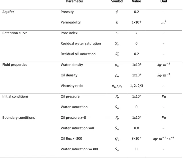
Figure 2-1. Conceptual model of the Buckley-Leverett problem. ... 23 Figure 2-2. Water saturation profile after 300 days of the Buckley-Leverett problem.
Viscosity ratios of 1, 2 and 2/3 are shown for the numerical and analytical solutions. . 23
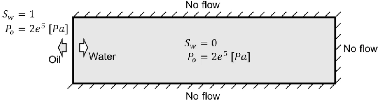
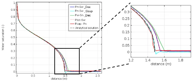
Figure 2-3. Conceptual model of the McWhorter problem. ... 25 Figure 2-4. Water saturation profile after 2.78 hours of the McWhorter problem. The
analytical and various numerical results are presented. The formulations are denoted by their dependent variables: wetting pressure (Pn), wetting pressure (Pw), non-wetting saturation (Sn), non-wetting saturation (Sw), global pressure (Ptot) and capillary pressure (Pcap). The suffix “Coup” and “Dec” denotes the coupled and decoupled pressure-saturation formulation respectively. ... 26
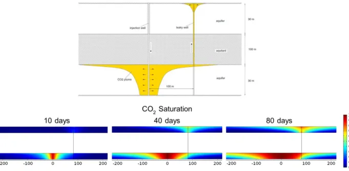
Figure 2-5. Conceptual model from Class et al. (2009) and modelling results of the CO2 plume for the problem A at 10, 40 and 80 days. ... 28
xviii
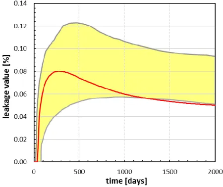
Figure 2-6. Leakage rates through leakage well for problem A. Model result (red) is
compared with the values obtained by various models in Class et al. (2009) (yellow area). ... 30
Figure 2-7. Leakage rates through leakage well for problem B. Model result (red) is
compared with the values obtained by various models in Class et al. (2009) (yellow area). ... 30
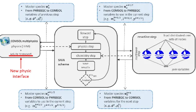
Figure 2-8. One step SNIA structure of iCP. The transport, potentially coupled with other
physical processes, is solved in the first step by COMSOL and the chemical reactions are solved in a second step by PHREEQC. The PHREEQC calculations are parallelized by iCP. The main variables transferred in each step are pointed. The implemented conservative solute transport module is highlighted. ... 35
Figure 2-9. GUI of the component solute transport module implemented in COMSOL.
The panel at the left show the solute transport module with the boundary and initial conditions available. The panel at the middle shows the equation solved and allow the user to assign the parameters and variables. The right panel shows the geometry of the model. The parts of the geometry where a physical process or boundary should be taken into account can be interactively selected. ... 38
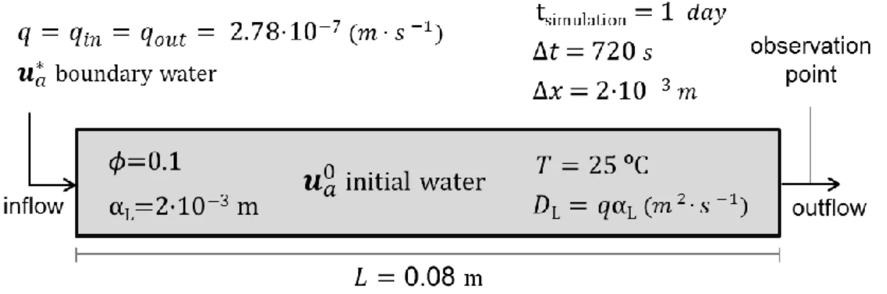
Figure 2-10. Physics and parameters of the Benckmark Problem 3: Cation Exchange. . 39 Figure 2-11. From left to right: NaX, CaX2 and KX exchanger fractions after 4h. Despite
the problem is 1D a 3D column is modelled for demonstation purposes. ... 40
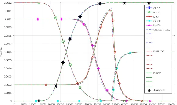
Figure 2-12. Comparison of the breacktrough curves of Cl, N, Na, K and Ca at the end of
the column. The results of PHREEQC, PHAST, CRUNCHFLOW and ICP are plotted. ... 41
Figure 3-1. Schematic illustration of the CO2 evolution in a saline dome-shape aquifer. Time increases downwards. The migration of free-phase CO2 as well as its dissolution in the native fluid and the consequent convective mixing are depicted. Dots represent the edges of free-phase plume: the trailing edge (TE, red) and leading edge (LE, blue). When the plume splits, an interior trailing edge (ITE, green) and interior leading edge (ILE, black) are defined. ... 48
Figure 3-2. Model geometry and boundary conditions. Hydrostatic pressure is assumed
at the lateral boundaries, while top and bottom of the aquifer are considered impervious. Three well locations (A, B and C) are considered in the simulations. ... 56
xix
Figure 3-3. Evolution of the CO2 mass in free-phase (a) and dissolved (b) after 1, 10, 25 and 100 years in a section of the model for injection in well B (located at coordinate 4000). The green colours in (a) correspond to capillary trapped CO2, while red and yellow are actual mobile free-phase. Note different scales and the log units on (a). ... 59
Figure 3-4. Vertically averaged concentration (1H 0H CCO2dz) of free-phase (a) and
dissolved (b) CO2 for the injection in well B at four simulation times. H is the thickness of the aquifer and CCO2 is the concentration of mobile (not trapped by capillarity) free-phase CO2 (a) and dissolved CO2 (b). Injection is located at 4000 m and anticline crest at 6000 m. Note that the vertical scale differs between the two plots. ... 60
Figure 3-5. Temporal and spatial evolution of the free-phase plume footprint for
injection in wells A, B and C. The extension of the gravity current is illustrated with the evolution of the plume edges (see Figure 3-1 for comprehensive meaning). The edges delimit the free-phase plume with vertical CO2 concentration larger than 2 kg·m-3 (Figure 3-4). The slope and depth of the aquifer top surface are illustrated on the top graphs for reference. From the injection point the mobile free-phase plume migrates updip towards the anticline crest. In the cases with injection in well A or B, the plume splits into two. Those cases have two more edges apart from the leading (LE, blue) and trailing (TE, red): the interior leading (ILE, green) and interior trailing (ITE, black) edge. The light oscillations on the LE are numerically generated during concentration integration. .... 61
Figure 3-6. Evolution of the CO2 injected with the contributions of different trapping mechanisms: structural, capillary and solubility for injection in wells A, B and C during 100 years. Two zooms of the figure are presented in a) first 3 years and b) 40 years with a smaller vertical scale. ... 63
Figure 3-7. Evolution of the share (%) between the trapping mechanisms: structural,
capillary and solubility during 100 years for injection in wells A, B and C. Note the log scale in the time axis. ... 64
Figure 3-8. Schematic illustration of the domain and boundary conditions considered in
this study. The migration of supercritical CO2 as well as its dissolution in the native brine promotes the convective mixing of the fluids. ... 73
Figure 3-9. Dimensionless carbon concentration (left) and horizontal average carbon
xx
simulation with Rayleigh = 3600 and Damköhler = 9.21x10⁶ (RaH-DaM). Note the arrows illustrate the fluid velocity field. Dimensionless carbon concentration is defined as: C' = (CT-CmaxT)/(CminT-CmaxT); where CminT and CmaxT represent the minimum and maximum carbon concentration in the simulation ... 76
Figure 3-10. Comparison of averaged CO2 flux per meter of aquifer lateral extent for all simulations and compared to the pure diffusion flux. RaH, RaM and RaL refer to high, medium and low Rayleigh number; DaH, DaM and DaL mean high, medium and low Damköhler number– see Table 3. Conservative refers to simulations without chemical reactions and equilibrium refers to simulations assuming calcite is in equilibrium with the fluid phase. The results of DaH and DaL are similar to the equilibrium and conservative simulations, respectively and in some cases their curves overlap. Both axis are in logarithmic scale. ... 77
Figure 3-11. Distribution of change in calcite content, change in gypsum content, pH,
calcium, sulphur and chlorine for the simulation with Rayleigh = 3600 and Damköhler = 9.21x10⁶ (RaH-DaM) after one year. Note the different scales and units. The changes in mineral content is illustrated in log scale, areas with no change in mineral content are shown in white... 78
Figure 3-12. Logarithm of porosity increase (left) and horizontal average percentage of
porosity variation (right) for the RaH-DaM simulation after one year. Areas with no increase are shown in white. The red circles close to the top indicate areas of porosity loss due to gypsum precipitation. ... 79
Figure 3-13. Vertical profile of spatially averaged density (a), porosity (b), pH (d) and
aqueous sulphur (d) for simulations with equal Rayleigh (3600) and different reactivity: high, medium and low Damköhler numbers (RaH-DaH, RaH-DaM and RaH-DaL), calcite in equilibrium (RaH-Eq) and conservative case (RaH-Cons); after one year of simulation. An inset in a shows a detail of the vertical profiles. Note the different units and vertical scales in b. ... 80
Figure 3-14. Time evolution of calcite dissolution rates (a) and calcite dissolution rates
versus gypsum precipitation rates (b) for all simulations. RaH, RaM and RaL refer to high, medium and low Rayleigh numbers; DaH, DaM and DaL stand for high, medium and low Damköhler numbers – see Table 3. Simulations with low Da (around 1.85x10⁴) are
xxi
difficult to distinguish in (a) due to their small dissolution flux. The slope of the linear regression between calcite dissolution and gypsum precipitation is plotted in (b). ... 81
Figure 3-15. Total dissolved carbon (a), maximum downward penetration of fingers (b)
and time of convection onset (c) versus Rayleigh number; and maximum porosity development (d) versus Damköhler number for all simulations after one year. In (d) values from simulations with high and medium Da are overlapped. Note the log scales in (c) and (d). The slopes of the linear regression between the axes are plotted in the figures. ... 82
Figure 4-1. Average electricity demand and wind energy production in Castilla-León
annual evolution in the period between 2013 and 2015. Data from REE-Red Electrica de España (2016). The location map shows Castilla-León region (brown) and the Burgos province (green)... 89
Figure 4-2. a) Top surface of the Utrillas formation, extension of the Spanish Tertiary
sedimentary basins, location of the San Pedro belt (red), drilled core (white) and limits of the numerical model. b) Stratigraphy of the NE margin of the Duero basin. The Utrillas sandstone formation is the target aquifer for hydrogen storage. Thicknesses of Tertiary cover in the thrust belts are largely decreased. Data extracted from Leon et al. (Leon et al., 2010). ... 91
Figure 4-3. Spatial discretization of the modelled 3D structure. A refined tetrahedral
grid is used in the axial part of the dome. Results are plotted focusing in this refined area. Blue limits indicate where Dirichlet conditions are imposed. ... 94
Figure 4-4. Utrillas formation at the axial area of the San Pedro dome and wells’ location:
Injection well and extraction well in case B well (white), horizontal extraction well in case A (yellow) and short vertical extraction wells in case C (black). The N-S cross-section is displayed in Figure 4-5. ... 96
Figure 4-5. Gas saturation in the upper part of the aquifer for the A case after second
year injection (a) and extraction (b). Injection well (white bar) and extraction well (yellow circle) are displayed. The cross-section plotted correspond to the N-S section in Figure 4-4. ... 97
Figure 4-6. vertically integrated H2 concentration over the aquifer thickness (kg ⋅ m-2) for the case A after: (a) first year injection, (b) first year extraction, (c) second year
xxii
injection, (d) second year extraction, (e) third year injection and (f) third year extraction. ... 98
Figure 4-7. Evolution of the total amount of H2 stored in the aquifer (a) and well injection and extraction rate (b) during operation for the three cases analysed. ... 99
Figure 4-8. Gas saturation evolution at the extraction well bottom and water extraction
mass flux (kg ⋅ s-1) during the first production cycle for case B if production well is not stopped. Upconing is evident after 35 days. ... 100
Figure 4-9. Total amount of H2 produced for the three years of operation and for all the cases. The percentage of H2 recovered (ration between the H2 produced and the H2 injected at the same year) is displayed on top of each column. ... 101
Figure 0-1: Comparison of the chloride breakthrough curves at the middle and end of
the column. The results of HP1, PHREEQC and iCP are plotted. ... 164
Figure 0-2: Comparison of the concentration of C, Ca, Cl, Mg, calcite and dolomite along
the column at the end of the simulation. The results of PHREEQC and iCP are plotted. ... 165
Figure 0-3. Conceptual model for oxygen intrusion along a fracture with adjacent
reducing rock matrix. The red rectangle delimits the domain modelled. Reprint of the Figure 7-1 of the (Sidborn et al., 2010) report. ... 166
Figure 0-4. Sketch of the numerical matrix-fracture oxygen intrusion model. ... 166 Figure 0-5. Dissolved tracer and oxygen concentrations in a vertical cut perpendicular to
the fracture direction at the coordinate x=0 after 5 days. The results of PHAST and iCP are compared... 168
xxiii
List of tables
Table 2-1. Buckley-Leverett model parameters. ... 24 Table 2-2. Brooks-Corey equations related to the retention curve. ... 24 Table 2-3. McWhorter model parameters. ... 27 Table 2-4. Characteristic values of the simulations of problems A and B. The table fields
are the same than tables 8 and 9 in Class et al. (2009). ... 29
Table 2-5. Well leakage model parameters. ... 31 Table 2-6. Cation exchange model parameters. ... 40 Table 2-7. Key features of iCP. Same fields as Tables 1 to 3 from Steefel et al. (2015) are
detailed... 45
Table 3-1. Thermodynamic relations ... 56 Table 3-2. Model parameters ... 56 Table 3-3. Chemistry of the two end-member fluids at 80ºC. Concentration in mmol·kgw -1. Density is given in kg·m-3. ... 70
Table 3-4. Model parameters. The calcite dissolution rate equation is taken from
Plummer et al. (1978), where 𝑘1, 𝑘2and 𝑘3are detailed. This equation is already implemented in the llnl database (Delany and Lundeen, 1990). 𝑎𝐻 +, 𝑎𝐶𝑂2and 𝑎𝐻2𝑂 correspond to the activity of protons, aqueous CO2 and water respectively... 74
Table 3-5. Description of Rayleigh and Damköhler numbers of various model
simulations. H= High, M= Medium and L= low... 75
Table 4-1. Model parameters. ... 95 Table 4-2. Summary of gas storage and energy efficiency values. % water mass
withdrawn is the ratio between the mass of water and the mass of H2 extracted; % energy recovered is the ratio between the energy re-electrified and the initial yearly surplus energy on Castilla-Leon; and % Burgos consumption is the ration between the energy re-electrified and the energy summer (Jun.-Sept.) consumption in Burgos. ... 101
Table 0-1: Transport of chloride model parameters. ... 163 Table 0-2: Calcite dissolution and precipitation model parameters. ... 165
xxiv
1
1 Introduction
Climate change mitigation is one of the major challenges of our time. The anthropogenic greenhouse gases emissions have continuously increased since the industrial revolution (Stocker et al., 2013), leading to global warming. Over the past decades, the atmosphere and ocean temperature have risen, the amount of snow and ice have diminished and sea level has increased, demonstrating unequivocally the warming of the climate systems (Figure 1-1) (Stocker et al., 2013). International agreements (European Commission, 2012, 2010; Kioto Protocol, 1997; Paris Agreement, 2015; Rio Summit, 1992) highlight the necessity to take climate protection actions.
A broad portfolio of technologies has to be implemented to mitigate global warming. The increase of renewable energy generation, the implementation of carbon capture and storage, the use of nuclear power and the improvement of energy efficiency are the most promising options to reduce greenhouse gases emissions (Edenhofer et al., 2014). Most of these, use subsurface environments as a storage of various substances (i.e. nuclear waste repositories, underground carbon reservoirs...). In particular, this thesis analyzes the dynamics of underground gas storage for carbon dioxide (CO2) and hydrogen (H2).
Carbon capture and storage (CCS) consist of capturing waste carbon dioxide from large point sources (i.e. fossil fuel power plants, cement industries...), transporting it and storing it into underground geological formations (Metz et al., 2005). The CO2 should be confined in the subsurface for a long time period (around 1000 years), preventing the release of carbon dioxide to the atmosphere. Underground hydrogen storage (UHS) comprises the injecting of a fluid (H2) into the subsurface as well, but in a different time scale. The purpose is to use hydrogen storage as grid energy storage. Hydrogen is a suitable energy vector that can be produced from surplus energy from renewables (energy generated that exceeds the immediate needs of the electricity grid); stored in the subsurface and extracted during periods of energy shortage. This can be used to balance the mismatches between energy demand and supply due to renewable energies fluctuation.
2
Figure 1-1. Reprint of the Figure SPM.1 of the 5th IPCC Synthesis Report (Pachauri et al., 2014) showing
evidences and other indicators of a changing global climate system. Observations: (a) Annually and globally averaged combined land and ocean surface temperature anomalies relative to the average over the period 1986 to 2005. Colours indicate different data sets. (b) Annually and globally averaged sea level change relative to the average over the period 1986 to 2005 in the longest-running dataset. Colours indicate different data sets. All datasets are aligned to have the same value in 1993, the first year of satellite altimetry data (red). Where assessed, uncertainties are indicated by coloured shading. (c) Atmospheric concentrations of the greenhouse gases carbon dioxide (CO2, green), methane (CH4, orange)
and nitrous oxide (N2O, red) determined from ice core data (dots) and from direct atmospheric
measurements (lines). Indicators: (d) Global anthropogenic CO2 emissions from forestry and other land
use as well as from burning of fossil fuel, cement production and flaring. Cumulative emissions of CO2
from these sources and their uncertainties are shown as bars and whiskers, respectively, on the right hand side. The global effects of the accumulation of CH4 and N2O emissions are shown in panel c.
Despite the differences in the ultimate goal of the storage and the consequent contrasting time scales, both underground storage efforts share many aspects. For
3
instance, the injection of a fluid phase in the subsurface, each with distinct physical and chemical properties than the native fluids, leads to the development of an interface between the phases with the subsequent capillary pressure. Factors such as the saturation or the effective permeability of the phases should be taken into account in multiphase flow conditions. Furthermore, the fluids injected in CCS and UHS operations are less dense and viscous than the native fluids; leading to their upward migration. An impervious overlaying seal is, thus, needed to ensure the confinement of the fluid within the geological formation. Other characteristics including high permeability, sufficient porosity and large volume capacity, which is indeed the main reason for considering underground storages, should be fulfilled by the underground storage structures. These similarities allow the transfer of knowledge from the extensively investigated carbon capture and storage field to the less mature field of underground hydrogen storage. The dynamics of the gas once injected in the subsurface and their impact on the host aquifer are complex to monitor since storage formations are generally found at large depths (>500 m) hindering fluid and rock analysis through time. The alternative, although being very expensive, is time-lapse geophysics such as electrical tomography, magnetotelluric and seismic methods. Such limitations in these data acquisition methods makes predictive numerical models a very useful tool to estimate the processes taking place at the subsurface. In this work, the fate of injected gases in porous media will be analysed using multiphase and reactive transport numerical models.
The development of this thesis comprised the improvement of several computational tools. A solute transport in porous media module and various multiphase flow formulations have been implemented in COMSOL Multiphysics (Comsol, 2016). The solute transport module has been tailored to meet the necessities of the reactive transport code iCP (Nardi et al., 2014a). iCP integrates COMSOL and PHREEQC (Parkhurst and Appelo, 2013), allowing the simulation of complex thermo-hydro-mechanical-chemical (THMC) processes. These tools have been, then, used to better understand the migration and interaction of fluids in porous underground storages; providing recommendations to improve the efficiency, monitoring and safety of the storages. The thesis has been divided into five chapters. Chapter 2 describes the numerical tools implemented during this thesis. The mathematical and numerical approaches applied
4
are explained together with some verification examples. Chapter 3 deals with the dynamics of CO2 in the subsurface in the context of CCS projects. It includes two sections: the first analyses the interactions of CO2 gravity currents, capillarity, dissolution and convective mixing using a miscible multiphase model; the second evaluates the influence of reactions on convective mixing fingers and CO2 dissolution using a fully coupled reactive transport model. Chapter 4 is focused on the storage of hydrogen produced from surplus energy in Castilla-León (north Spain). This chapter estimates the amount of H2 that can be recovered from an aquifer applying an immiscible two-phase model. Finally, the major findings of the research, together with some general conclusions and future perspectives are presented in Chapter 5.
In addition to the numerical models of underground gas storage presented in chapters 3 and 4, other activities have been developed in the course of this thesis as an effort to better understand the challenges and risks of the options to mitigate the climate change. Special efforts have been made on the analysis of natural occurring CO2 fluxes arriving to the surface. These systems give insights on the migration of CO2 at the near surface and atmosphere and on its effects on the ecosystems. Three studies based on field sampling aiming to evaluate monitoring techniques for the early detection of CO2 leakages and risk assessment methodologies are presented in Annex I.
5
Introduction en français
L'atténuation du changement climatique est l'un des défis majeurs de notre époque. Les émissions anthropiques de gaz à effet de serre ont augmenté de façon continue depuis la révolution industrielle (Stocker et al., 2013), provoquant le réchauffement climatique. Durant les dernières décennies, les températures de l'atmosphère et des océans ont augmenté, les quantités de neige et de glace ont diminué et le niveau des mers a monté, démontrant sans équivoque le réchauffement du système climatique (Figure 1-1) (Stocker et al., 2013). Des accords internationaux (European Commission, 2012, 2010; Kioto Protocol, 1997; Paris Agreement, 2015; Rio Summit, 1992) insistent sur la nécessité d'agir pour protéger le climat.
De nombreuses technologies très diverses doivent être mises en œuvre pour atténuer le réchauffement climatique global. L'augmentation de la production d'électricité à partir d'énergies renouvelables, la mise en place du captage et du stockage du CO2, l'utilisation de l'énergie nucléaire et l'amélioration de l'efficacité énergétique sont les solutions les plus prometteuses pour la réduction des émissions de gaz à effet de serre (Edenhofer et al., 2014). La plupart d'entre elles utilisent des sites souterrains pour le stockage de diverses substances (comme les sites d'enfouissement des déchets nucléaires, les puits de carbone, etc.). Cette thèse traite plus particulièrement de la dynamique du stockage gazier souterrain pour le dioxyde de carbone (CO2) et l'hydrogène (H2).
Le captage et stockage du CO2 (CCS) consiste à capter le dioxyde de carbone émis par de grandes sources (comme les centrales électriques à combustible fossile, les cimenteries, etc.), à le transporter et à le stocker dans des formations géologiques souterraines (Metz et al., 2005). Le CO2 doit être confiné dans le sous-sol pendant une longue période (de l’ordre de 1000 ans), empêchant ainsi sa libération dans l'atmosphère. Le stockage souterrain de l'hydrogène (UHS) consiste également à injecter un fluide (H2) dans le sous-sol, mais pour une période différente. Le but ici est de l'utiliser comme stockage d'énergie pour le réseau électrique. L'hydrogène convient comme vecteur énergétique parce qu'il peut être produit à partir des surplus d'électricité, elle-même produite à partir d'énergies renouvelables, lorsque la production dépasse les besoins immédiats du réseau. Il peut être stocké dans le sous-sol puis extrait pendant les périodes de pénurie.
6
Cela permet de pallier aux déséquilibres entre la demande et l'approvisionnement en électricité, dus aux fluctuations des énergies renouvelables.
Figure 1-1 Réimpression de la Figure SPM.1 du 5e rapport de synthèse du IPCC (Pachauri et al., 2014) on examine le rapport complexe entre les observations (panneaux a, b et c sur fond jaune) et les émissions panneau d sur fond bleu clair). Observations et autres indicateurs d’un système climatique planétaire en évolution. Observations: a) Moyenne annuelle et mondiale des anomalies de la température de surface combinant les terres émergées et les océans par rapport à la moyenne établie pour la période 1986–2005. Les différents ensembles de données sont représentés par des courbes de couleurs différentes. b) Moyenne annuelle et mondiale de l’évolution du niveau des mers par rapport à la moyenne établie pour la période 1986–2005 pour l’ensemble de données le plus long. Les différents ensembles de données sont représentés par des courbes de couleurs différentes. Tous les ensembles de données sont alignés par rapport à 1993, à savoir la première année de données d’altimétrie par satellite (courbe rouge). Lorsqu’elles sont estimées, les incertitudes sont représentées par des parties ombrées. c) Concentrations atmosphériques des gaz à effet de serre que sont le dioxyde de carbone (CO2, vert), le méthane (CH4, orange) et l’oxyde nitreux (N2O, rouge) déterminées à partir de l’analyse de carottes de glace (points) et obtenues par mesure directe dans l’atmosphère (courbes). Indicateurs: d) Émissions anthropiques mondiales de CO2 provenant de la foresterie et d’autres utilisations des terres ainsi que de l’utilisation des combustibles fossiles, de la production de ciment et de la combustion en torchère. Les cumuls des émissions de CO2 provenant des deux types de sources en question et les incertitudes qui y correspondent sont représentés par les boîtes à moustaches verticales sur la droite. Les effets globaux des cumuls des émissions de CH4 et de N2O sont représentés sur le panneau c.
7
Malgré les différences de finalités du stockage et les différences d'échelles de temps qu'elles supposent, ces deux types de stockage ont des aspects communs. Par exemple, l'injection souterraine de fluides, chacun avec des propriétés physiques et chimiques différentes de celles des fluides natifs, entraîne la création d'une interface entre les phases, présentant alors une pression capillaire. Certains facteurs, tels que la saturation ou la perméabilité effective des phases, doivent être pris en compte dans les conditions de flux multiphasique. De plus, les fluides injectés dans les opérations de CCS ou d'UHS sont moins denses et moins visqueux que les fluides natifs, ce qui entraîne leur migration ascendante. Il faut donc une couverture hermétique imperméable pour assurer le confinement du fluide au sein de la formation géologique. Il faut aussi que les structures souterraines de stockage présentent d'autres caractéristiques, comme une perméabilité élevée, une porosité suffisante et une grande capacité en volume, l'une des principales raisons pour considérer le stockage en sous-sol. Ces ressemblances permettent un transfert de connaissances du domaine très étudié du captage et du stockage du dioxyde de carbone à celui du stockage souterrain de l'hydrogène, nettement plus récent. La dynamique des gaz après injection dans le sous-sol et son impact sur l'aquifère hôte sont très difficiles à surveiller car les formations aptes au stockage sont souvent à de grandes profondeurs (> 500 m), ce qui rend difficile l'analyse des fluides et des roches au cours du temps. Bien qu'elle soit très chère à mettre en œuvre, on peut avoir recours à la géophysique time-lapse, faisant appel, entre autres, à des méthodes de tomographie électrique, magnéto-telluriques et sismiques. Les limitations des méthodes d'acquisition de données sont telles qu'il est très utile de disposer de modèles numériques prédictifs pour évaluer les processus qui ont lieu dans le sous-sol. Le présent travail étudie ce qu'il advient des gaz injectés dans un milieu poreux, à l'aide de modèles numériques de transport réactif et multiphasiques.
L'élaboration de cette thèse suppose l'amélioration de plusieurs programmes de calcul. Un nouveau module pour le transport des solutés et autres formulations des flux multiphasiques ont été implémentées à COMSOL (Comsol, 2016). Le nouveau module pour le transport des solutés dans les eaux souterraines a été élaboré pour répondre aux nécessités du code de transport réactif iCP (Nardi et al., 2014a). iCP intègre COMSOL et PHREEQC (Parkhurst and Appelo, 2013), capables de simuler des processus thermo-hydro-mécaniques et chimiques (THMC) complexes. Ces outils ont permis de mieux
8
comprendre la migration et les interactions des fluides dans des milieux poreux de stockage souterrain, de fournir des recommandations pour améliorer l'efficacité, la surveillance et la sécurité du stockage.
La thèse a été divisée en cinq chapitres. Le chapitre 2 décrit les outils numériques implémentés au cours de cette thèse. Les approches mathématiques et numériques appliquées sont expliquées avec quelques exemples de vérification. Le chapitre 3 traite de la dynamique du CO2 dans le sous-sol, dans le contexte des projets CCS. Il comporte deux sections : la première, analyse les interactions entre courants gravitaires de CO2, la capillarité, la dissolution et le mélange convectif, à l'aide du modèle multiphasique de fluides miscibles, et la seconde évalue l'effet des réactions sur les digitations dans les mélanges convectifs et la dissolution du CO2, à l'aide de modèles de transport réactifs complètement couplés. Le Chapitre 4 traite plus spécifiquement du stockage de l'hydrogène produit à partir du surplus électrique en Castille-et-León, dans le nord de l'Espagne. Dans ce chapitre est estimée la quantité d'H2 qui peut être récupérée d'un aquifère en utilisant un modèle diphasique de fluides non miscibles. Les résultats les plus importants de cette étude ainsi que les conclusions générales et les perspectives sont présentées dans le chapitre 5.
En plus des modèles numériques de stockage souterrain de gaz présentés aux chapitres 3 et 4, d'autres activités ont été menées au cours de cette thèse, afin de mieux comprendre les défis posés par les solutions envisagées et les risques de leur application à l'atténuation du changement climatique. Des efforts particuliers ont été faits sur l'analyse des flux naturels de CO2 arrivant à la surface. Ces systèmes donnent une idée de la migration du CO2 à proximité de la surface et de l'atmosphère et sur ses effets sur les écosystèmes. Trois études basées sur l'échantillonnage sur le terrain visant à évaluer les techniques de surveillance pour la détection précoce des fuites de CO2 et des méthodologies d'évaluation des risques sont présentées à l'annexe I.
9
2 Numerical tools
In this section the numerical tools to deal with multiphase flow and solute transport in porous media implemented during the thesis are explained. The thesis focusses on the processes occurring at the aquifer scale (from 1x10⁻³ to 10 m). A continuum approach, where the microscale properties are averaged over a representative elementary volume (REV) is followed. The numerical tools are implemented in COMSOL (Comsol, 2016). The main characteristics of the multiphase flow are described first, followed by the explanation of the groundwater solute transport. Both sections present the same structure: the mathematical models are presented first with a description of the main approaches reported in the literature; then, the numerical methods applied in their implementation are explained; and finally, some verification examples of the formulations are presented.
Multiphase flow
Multiphase flow occurs when two or more distinct fluids coexisting are separated by a sharp interface. Each fluid is considered, then, as a phase with its own physical and chemical properties. Taking into account the contact angle between the phases in the presence of a solid phase (θ), the phases can be divided into wetting (θ < 90°) and
non-wetting (θ > 90°). Due to the surface tension, there is a pressure change between phases
defined with the capillary pressure (𝑃𝑐):
𝑃𝑐 = 𝑃𝑛𝑜𝑛−𝑤𝑒𝑡𝑡𝑖𝑛𝑔 − 𝑃𝑤𝑒𝑡𝑡𝑖𝑛𝑔 (2-1)
In the case where two fluids are miscible and no interface occurs between them, they are considered as part of the same phase and are called components. One phase can contain one or more components (e.g. a gas phase composed by CO2 and CH4) and each component can be present in one or more phases (i.e. CO2 can be present in a system as a gas or dissolved in liquid).
2.1.1 Mathematical description
The number of phases and components to be described in the governing equations depends on the system. This thesis is focused on applications where the natural systems are composed by two phases and two components. Three-phase flow models are applied mainly for water, oil and gas systems in the hydrocarbon industry. A complete
10
description of the three-phase flow can be found at Chen et al. (2006) and Peaceman (1977) among others.
The mathematical description of two-phase systems can be found in the literature (Bastian, 1999; Bear, 1972; Chen et al., 2006; Garcia, 2003; Hassanizadeh and Gray, 1979; Helmig, 1997); and it is comprehensively described in articles related to multiphase flow simulation codes: MUFTE (Assteerawatt et al., 2005), DUMUx (Flemisch et al., 2011), OpenGeoSys (Goerke et al., 2011; O. Kolditz et al., 2012b), PFLOTRAN (Lu and Lichtner, 2005), TOUGH2 (Pruess et al., 1999; Pruess and Spycher, 2007), CodeBright (Vilarrasa, 2012), HYTEC (Sin et al., 2017), ECLIPSE (ECLIPSE, 2004), ELSA (Nordbotten et al., 2009, 2004b), FEHM (Pawar et al., 2005), GPRS (Cao, 2002; Jiang, 2008), IPARS (Wheeler and Wheeler, 2001), COORES (Le Gallo et al., 2006; Trenty et al., 2006), MoReS (Farajzadeh et al., 2012; Wei, 2012) and RTAFF (Sbai, 2007).
The mathematical model can vary widely in each application depending on the specific questions to be answered, the relevant processes, and the time scale and length associated to those processes. This thesis does not consider the geomechanical effects and the heat conservation in the multiphase flow. Simplifications of the multiphase flow such as vertical equilibrium models (Nordbotten and Celia, 2006) or macroscopic percolation models (Cavanagh and Haszeldine, 2014) are found to greatly reduce the computational complexity of the system. These simplified models are out of the scope of this thesis. A review of these methods can be found in Bandilla et al. (2015), Celia et al. (2015) and Celia and Nordbotten (2009).
This section starts with the description of the more general compositional model, where mass transfer between phases is taken into account. The component mass conservation system of equations and the constitutive and state relations needed to solve the system are explained. Then, some immiscible formulations are presented. In systems where the component behavior is not relevant, the multiphase flow can be represented by immiscible formulations with a much lower computational cost.
2.1.1.1 Compositional model
The mass conservation of each component (𝜅) in a system with 𝛼 phases can be written as:
11
∑ 𝜕𝛼 𝑡(𝜙𝑆𝛼𝜌𝛼𝑚𝛼𝜅𝑀𝜅) = ∑ −∇ ⋅ (𝒒𝛼 𝜶𝜌𝛼𝑚𝛼𝜅𝑀𝜅− 𝜙𝑆𝛼𝜌𝛼𝑫𝜶⋅ ∇(𝑚𝛼𝜅𝑀𝜅)) + 𝑇𝛼𝜅+ 𝑄𝛼𝜅
(2-2) where 𝛼 denotes the fluid phase, 𝜙 is the porosity of the medium (𝑚3⋅ 𝑚−3), 𝑆𝛼 is the
phase saturation (𝑚3 ⋅ 𝑚−3), 𝜌𝛼 is the phase density (𝑘𝑔 ⋅ 𝑚−3), 𝑚𝛼𝜅 is the molality of
the 𝜅 component in the 𝛼 phase (𝑚𝑜𝑙 ⋅ 𝑘𝑔−1), 𝑀𝜅 is the component molar weight (𝑘𝑔 ⋅ 𝑚𝑜𝑙−1), 𝒒
𝜶 corresponds to the phase Darcy’s flow in its multiphase form (𝑚3⋅ 𝑚−2⋅
𝑠−1), 𝑫
𝜶 is the phase diffusion/dispersion tensor (𝑚2⋅ 𝑠−1), 𝑄𝛼𝜅 is the component mass
source term in the 𝛼 phase (𝑘𝑔 ⋅ 𝑚−3⋅ 𝑠−1) and 𝑇𝛼𝜅 is the component interphase mass
transfer term (𝑘𝑔 ⋅ 𝑚−3⋅ 𝑠−1).
The last four terms can be extended as: 𝒒𝜶 = −𝑘𝑘𝛼𝑟 𝜇𝛼 (∇𝑃𝛼 − 𝜌𝛼𝒈) (2-3) 𝑫𝛼 = 𝐷𝑚𝑰 + |𝒒𝜶|(𝛼𝐿𝑬(𝒒𝜶) + 𝛼𝑇𝑬⊥(𝒒 𝜶)) (2-4) 𝑄𝛼𝜅 = 𝑄 𝛼𝑀𝜅𝑚𝛼𝜅 (2-5) 𝑇𝛼𝜅 = 𝜙𝑆 𝛼𝜌𝛼𝑘𝑘𝑖𝑛𝜅 (𝑚̅ 𝛼𝜅 − 𝑚𝛼𝜅)𝑀𝜅 (2-6)
where 𝑘 is the permeability tensor (𝑚2), 𝑘𝛼𝑟 is the relative phase permeability (−), 𝜇𝛼 is
the phase dynamic viscosity (𝑃𝑎 ⋅ 𝑠−1), 𝑃𝛼 is the pressure (𝑃𝑎) and 𝒈 is the gravity vector
(𝑚 ⋅ 𝑠−2), 𝐷𝑚 is the species-independent molecular diffusion coefficient (𝑚2⋅ 𝑠−1),
𝛼𝐿and 𝛼𝑇 are, respectively, the longitudinal and transverse dispersivity (𝑚), |𝒒𝜶| is the
Euclidean norm of Darcy’s flow, 𝑬(𝒒𝜶) is the orthogonal projection along velocity and
𝑬⊥ = 𝑰 − 𝑬(𝒒
𝜶), 𝑄𝛼 is the phase mass source term (𝑘𝑔 ⋅ 𝑚−3 ⋅ 𝑠−1), 𝑘𝑘𝑖𝑛𝜅 (𝑠−1) is the
interphase mass transfer of component 𝜅 and 𝑚̅ 𝛼𝜅 (𝑚𝑜𝑙 ⋅ 𝑘𝑔−1) is the solubility limit of
component 𝜅 in the 𝛼 phase.
The system of equations in (2-2) has 2𝑁𝛼 + 𝑁𝛼𝑁𝜅 dependent variables: 2𝑁𝛼 from the
phase pressures and saturations and 𝑁𝛼𝑁𝜅 components molalities. The system is
constrained by the phase saturation equation, the 𝑁𝛼 phase mass fraction and (𝑁𝛼−
12 ∑ 𝑆𝛼 𝛼 = 1 (2-7) ∑ 𝑀𝑘𝑚 𝛼𝑘 𝑘 = 1 (2-8) ∑ 𝑇𝛼𝑘 𝛼 = 0 (2-9) ∑ 𝑄𝛼𝑘 𝑘 = 𝑄𝛼 (2-10)
Constitutive relations
To close the system (𝑁𝛼 − 1) capillary pressure relations needs to be taken into
account. Generally, the capillary pressure is described as function of the saturation of the higher wettability (Niessner and Helmig, 2007). The most common approaches of the capillary pressure are Brooks and Corey (1964) and van Genuchten (1980). Recently, a more complex model where capillary pressure is function of the specific interfacial area apart from the saturation has been developed (Niessner and Hassanizadeh, 2008); however, it has been rarely implemented in multiphase flow models (Tatomir et al., 2015). In the multiphase flow equations implemented in this thesis the user can define whether Brooks and Corey or Van Genuchten capillary approach is used.
Additional equations relate the phase density and viscosity with its pressure, temperature and composition. The influence of pressure and temperature in the liquid density and viscosity is limited, while gas phases present much more variability. Usually, experimental relationships are used to determine the density and viscosity of the components. In this thesis, apart from the relations already implemented in COMSOL (Comsol, 2016), the properties of the CO2-brine system implemented by Pruess and Spycher (2007) in TOUGH2 are incorporated. The gas density can also be determined following the ideal gas law and the Peng-Robinson equation of state (Robinson and Peng, 1978). Other relationship could be easily added by the user to the system.
The partitioning of components between the phases is usually considered in equilibrium, which is a reasonable assumption when the time scale of mass transfer is large compared to the time scale of flow. Compositional multiphase formulations based on local equilibrium are extensively described in the literature (Firoozabadi, 1999; Lu and Lichtner, 2005; Michelsen et al., 2008; Pruess et al., 1999). In gas-liquid systems the Henry’s law and the saturation vapor pressure are used to define the mole fraction in each phase.
13
If component partitioning is not described by equilibrium, a kinetic expression is used for the interphase mass transfer (equation 2-6). Several approaches are described in the literature. Van Antwerp et al. (2008) extended the dual domain approach for kinetic mass transfer during air sparing from the laboratory scale (Falta, 2003, 2000) to field scale. Niessner and Hassanizadeh (2009) developed a method where the interphase mass transfer was function of the mass balance of the specific interfacial area. Other authors use a lumped mass transfer rate calculated through the non-dimensional modified Sherwood number (𝑆ℎ) to solve the equation (Agaoglu et al., 2015; Imhoff et al., 1994; Miller et al., 1990; Powers et al., 1994, 1992; Zhang and Schwartz, 2000):
𝑘𝑘𝑖𝑛𝑘 = 𝑆ℎ𝐷𝑚
𝑑502 (2-11)
𝑆ℎ = 𝛼𝑅𝑒𝛽𝑆
𝛽𝛾 (2-12)
where 𝑘𝑘𝑖𝑛𝑘 is the kinetic mass transfer rate (𝑠−1), 𝑑50 is the mean size of the reservoir grains (𝑚), 𝑅𝑒 is the Reynold’s number (-), 𝑆𝛽 is the saturation of the 𝛽 phase and 𝛼, 𝛽, 𝛾
are dimensionless fitting parameters. This approach is followed in the compositional multiphase formulation implemented in this thesis.
Choice of primary variables and system of equations
Different linear combinations of equations and state variables can be used to diminish the stiffness of the compositional multiphase flow system (Binning and Celia, 1999; Chavent, 1981; Chen et al., 2000; Chen and Ewing, 1997a; Coats, 1980). The most classic approach is to sum over components and choose the so-called natural variables (pressure and saturation of the phases and molality of components) as dependent variables and apply a local variable switching depending on the phases present in each cell (Class et al., 2002; Coats, 1980; Lu and Lichtner, 2005; Pruess et al., 1999).
Phase disappearance is one of the major problems in multiphase flow simulation. It leads to the degeneration of the equation satisfied by the saturation, making natural variables inappropriate. Variable switching is able to cope with this process varying the dependent variables depending on the phases present in each cell. Nevertheless, this approach has some drawbacks as generates perturbations on the Newton iteration when phase changes occur and affect the structure of the Jacobian matrix (Lu et al., 2010).
14
Several alternative approaches are proposed in the literature where the dependent variables remain constant throughout the domain. Jaffré and Sboui (2010) use complementarity conditions. Abadpour and Panfilov (2009) allow the extension of saturation to negative values. Moreover, various combinations of dependent variables are described for two phase flow: liquid phase pressure and water mass concentration (Bourgeat et al., 2013); gas pressure and liquid pressure (Angelini et al., 2011); pressure, saturation and fugacities (Lauser et al., 2011); capillary pressure and gas pressure (Neumann et al., 2013);… Comparison between some of these methods can be found in literature (Gharbia et al., 2015; Lu et al., 2010; Masson et al., 2014; Neumann et al., 2013; Voskov and Tchelepi, 2012).
In this thesis, the compositional multiphase flow is implemented and applied to carbon capture and storage (section 3.2) using the natural variables as dependent variables. Water miscibility in the CO2 rich phase is low, on the order of one per cent (Spycher and Pruess, 2005). Therefore, water dissolution in supercritical CO2 is neglected, reducing the system of equations (2-2) to three. Thus, only one interphase mass transfer (𝑇𝑙𝐶𝑂2) has to be defined through the Sherwood number approach. No variable switching is applied and it is considered that the liquid phase remains throughout the system, even in small amounts. A new linear combination of the system of equations (2-2) is used to describe the three equations of the system:
𝜕𝑡(𝜙𝑆𝑙𝜌𝑙 + 𝜙𝑆𝑔𝜌𝑔) = −∇ ⋅ (𝒒𝒍𝜌𝑙 + 𝒒𝒈𝜌𝑔) + 𝑄𝑔+ 𝑄𝑙 (2-13) 𝜕𝑡(𝜙𝑆𝑙𝜌𝑙𝑚𝑙𝐶𝑂2𝑀𝐶𝑂2 + 𝜙𝑆𝑔𝜌𝑔) = −∇ ⋅ (𝒒𝒍𝜌𝑙𝑚𝑙𝐶𝑂2𝑀𝐶𝑂2+ 𝒒 𝒈𝜌𝑔− 𝜙𝑆𝑙𝜌𝑙𝑫𝒍⋅ ∇(𝑚𝐶𝑂𝑙 2𝑀𝐶𝑂2)) + 𝑄𝑙𝐶𝑂2+ 𝑄𝑔 (2-14) 𝜙𝑆𝑙𝜌𝑙𝜕𝑡(𝑚𝑙𝐶𝑂2𝑀𝐶𝑂2) − 𝑚 𝑙 𝐶𝑂2𝑀𝐶𝑂2𝜕 𝑡(𝜙𝑆𝑔𝜌𝑔) = −𝒒𝒍𝜌𝑙⋅ ∇(𝑚𝑙𝐶𝑂2𝑀𝐶𝑂2) + 𝑚 𝑙𝐶𝑂2𝑀𝐶𝑂2∇ ⋅ (𝒒𝒈𝜌𝑔) + ∇ ⋅ (𝜙𝑆𝑙𝜌𝑙𝑫𝒍⋅ (𝑚𝑙𝐶𝑂2𝑀𝐶𝑂2)) −𝑄𝑙(𝑚𝑙𝐶𝑂2 − 𝑚𝑙𝐶𝑂2,∗)𝑀𝐶𝑂2 − 𝑄𝑔𝑚𝑙𝐶𝑂2𝑀𝐶𝑂2 + 𝑇𝑙𝐶𝑂2 (2-15)
where 𝑚𝑙𝐶𝑂2,∗ is the external CO2 concentration. These equations are derived from: 1. the total mass conservation equation (2-13) obtained by summing over all
equations of system of equations (2-2);
2. an equation for the CO2 mass conservation (2-14) obtained by adding the equations for the CO2 component (𝜅 = 𝐶𝑂2) in both phases (𝛼 = 𝑙, 𝑔);
15
3. equation (2-15), derived by subtracting equation (2-13) multiplied by 𝑚𝑙𝐶𝑂2𝑀𝐶𝑂2 from the aqueous CO
2 mass conservation (equation (2-2) for 𝛼 = 𝑙 and 𝜅 = 𝐶𝑂2).
The dependent variables solved are liquid pressure (𝑃𝑙) in equation (2-13), gas saturation (𝑆𝑔) in equation (2-14) and dissolved CO2 molality (𝑚𝑙𝐶𝑂2) in equation (2-15).
The approaches followed to model the fluids density and viscosity, the relative permeability and capillary pressure are used-defined.
2.1.1.2 Immiscible formulations
In cases where no mass transfer between phases or when the behavior of the components is not relevant for the purpose of the model; the mass balance equations can be written for the bulk phase rather than for individual components. The phase mass conservation is achieved by summing equation (2-2) over components and assuming no internal component gradient (no diffusion-dispersion within the phases):
𝜕𝑡(𝜙𝜌𝛼𝑆𝛼) = −∇ ⋅ (𝜌𝛼𝒒𝜶) + 𝑄𝛼 (2-16)
where 𝑄𝛼 is the phase mass source term (𝑘𝑔 ⋅ 𝑚−3⋅ 𝑠−1). The Darcy’s flow is described in equation (2-3). The system of equations (2-16) has 2𝑁𝛼 unknowns that
can be solved taking into account the saturation constrain (equation2-7) and the (𝑁𝛼− 1) capillary pressure relations (equation 2-1).
As for the compositional formulation, various dependent variables and linear combinations of equations can be selected (Aziz and Settari, 1979; Binning and Celia, 1999; Chavent, 1981; Chen et al., 2000; Hassanizadeh and Gray, 1979). Some of the formulations described in the literature and implemented during the thesis are summarized below for the two-phase flow systems.
Coupled Pressure-Saturation formulation
In this formulation, the general system of two equations (2-16) is solved without any linear combination. One equation takes the phase pressure as the dependent variable, while the other solves the phase saturation. Integrating the Darcy’s velocity and taking wetting saturation (𝑆𝑤) and non-wetting phase pressure (𝑃𝑛) as unknowns the system is