Edited by: Ludovico Minati, Tokyo Institute of Technology, Japan Reviewed by: Lauren Jean O’Donnell, Harvard Medical School, United States Kenichi Oishi, Johns Hopkins University, United States Yu Zhang, McGill University, Canada *Correspondence: Pamela Guevara [email protected] Received: 09 March 2020 Accepted: 19 June 2020 Published: 10 September 2020 Citation: López-López N, Vázquez A, Houenou J, Poupon C, Mangin J-F, Ladra S and Guevara P (2020) From Coarse to Fine-Grained Parcellation of the Cortical Surface Using a Fiber-Bundle Atlas. Front. Neuroinform. 14:32. doi: 10.3389/fninf.2020.00032
From Coarse to Fine-Grained
Parcellation of the Cortical Surface
Using a Fiber-Bundle Atlas
Narciso López-López1,2, Andrea Vázquez1, Josselin Houenou3,4,5,6, Cyril Poupon3,
Jean-François Mangin3, Susana Ladra2and Pamela Guevara1*
1Faculty of Engineering, Universidad de Concepción, Concepción, Chile,2Universidade da Coruña, CITIC, Department of Computer Science and Information Technologies, A Coruña, Spain,3Université Paris-Saclay, CEA, CNRS, Baobab, Neurospin, Gif-sur-Yvette, France,4INSERM U955 Unit, Mondor Institute for Biomedical Research, Team 15 “Translational Psychiatry”, Paris, France,5Fondation Fondamental, Paris, France,6AP-HP, Department of Psychiatry and Addictology, School of Medicine, Mondor University Hospitals, DHU PePsy, Paris, France
In this article, we present a hybrid method to create fine-grained parcellations of the cortical surface, from a coarse-grained parcellation according to an anatomical atlas, based on cortico-cortical connectivity. The connectivity information is obtained from segmented superficial and deep white matter bundles, according to bundle atlases, instead of the whole tractography. Thus, a direct matching between the fiber bundles and the cortical regions is obtained, avoiding the problem of finding the correspondence of the cortical parcels among subjects. Generating parcels from segmented fiber bundles can provide a good representation of the human brain connectome since they are based on bundle atlases that contain the most reproducible short and long connections found on a population of subjects. The method first processes the tractography of each subject and extracts the bundles of the atlas, based on a segmentation algorithm. Next, the intersection between the fiber bundles and the cortical mesh is calculated, to define the initial and final intersection points of each fiber. A fiber filtering is then applied to eliminate misclassified fibers, based on the anatomical definition of each bundle and the labels of Desikan-Killiany anatomical parcellation. A parcellation algorithm is then performed to create a subdivision of the anatomical regions of the cortex, which is reproducible across subjects. This step resolves the overlapping of the fiber bundle extremities over the cortical mesh within each anatomical region. For the analysis, the density of the connections and the degree of overlapping, is considered and represented with a graph. One of our parcellations, an atlas composed of 160 parcels, achieves a reproducibility across subjects of ≈0.74, based on the average Dice’s coefficient between subject’s connectivity matrices, rather than ≈0.73 obtained for a macro anatomical parcellation of 150 parcels. Moreover, we compared two of our parcellations with state-of-the-art atlases, finding a degree of similarity with dMRI, functional, anatomical, and multi-modal atlases. The higher similarity was found for our parcellation composed of 185 sub-parcels with another parcellation based on dMRI data from the same database, but created with a different approach, leading to 130 parcels in common based on a Dice’s coefficient ≥0.5.
1. INTRODUCTION
The human connectome is of special interest in understanding the brain structure and function (Toga et al., 2012). The structural connectome is composed of two basic elements, the somas (nodes) and the axons (edges) that exist between them, formed by white matter (WM) tracts (Sporns et al., 2005; Hagmann et al., 2007; Bullmore and Sporns, 2009). Magnetic Resonance Imaging (MRI) provides in-vivo techniques to study the human brain. MRI modalities include diffusion-weighted MRI (dMRI) that estimates the WM tracts of the brain (Mori and Barker, 1999), structural MRI (sMRI) which focuses on brain anatomy (Haacke et al., 1999), and functional MRI (fMRI) that estimates brain function (Huettel et al., 2004; Van Den Heuvel and Pol, 2010). dMRI allows researchers and clinicians to non-invasively study and in-vivo how white matter is organized in the brain giving details of its connectivity and structure (Le Bihan et al., 2001). It is based on measurements of the movement of hydrogen atoms present in water molecules of biological tissues. Tractography algorithms reconstruct an estimate of the main WM tracts of the entire brain based on dMRI information (Basser et al., 2000; Zhang et al., 2014). The generated datasets represent an estimation of the main WM pathways, in the format of 3D polylines, also called fibers, even though they do not represent real neural fibers (Mori and van Zijl, 2002; Perrin et al., 2005). This technique is indirect, and relies on models and inference, but allows a whole-brain exploration of WM structure in living humans, on large populations of subjects.
The structural networks of the human cerebral cortex have not yet been comprehensively mapped (Sporns et al., 2005; Hagmann et al., 2010; Toga et al., 2012). The brain’s structural and functional systems have features of complex networks, such as “small-world” topology, highly connected hubs and modularity, at the whole human brain scale (Bullmore and Sporns, 2009). The study of brain connectivity, taking into account its function and structure, can be performed based on a cortex parcellation, which is the cortical division of the brain into macroscopic regions (de Reus and Van den Heuvel, 2013). A parcellation may be based on resting state fMRI (rs-fMRI) (Schaefer et al., 2017), anatomical structure (Destrieux et al., 2010), dMRI (Lefranc et al., 2016), or cytoarchitecture. Architectonic and other template-based atlases have been created (Tzourio-Mazoyer et al., 2002; Desikan et al., 2006), but may not reflect the individual variations in regional functional boundaries. Data-driven parcellations can overcome this limitation through a better definition of individual cortical regions (Sotiropoulos and Zalesky, 2017). Parcellation atlases can be constructed using information from multiple modalities, and several scales. For example, for a given population, information from cortical folding, myelin content, resting-state, and task-based fMRI was integrated to create a functionally relevant parcellation (Glasser et al., 2016). However, individual variability and the limitations of each modality make the application of those methods very difficult. Here, we focus on the development of a method for the tractography-based parcellation (TBP) of the cortical surface. The method could be posteriorly integrated to multimodal parcellation frameworks (Parisot et al., 2017).
Connectivity-based methods use tractography information to find regions with common connectivity patterns between the cortical voxels, or cortical surface mesh vertices, that compose each region. All the methods have to deal with the high inter-subject variability, especially in the brain cortex and superficial white matter (SWM). Therefore, to reduce the complexity of the problem, some methods are focused or have been tested on a few brain regions, or have used an anatomical parcellation for initial regions (Anwander et al., 2006; Klein et al., 2007; Guevara et al., 2008; Perrin et al., 2008; Roca et al., 2010; Li et al., 2017). In general, the similarity between the connectivity profiles of the voxels (or vertices) is estimated using some similarity measure and then, a method is applied to regroup elements with common connectivity patterns. Some methods have been proposed to perform an analysis over the whole-brain cortex (de Schotten et al., 2014; Moreno-Dominguez et al., 2014; Parisot et al., 2015; Lefranc et al., 2016; O’Muircheartaigh and Jbabdi, 2017). This kind of approach, in general, calculates the whole connectivity profile of each seed node (image voxels or mesh vertices), followed by the computation of a connectivity matrix and clustering of the nodes. A group of methods performs a tractography-based parcellation of the cortex using only connectivity information given by the fiber extremities (Parisot et al., 2015; Lefranc et al., 2016; Li et al., 2017), while other groups embed fiber shape information into the analysis (de Schotten et al., 2014; Moreno-Dominguez et al., 2014; O’Muircheartaigh and Jbabdi, 2017). For an inter-subject analysis, it is also necessary to find the correspondence between subjects. One strategy is to create the parcellation taking into account the main connections present in the population of subjects (Schiffler et al., 2017). Another approach is to detect individual connectivity patterns, or even parcels, from the tractography of each subject and to then find consistent parcels among the population of subjects (Moreno-Dominguez et al., 2014; Lefranc et al., 2016; Li et al., 2017). Furthermore, due to the high complexity and the huge size of connectivity data, all the methods use a dimension reduction criterion. The difficulties mentioned above, among others, make the parcellation of the human brain cortex a complicated and unachievable task. In the following, we briefly describe some methods to provide an insight into the complexity of the solution implementation.
An interesting approach of whole-brain TBP is based on hierarchical clustering (Moreno-Dominguez et al., 2014). The method selects GM/WM interface voxels as seeds and generates probabilistic tractography from them. For each seed voxel a tractogram is obtained (visitation map). Hierarchical clustering is applied over the tractograms using a non-centered variant of the Pearson’s correlation coefficient as a similarity measure. The resulting dendrogram is post-processed to reduce the number of branchings. Next, a leaf-matching is iteratively applied to the two tractograms with the highest similarity, to find correspondence across subjects. Even though the method is promising, the different parameters were difficult to adjust and no perfect match was found.Lefranc et al. (2016)apply a watershed to the connectivity profiles averaged from all the subjects of a gyrus (patch) in order to split the cortical surface into catchment basins (Roca et al., 2009). A set of regions of interest strongly connected
to the gyrus across subjects is then identified, and a joint patch connectivity matrix across subjects is calculated. Finally, to construct the final cortex parcellation, each gyrus is clustered using the classical k-medoids algorithm applied to the distance matrix. The method removes a large part of the connectivity data by filtering, however, a good reproducibility among subjects was obtained. Another interesting example is the work proposed by O’Muircheartaigh and Jbabdi (2017). The method first calculates connectivity matrices from cortical vertices and subcortical voxels to the rest of the brain, based on probabilistic tractography. Then, creates an average matrix across the subjects and applies independent component analysis (ICA) to provide a group-average connectivity matrix. The dimensionality of this matrix is incrementally reduced in tractography space using principal component analysis (PCA) on subsets of the matrix. A post-processing is applied to obtain a hard parcellation of the cortex, without a straightforward mapping to tractography and gray matter, due to the high cortical and connectivity variability between subjects.
A different strategy for creating a parcellation is to use a hybrid method involving the use of bundles segmented from a bundle atlas. The first proof of concept used a subset of bundles manually selected from a multi-subject SWM bundles atlas (Guevara et al., 2017b). This work processed 10 subjects, using fix parameters manually tuned for all the processing. It segmented the bundles for each subject and calculated the intersection regions of the bundles with the cortex. In case of overlapping between two regions, the parcel label of the smaller parcel prevailed over the bigger one. This very preliminary work showed the potential advantage of using labeled bundles for the cortical parcellation, with relatively good correspondence in some regions of the brain. This method was then further improved by the use of a graph representation of the overlap between regions (Silva et al., 2019). This first attempt tuned the parameters in one subject and subsequently applied them to four other subjects, giving some correspondence across the subjects. However, since no inter-subject analysis is performed for the merging of the connecting regions, the method is not applicable to a large group of subjects. Extending this idea, we therefore propose a new hybrid method for the structural connectivity-based parcellation of the cortical surface, based on segmented bundles. Unlike most of the methods proposed in the literature, which use full tractography, we use fibers labeled into bundles, according to short and long bundle atlases. The advantage is that the correspondence of connecting regions is given in advance for the different subjects in a database. Furthermore, the generation of parcels from segmented bundles could provide a better representation of the main regions or nodes of the human brain connectome, since these were identified as the main short and long connections of the brain, represented in the atlases of bundles. The resulting parcellation will then represent a subdivision of the cortex into the regions that connect the most probable bundles. The method still experiences difficulty in clearly defining the nodes (cortex parcels), knowing that the bundles from tractography are very variable across subjects and may not exist in several subjects. This poses a big but interesting challenge. The key point of the proposed work is the automatic analysis of the
density and variability of the connecting regions among subjects over the cortical mesh, so that the most probable ones are selected, merged, and homogenized. The overlapping is solved using a graph representation of the intersected regions, taking into account the degree of overlapping of their density centers, across subjects.
The method was applied to a group of 79 subjects from a HARDI database. Several quantitative and qualitative evaluations were performed. Twenty parcellations were generated, based on different sets of the three parameters of the method, and compared to evaluate the similarity between them. Furthermore, a reproducibility analysis was also performed, based on the similarity of connectivity matrices across subjects, constructed with the whole tractography.
A comparison with a macro anatomical parcellation using Dice’s coefficient between subject’s connectivity matrices was performed, showing a slightly better reproducibility in a resultant parcellation generated with the proposed method. Moreover, other comparisons were also made with state-of-the-art parcellations based on different MRI modalities, finding a degree of similarity with dMRI, functional, anatomical, and multi-modal atlases. A higher similarity was found for our parcellation composed of 185 sub-parcels with another parcellation containing 239 parcels, based on dMRI data from the same database, but was created with a totally different approach. This comparison led to 130 parcels being in common based on a Dice’s coefficient ≥0.5 and 75 parcels being in common with a Dice coefficient ≥ 0.6. Finally, complementary analyses were performed that are included in a Supplementary File.
2. MATERIALS AND METHODS
2.1. Tractography Dataset
We used the ARCHI database (Schmitt et al., 2012), containing anatomical MRI and HARDI data from 79 healthy subjects with special acquisition sequences of a 3T MRI scanner with a 12-channel head coil (Siemens, Erlangen). The MRI protocol included the acquisition of a T1 image dataset using a MPRAGE sequence (160 slices, TE/TR = 2.98/2300 ms, TH = 1.10 mm, deflection angle FA = 9, TI = 900 ms; matrix = 256 × 240; voxel size = 1 × 1 × 1.1 mm; RBW = 240 Hz/pixel), a single-shell HARDI SS-EPI dataset along 60 optimized DW directions, and a field map B0, b = 1,500 s/mm2, (70 slices, TE
= 93 ms, FA = 90, TH = 1.7 mm, TR = 14,000 ms, matrix = 128 × 128, partial Fourier factor PF = 6/8, echo spacing ES = 0.75 ms, RBW = 1,502 Hz/pixel; GRAPPA = 2, total scan time = 16 min and 46 s). The database has the affine transformation matrices to convert the data between the spaces T1, T2 (diffusion space), and Talairach. By using the software BrainVISA/Connectomist-2.0 (Duclap et al., 2012), all data were pre-processed. The main artifacts, such as noise, susceptibility effects, geometric distortions, and eddy currents were corrected. Further, defective slices were removed. The analytic Q-ball model was also computed (Descoteaux et al., 2007). Whole-brain streamline deterministic tractography was calculated, using a T1-based brain propagation mask (Guevara et al., 2011a), with one seed per voxel at T1 resolution, a maximum curvature angle
of 30◦, and a tracking step of 0.2 mm. Resulting tractography
datasets contain about 1 million fibers per subject.
2.2. Approach
We propose a hybrid method for the creation of fine-grained parcellations of the cortical surface, from a coarse-grained parcellation according to an anatomical atlas, based on structural connectivity information, given by segmented bundles for a population of subjects. The bundle segmentation is based on atlas bundles from three different atlases. The parcellation method receives as an input tractography and the labeled mesh of each subject, the fused bundle atlas with selected superficial and deep white matter bundles. The method returns an average parcellation atlas for the input dataset, which consists of a subdivision of the anatomical parcels (gyri) of Desikan-Killiany atlas, based on the most stable connectivity-based sub-parcels across the subjects. The data consists of the labels associated with each cortical mesh vertex. Note that the cortical meshes used, based on Freesurfer processing output, contain the same number of triangles and vertices in all the subjects. For all the subjects, corresponding triangles will represent the same anatomical region, but with local differences, according to the morphology of each subject. To create the final parcellation, the method uses the probability and density information of the sub-parcels from all the subjects. An intermediate output of the method is therefore the probabilistic representation of each sub-parcel. Figure 1 shows a schematic of the parcellation method. The selection of the final bundle atlas is performed as a pre-processing stage (A). Next, the method is composed of six steps: (B) fiber bundle segmentation, (C) extraction of meshes and labels, (D) intersection of the fibers with the mesh, (E) fiber filtering, (F) cortex parcellation, and (G) sub-parcel post-processing.
2.2.1. Pre-processing: Fusion of Atlases
This pre-processing aims to create a fused atlas of white matter bundles, containing the main WM connections across subjects and, consequently, to create a more complete parcellation of the cortex (see Figure 1A). We used two atlases of superficial white matter (SWM) and one atlas of deep white matter (DWM). The first SWM atlas, swm_atlas_1, is composed of 50 bundles in both hemispheres, with a total of 7,857 fibers (Guevara et al., 2017a). The second SWM atlas swm_atlas_2, has 44,345 fibers and is made up of 44 bundles in the left hemisphere and 49 bundles in the right hemisphere (Román et al., 2017). Finally, the DWM atlas contains 18 bundles per hemisphere, corresponding to 11,755 fibers (Guevara et al., 2012). Those atlases were created using the ARCHI database, representing the most reproducible bundles across subjects (see Figure S2).
The bundles from both SWM atlases are labeled following the same naming convention, based on the anatomical regions of the Desikan-Killiany atlas (Desikan et al., 2006). The name contains lh or rh to denote the left or right hemisphere, followed by the name of the two regions connected by the bundle, according to the abbreviation of the region (see Table S3). Finally, a correlative number is added to indicate the index, as many bundles can connect the same two anatomical regions in an
atlas. For example, a bundle connecting the post-central and pre-central gyri of the left hemisphere is called: lh_PoC-PrC_0, where 0 is the index given by the atlas. The swm_atlas_1 contains only bundles connecting two different anatomical regions (gyri), while the swm_atlas_2 also contains bundles connecting different areas of an anatomical region. On the other side, the DWM atlas labels the bundles according to an abbreviation of their anatomical name, followed by LEFT or RIGHT to denote the hemisphere.
To fuse the atlases, we first analyzed the bundles that are very similar in both SWM atlases, connecting the same regions. In general, in the case of a high similarity between bundles from both atlases, we selected the most compact bundle. After a visual comparison of both atlases, the bundles of the swm_atlas_1 are better defined in their ends, and therefore are more suitable for performing a cortical parcellation. Some bundles with high similarity in both SWM atlases are shown in Figure S1. All the bundles of the swm_atlas_1 were therefore selected (see the first row of Figure S2). Next, 27 bundles in the left hemisphere and 34 in the right hemisphere for the swm_atlas_2 were selected, as shown in the second row of Figure S2. Most of the selected bundles of the swm_atlas_2 connect different areas within an anatomical region.
Respecting the DWM atlas, we first discarded the Corticospinal Tract, Fornix, and Thalamix Radiations, as those bundles do not represent cortico-cortical connections. We also discarded the Corpus Callosum as it is a very large bundle that would not be very informative for the definition of subdivisions of the anatomical regions. The selected bundles are: Arcuate fasciculus, with its anterior and posterior portions (AR, AR_ANT, AR_POST), Cingulum (CG), Inferior Fronto-Occipital (IFO), Inferior Longitudinal (IL), and Uncinate (UN) bundles (see the third row of Figure S2). These bundles cover the cortical regions that the two SWM atlases do not cover, achieving a complete coverage of the cortex. The fused atlas is in MNI space and contains a total of 179 bundles, distributed in 86 bundles in the left hemisphere (see Table S1) and 93 bundles in the right hemisphere (see Table S2), as we see in Figure S3 (first row).
Finally, the centroid of each atlas bundle is calculated as the mean of the corresponding points of all the fibers in a bundle, to later align the segmented fibers.
2.2.2. Step 1: Fiber Bundle Segmentation
This step performs the segmentation of white matter bundles for each subject (see Figure 1B). Segmenting the fibers provides direct correspondence of the bundles and the connected cortical regions across the subjects. The segmentation algorithm (Vázquez et al., 2019) is a parallel version of the algorithm proposed in Guevara et al. (2012). It classifies the fibers of a subject’s tractography based on a multi-subject WM bundle atlas. It calculates the maximum Euclidean distance between corresponding points of each subject fiber and each atlas fiber. A subject’s fiber is labeled with the closest bundle, if the distance does not exceed the maximum threshold defined for the bundle. The algorithm returns the subject’s fibers that were correctly classified, labeled with the corresponding bundle name. Figure S3shows the final atlas of white matter bundles as well as a subject segmented with the atlas.
FIGURE 1 | Schematic of the parcellation method. (A) Pre-processing: fusion of atlases. The bundles of a long and two short WM bundle atlases are fused into a final fiber bundle atlas. (B) Step 1: fiber bundle segmentation. A segmentation algorithm is applied to classify the fibers of each subject’s tractography with respect to the final fiber bundle atlas. (C) Step 2: Extraction of meshes and labels. By using FreeSurfer and then BrainVISA software, the cortical meshes and their corresponding labels, according to Desikan-Killiany atlas, are obtained. (D) Step 3: intersection of the fibers with the mesh. This step intersects the fibers of each subject with its cortical mesh, obtaining the initial and final triangles intersected by each fiber bundle. (E) Step 4: fiber filtering. The fiber bundles are filtered according to their anatomical definition, in order to discard the fibers connecting the wrong region. This algorithm first obtains the label of each intersected triangle, then removes misclassified fibers and then performs a fiber alignment according to the corresponding atlas bundle. (F) Step 5: cortex parcellation. This is the main step of the parcellation method. The objective is to subdivide each region (anatomical parcel) into sub-parcels based on probabilistic structural connectivity information, derivated from a set of segmented fiber bundles. The algorithm is divided into four sub-steps: (1) creating preliminary sub-parcels, (2) calculating probability maps, (3) processing sub-parcels, and (4) merging of candidate sub-parcels. Finally, a hard parcellation is obtained with the most probable label for each triangle of the cortical mesh. (G) Step 6: sub-parcel post-processing. To get more homogeneous parcels, the small connected components are eliminated, followed by a closing of the parcels over the cortex.
To perform the segmentation, the tractography datasets are resampled with 21 equidistant points, since it is a sufficient number to perform an analysis of the similarity between fibers, as used in others works (Guevara et al., 2011b, 2012). Before the calculation, the tractographies are transformed to the MNI space. This algorithm receives as an input the tractography of a subject, resampled with 21 equidistant points in MNI space, the fused bundle atlas, and the distance thresholds to be used for each bundle, defined for each original atlas (Guevara et al., 2012,
2017a; Román et al., 2017). It returns the segmented bundles for each subject, according to the labeling of the atlas bundles. 2.2.3. Step 2: Extraction of Meshes and Labels This step aims to obtain the meshes of the cortical surface and the labels of the anatomical regions given by the Desikan-Killiany atlas, as shown in Figure 1C. First, FreeSurfer software (Fischl, 2012) is employed to calculate the cortical surfaces for each subject. By using this software, a direct correspondence between
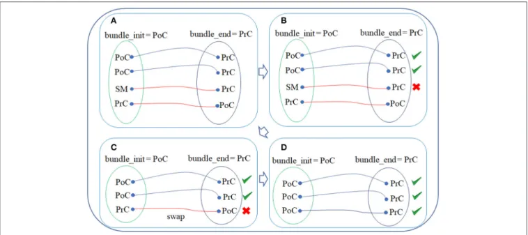
FIGURE 2 | WM fiber filtering for a bundle. (A) Sub-step 1: obtaining the fiber labels. The labels of the triangle vertices that are intersected by the start and end of each fiber are obtained. (B) Sub-step 2: removing of misclassified fibers. Fibers that were misclassified by respect to the bundle anatomical definition are discarded. (C) Sub-step 3: fiber alignment. The fibers that are stored in the inverse direction, by respect to the atlas bundle centroid, are inversed. (D) Filtered final fibers for a bundle.
the cortical surface mesh of the subjects is obtained, since the number of vertices is the same for all of them, changing only their 3D coordinates in the mesh according to the individual morphology. For the labeling of the cortical surface, FreeSurfer uses the Desikan-Killiany (DK) atlas, which consists of 35 regions per hemisphere (Desikan et al., 2006). Each region in the atlas (see Table S3) has associated a label (integer number). The labeling therefore consists of assigning each vertex of the mesh to the label of the region that it corresponds to. Next, BrainVISA software (Cointepas et al., 2010) was used to apply the pipeline that converts the formats and transforms the mesh to the subject’s T1 space. It provides the mesh file with 81,924 vertices per subject and a file with the vertex labels. This step receives as input the NIFTI T1 image of each subject. The output is the cortical mesh and the labels according to the DK atlas, associated with each subject.
2.2.4. Step 3: Intersection of the Fibers With the Mesh This step calculates the intersection of the fibers with the cortical mesh (Silva et al., 2019). The Möller-Trumbore algorithm (Möller and Trumbore, 2005) is used to determine whether the end of a fiber intersects a mesh triangle. For each end of the fiber, the algorithm selects the nearest triangle. Finally, only those fibers whose intersections at both ends were correctly identified are used. The algorithm returns the set of initial and final intersection points for each fiber. Figure 1D illustrates a bundle and its intersection points over the cortical mesh. In this step, the algorithm receives as an input the cortical mesh and the segmented fiber bundles of each subject in T1 space. It returns for each subject and each bundle, the indices of the intersected triangles by each fiber of the bundle, at both bundle ends.
2.2.5. Step 4: Fiber Filtering
This step filters out the fibers that do not connect the anatomical regions that should be connected, following the definition of the bundle to which they belong to (see Figure 1E). The algorithm receives as input the fiber intersection information (intersected triangles) and the label (cortical region) of each mesh vertex. This step returns as output the filtered fibers, i.e., those that intersect exactly within the corresponding anatomical parcel (gyri) so that all fibers that do not belong to that anatomical parcel are removed. Specifically, the filtering algorithm consists of three sub-steps.
2.2.5.1. Sub-step 1: obtaining the fiber labels
First, for each bundle, the labels (according to the Desikan-Killiany atlas) of the triangles intersected by the start and end fiber points of each fiber are obtained. Next, the names of the two regions connected by each bundle are extracted from the bundle names. For example, for bundle PoC-PrC, the initial region is PoC (post-central) and the final region is PrC (pre-central) (see Figure 2A).
2.2.5.2. Sub-step 2: Removing of misclassified fibers
Each fiber is analyzed and those, in which the intersected triangle label does not correspond to the initial or final bundle regions, are removed (see Figure 2B). This processing removes the fibers that were misclassified by the fiber bundle segmentation method.
2.2.5.3. Sub-step 3: Fiber alignment
The fibers on a whole-brain tractography dataset have different orientations and are stored in the direction they were tracked. Hence, on average, half of the fibers are stored in the inverse
direction. In these cases, the fiber points are swapped to align the fibers according to the atlas bundles, using the bundle centroids (see Figure 2C). Finally, the filtered fibers for each bundle are obtained (see Figure 2D).
2.2.6. Step 5: Cortex Parcellation
This is the main step of the method. It creates a fine-grained cortex parcellation, from a coarse-fine-grained anatomical parcellation, based on the connectivity of segmented white matter bundles. The sub-parcels are probabilistic but a final hard parcellation is obtained with the most probable label for each triangle of the mesh. This algorithm receives as an input for each subject, the filtered fibers of the previous step (STEP 4), the intersection information (STEP 3), and the labeled cortical mesh (cortical mesh and vertex labels according to the DK atlas). It returns as an output, the mesh vertex labels for the new parcel subdivisions. As mentioned above, it also generates the probabilistic representation of each sub-parcel, which is used to generate the final parcellation. The step can be subdivided into four sub-steps (see Figure 3). Next, we explain each one of the sub-steps.
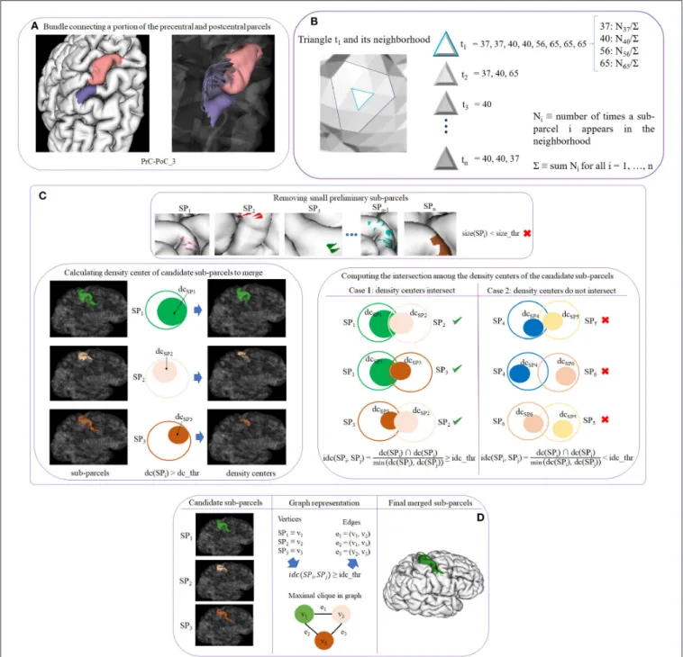
2.2.6.1. Sub-step 5.1: creating preliminary sub-parcels
This sub-step creates preliminary sub-parcels based on the fiber bundle intersection information of each triangle. Each bundle in the atlas will define two preliminary sub-parcels, corresponding to the two extremities of the bundle. Sub-parcel names were defined following the bundle names. A label is also internally associated to identify each sub-parcel. Figure 3A shows an example of the two preliminary sub-parcels created for bundle PrC-PoC_3 of a subject. Each anatomical parcel, given by the Desikan-Killiany atlas, is formed by several preliminary sub-parcels, which overlap each other, representing all the bundles that connect the region.
2.2.6.2. Sub-step 5.2: calculating probability maps
This sub-step computes the probability of each sub-parcel in each triangle across the subjects. With this information, the probability maps for all the sub-parcels over the mesh are inferred, and the most probable sub-parcels for each triangle are also obtained. Let us denote ti with i = 1, . . . , n a triangle of the mesh, and
consider the neighborhood of tias all the triangles that share a
vertex or and edge with ti. For each triangle, we count the number
of times a sub-parcel appears in the neighborhood Ni, with i =
1, . . . , n. To achieve this, for each triangle ti, a list is created
with the labels of the sub-parcels that intersect the triangle or its neighborhood. A label is added for each bundle fiber intersection, for each subject. Figure 3B shows an example for a triangle t1and
its neighborhood. For instance, t1has associated the list of
sub-parcel labels that intersect the triangle and its neighbor triangles, for all the subjects. Each label has also associated the number of times the sub-parcel appears in the neighborhood (Ni). We also
calculate 6 equal to the sum of all the counts Ni. To obtain the
probability of each label in each triangle, the value Niis divided
by 6. Finally, for each triangle, the list of probabilities is sorted in descending order.
2.2.6.3. Sub-step 5.3: processing preliminary sub-parcels
The purpose of this step is to solve the overlap that exists between the preliminary sub-parcels within each anatomical parcel of the cortex.
First, small preliminary sub-parcels are eliminated. We denote a preliminary sub-parcel as SPi, with i = 1, . . . , n as the label of
the sub-parcel, and size_thr as the threshold used to eliminate the smaller sub-parcels. The size is measured in terms of the number of triangles of the sub-parcel, as the areas of the mesh triangle are very homogeneous. The criterion of elimination size_thr is defined in terms of the percentage of triangles of the sub-parcel with respect to the corresponding anatomical region. After this processing, a set of candidate sub-parcels is obtained and the probability maps are recalculated according to the reduced set of sub-parcels (see Figure 3C top image).
The sub-parcels are highly overlapped, but if we look at their intersection density, we can observe that the overlapping can occur in regions with low density, or in a region of high density for one parcel, but a region of low density for another sub-parcel. Indeed, the fiber intersection density is not homogeneous across the mesh surface for most of the sub-parcels. In fact, in most of the cases, only a portion of the sub-parcels present a high density. Since a merging of the sub-parcels is required to obtain a hard parcellation, we calculate the density center of each sub-parcel to perform a better analysis. The density center is defined as the area where the highest concentration of fibers exists for each triangle. We denote the sub-parcel as SPi with
i = 1, . . . , n as the label of each sub-parcel, and the density center as dc(SPi). Each triangle of a sub-parcel has associated a list with
the probability of each sub-parcel present in the triangle. The density centers are then defined using a minimum probability threshold of dc_thr (density center threshold) for dc(SPi). A
parcel can have several density centers spread over the sub-parcel. Some examples of parcel density centers are shown in Figure 3C bottom left image. The left column displays three sub-parcels corresponding to the precentral anatomical parcel. In the middle column, we represent each sub-parcel SPi as a
circle of the same color and mark each density center with another filled circle inside. The third column shows the regions for dc(SPi) > dc_thr, corresponding to the density center of
each sub-parcel.
Once the density centers have been calculated, we compute the intersection among them, for the candidate sub-parcels. The objective is to check if there is a significant overlap between the candidate sub-parcels, to merge them. Given all the pairs of sub-parcels, we denote the density center of the first sub-parcel as dc(SPi) and the second sub-parcel as dc(SPj), i and j being
the labels of each sub-parcel, with i, j = 1, . . . , n and i <> j. The intersection between each sub-parcel pair is calculated based on the intersection of their density centers (triangles), following equation 1:
idc(SPi, SPj) =
dc(SPi) ∩ dc(SPj)
min(dc(SPi), dc(SPj))
(1) To define a significant intersection, we use a threshold idc_thr (intersection of density centers threshold), where idc ≥ idc_thr
FIGURE 3 | Schematics of cortex parcellation (STEP 5) sub-steps. (A) Sub-step 5.1: creating preliminary sub-parcels. Preliminary sub-parcels are created based on the fiber bundle intersection and the labels of each triangle. (B) Sub-step 5.2: calculating probability maps. The probability of each sub-parcel label in each triangle across the subjects is calculated. (C) Sub-step 5.3: processing preliminary sub-parcels. This step deals with the preliminary sub-parcel overlapping. First, sub-parcels that do not exceed a size threshold (size_thr) are eliminated (top image). Next, the density center (dc) for each sub-parcel is calculated. Preliminary sub-parcels with a dcgreater than a threshold (dc_thr) become potential candidates to merge (bottom left image). The intersection (idc) of each pair of dc is calculated (bottom right image). (D) Sub-step 5.4: merging of candidate sub-parcels. In order to merge the most overlapped sub-parcels, the problem is represented by a graph, where the candidate sub-parcels are the vertices, and edges are added for the pairs of candidate sub-parcels with a high overlapping. Finally, maximal cliques are used to select the group of sub-parcels to be merged.
will define the sub-parcels that are candidates to merge. Figure 3C bottom right image, illustrates an example of sub-parcel intersection analysis. The first column shows a case where three sub-parcels intersect between them, considering
the intersection of the three pairs of sub-parcels. The second column shows the opposite case, where no important overlaps between the sub-parcels exist, and are therefore not considered as candidates to merge. Once all the candidate sub-parcels have
been obtained, the next processing step performs the merging of them.
2.2.6.4. Sub-step 5.4: merging of candidate sub-parcels
In this step, the overlap between sub-parcels is analyzed using a graph representation of the sub-parcels and their intersection, to merge the parcels that are significantly intersected with each other. More specifically, the objective is to find the groups of sub-parcels that are all intersected with each other within each group. This problem can be solved using a graph representation of the sub-parcel intersections and a maximal clique algorithm.
Let G = (V, E) be an undirected graph, where each vertex v ∈ V represents a candidate sub-parcel. For each candidate sub-parcel pair v1and v2in G, we create an edge between them
e = (v1, v2) ∈ E if the probability that the intersection of
the density centers, idc(SPi, SPj) (Equation 1) is superior to the
threshold idc_thr. The graph will therefore contain only the relevant intersections between sub-parcels, i. e., where the density centers present a minimum percentage of overlapping. Once G is created, the idea is to obtain the vertices in the graph that are all connected with each other. Therefore, we use the graph algorithm called clique (Karp, 1972) that aims to find subsets of vertices that are adjacent (connected), and merge them in a single sub-parcel. We use a clique variant called maximal clique, which finds a clique with the largest possible number of vertices. The problem of finding maximal cliques is that it is computationally expensive (NP-hard) (Woeginger, 2003; Sipser, 2006), however, for sparse graphs the complexity is less (Eppstein and Strash, 2011). After having calculated all the maximal cliques that are in G, these are sorted by size (number of vertices), in descending order. Following this order, the candidate sub-parcels of each maximal clique are merged to obtain the biggest number of fusions. This processing leads to the final sub-parcels, composed of merged candidate sub-parcels, candidate sub-parcels that were not merged, and the sub-parcels that were not candidates to merge (not included in the graph).
Figure 3Dshows an example of merging for three candidate sub-parcels of the precentral anatomical parcel. In the first column, the candidate sub-parcels, denoted by SPi, are displayed.
In the second column, a graph representation of the intersections is included, in which each sub-parcel SPiis a vertex vi. If the idc
(see Equation 1) between a pair of sub-parcels is superior to the threshold idc_thr, an edge is created between both vertices. The graph G and the maximal clique are also graphically represented. The third column shows the final sub-parcel, resulting from the merging of the three sub-parcels.
Finally, the probability maps for each triangle are recalculated. The most probable label is also determined, with the purpose of obtaining a hard parcellation (see Figure 1F).
2.2.7. Step 6: Sub-Parcel Post-processing
The last step of the parcellation method deals with post-processing sub-parcels, to better define the final sub-parcels and the hard parcellation. It receives as an input the mesh vertex labels of the parcel subdivision from the previous step. The post-processing is composed of three morphological operations performed over the cortical mesh.
2.2.7.1. Removing small connected components
The sub-parcels obtained in the previous step may be formed by more than one connected component. Some small components are in fact groups of a few triangles isolated from the main component. These small components are therefore removed using a graph representation of each sub-parcel. The connected components of a graph can be easily calculated (Tarjan, 1972), and then ordered by size in descending order. Next, the largest connected component is kept. For each small connected component, the second most probable label in the list containing the probability map of the corresponding triangles is selected. The neighborhood of each connected component is then analyzed to verify if a match between the second label of the triangle and its neighborhood exists. In most cases this value is appropriate, but if this is not the case, the label is removed. Figure S5 shows an example of this processing for the supramarginal (SM) parcel, with three sub-parcels.
2.2.7.2. Sub-parcel opening
For each sub-parcel, the morphological operation called opening (Heijmans, 1994) is applied over the mesh, in order to eliminate isolated triangles that are scattered throughout the mesh. This operation is the result of the application of erosion + dilation operations. These two operations were therefore sequentially applied.
Figure S6shows an example of the results after applying the post-processing, with size_thr = 0.1, dc_thr = 0.1, and idc_thr = 0.1. This hard parcellation or parcellation result, consists of 85 sub-parcels in the left hemisphere and 72 sub-parcels in the right hemisphere.
2.3. Parcellation Method Parameter
Settings
This section provides the parcellation method configuration parameters. The parcellation method has three configurable parameters for generating a hard parcellation: size_thr, dc_thr and idc_thr. Note that all the parameters are adapted to the anatomical region and sub-parcel size, and are defined as percentages.
2.3.1. Minimum Preliminary Sub-Parcel Size Threshold (size_thr)
This parameter is used to eliminate small preliminary sub-parcels that do not exceed a certain size, concerning the average size of the sub-parcels of an anatomical parcel. We visually evaluated the results with different values of size_thr, between 0.05 and 0.40. Big values, >0.25, eliminate big preliminary sub-parcels, and therefore, leave some regions in the cortex uncovered. On the other hand, values inferior to 0.1 remove only very small preliminary sub-parcels. We therefore selected a conservative value of size_thr = 0.10, which will only eliminate small sub-parcels, with a size inferior to the 10% of the average sub-parcel size on a region.
Figure S4shows an example of Removing of small preliminary sub-parcels sub-step, belonging to Step 5 of the parcellation method for the precentral anatomical parcel (PrC), using size_thr = 0.10 and size_thr = 0.30.
2.3.2. Preliminary Sub-Parcel Density Center Threshold (dc_thr)
This parameter determines the size of the density center (dc) of a preliminary sub-parcel. It defines the minimum percentage of probability of the sub-parcel in a triangle used to consider the triangle as part of the density center, and can potentially be considered for the intersection analysis. We varied its value between 0.10 and 0.30. The higher the chosen value, the smaller the density centers are, and the fewer intersections will be found when determining the intersection of the sub-parcels.
2.3.3. Intersection of Density Centers Threshold (idc_thr)
This parameter defines the minimum intersection between the density centers of two sub-parcels to be considered as overlapped, and therefore, candidates to merge. This parameter is varied from 0.10 to 0.40. The lower the idc_thr, the more likely it is that the sub-parcels will merge.
3. RESULTS
We implemented Steps 2 and 4 in C++11, which are also parallelized with OpenMP. The rest of the steps were performed in the Python programming language version 3.6. We executed our experiments on a computer with a 12-core Intel Core i7-8700K CPU 3.70GHz, 12MB of shared L3 cache, and 32GB of RAM, using Ubuntu 18.04.2 LTS with kernel 4.15.0-51 (64 bits). For the tests, we used the tractography datasets of the 79 subjects of the ARCHI database. We used the same database for the atlas creation and the parcellation creation to guarantee the best results. The methods are publicly available at https://github.com/ andvazva/Parcellation.
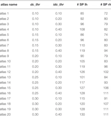
Table 1 shows 20 parcellations (atlases) generated with the proposed method, resulting from different sets of parameters, with varying density center thresholds (dc_thr = 0.10, 0.15, 0.20, 0.25, 0.30) and intersection of density center thresholds (idc_thr = 0.10, 0.20, 0.30, 0.40), and a fixed value of size_thr = 0.10. The atlases are identified by a number. The table also lists the number of sub-parcels in the left hemisphere (# SP lh) and right hemisphere (# SP rh) obtained for each atlas. As dc_thr and idc_thr increase, the number of sub-parcels in both hemispheres increase, as more restrictive values are used to define a significant sub-parcel intersection, leading to an inferior number of merges.
A first observation is the asymmetry in the number of sub-parcels between both hemispheres, with more sub-sub-parcels in the left hemisphere for all the parcellations. A similar result was found in the parcellation created byLefranc et al. (2016), based on the same database, with 126 parcels for the left hemisphere and 113 parcels for the right hemisphere. This could be due to a higher variability found in the number of fibers across subjects in the left hemisphere. To gain insight on how much variability there is with respect to the population average, we calculated the coefficient of variation (CV) of the number of fibers in both hemispheres across subjects. CV measures the ratio between the standard deviation (σ ) and the mean (µ), i. e. CV = σ/µ. The resulting CV for the left hemisphere is 0.23, while it is 0.21
TABLE 1 | Parameters used and the number of sub-parcels obtained per hemisphere for each configuration of parameters for the cortex parcellation method.
atlas name dc_thr idc_thr # SP lh # SP rh
atlas 1 0.10 0.10 85 72 atlas 2 0.10 0.20 92 80 atlas 3 0.10 0.30 96 79 atlas 4 0.10 0.40 108 82 atlas 5 0.15 0.10 86 74 atlas 6 0.15 0.20 96 80 atlas 7 0.15 0.30 110 83 atlas 8 0.15 0.40 119 94 atlas 9 0.20 0.10 90 79 atlas 10 0.20 0.20 105 83 atlas 11 0.20 0.30 119 96 atlas 12 0.20 0.40 126 102 atlas 13 0.25 0.10 101 84 atlas 14 0.25 0.20 117 93 atlas 15 0.25 0.30 127 106 atlas 16 0.25 0.40 128 111 atlas 17 0.30 0.10 115 91 atlas 18 0.30 0.20 120 107 atlas 19 0.30 0.30 128 111 atlas 20 0.30 0.40 130 111
The first column shows the name given to each atlas (parcellation result), based on a correlative number. The second and third columns list the different values for the density center (dc_thr) and the intersection of the density center (idc_thr) thresholds, for each generated atlas. Columns four and five list the number of sub-parcels obtained for the left (#SP lh) and right (# SP rh) hemispheres, respectively.
for the right hemisphere. One possible cause of the asymmetry in the number of sub-parcels may be that the higher variability in the number of fibers in the left hemisphere could produce a higher variability of connections in the cortex, resulting in smaller parcels.
In the following subsections, we first perform a reproducibility analysis of the connectivity for the generated parcellations across subjects. A comparison of the generated atlases is then performed based on the similarity of their sub-parcels. Finally, a comparison is carried out with some state-of-the-art parcellations based on different modalities.
3.1. Reproducibility Analysis
To test the consistency of the generated parcellations across the subjects, a reproducibility analysis was performed (Arslan et al., 2018). For this purpose, for each subject, its tractography is taken and intersected with its mesh by means of the obtained parcellation. Afterwards, a binary connectivity matrix of size n ∗ n is created, where n is the total number of sub-parcels belonging to the resulting parcellation. If there is a connection between two sub-parcels, it is indicated with a one, otherwise it is indicated with a zero. This procedure is shown in Figure 4. Finally, the Dice coefficient (Duda et al., 2014) is used to measure the similarity of the binary connectivity matrices across subjects for each obtained parcellation.
FIGURE 4 | Brain connectivity analysis. First, the tractography of each subject is intersected with the subject’s cortical mesh, using the generated cortical parcellation. Then, a square connectivity matrix n ∗ n is created, where n is the total number of sub-parcels in the parcellation. The matrix contains a 1 where there exists a connection between the pair of corresponding sub-parcels and zero in other case.
The Dice coefficient measures the similarity between two sets (Equation 2).
DSC = 2|A ∩ B|
|A| + |B| (2)
where |A| and |B| are the number of elements of sets A and B, respectively, and DSC is the Dice coefficient. DSC ranges between 0 and 1; the closer to 1, the greater the similarity between the two sets.
To compute the Dice coefficient between two connectivity matrices, the bctpy Python library (https://github.com/aestrivex/ bctpy) was used, which is an adaptation of the Matlab Brain Connectivity Toolbox for Python (Rubinov and Sporns, 2010). For each generated parcellation, DSC was calculated between the connectivity matrices of each pair of subjects and was then averaged (see Figure 5). A cross-validation analysis was also performed and is included in section 1.7 of the Supplementary File.
The results show that there is no great variability between the generated atlases in terms of the similarity between the connectivity matrices obtained for the different subjects. In general, the similarity decreases with the number of sub-parcels, which is expected due to the relatively bigger effect of noise and inter-subject variability, but is still good for a high number of parcels. The atlases with the least number of sub-parcels therefore have the highest similarity between the subjects, which are atlas 1 and atlas 5.
Additionally, we performed some tests based on a network analysis (Bullmore and Sporns, 2009; Cohen and D’Esposito,
FIGURE 5 | Average Dice coefficient for each parcellation (atlas) configuration, given by Table 1. The Dice coefficient was calculated between the
connectivity matrices of each pair of subjects and then averaged. The results show a slight variability between the generated atlases. Due to the
inter-subject variability, the similarity is smaller with a larger number of parcels.
2016), provided in the Supplementary File. Section 1.5 describes the graph construction, while section 1.6 contains the network metrics calculation. These metrics are highly sensitive to the number of sub-parcels. For example, the results show a better small-world ω coefficient for atlas 1 and atlas 5. We selected the atlas 5 as a candidate for comparison with other state-of-the-art
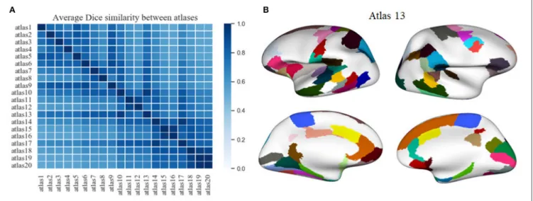
FIGURE 6 | A comparison between the twenty atlases generated with the proposed method, based on different sets of the three parameters of the method. (A) Matrix obtained from the pairwise comparison of the sub-parcels of the different atlases, based on the average Dice coefficient (the closer to one, the more similar). The atlas most similar to the other atlases, i. e., the atlas with the higher mean Dice coefficient, is atlas 13. (B) A visualization of the sub-parcels of atlas 13 that are in common with all the other parcellations, based on a Dice coefficient ≥0.6. The first column shows the left hemisphere with 47 sub-parcels in common, while the second column illustrates the 41 sub-parcels in common for the right hemisphere.
methods, due to its high reproducibility, and as an example of an atlas with a small number of sub-parcels.
We applied another criterion to select a parcellation, based on the atlas that is most similar to the remaining generated atlases. This atlas is in some way the most homogeneous atlas among all the atlases generated by the parcellation method. To select the atlas, we compared between them, all the sub-parcels from the 20 generated atlases, through the construction of a similarity matrix. For each pair of atlases, we used the Dice coefficient to compare all the sub-parcels between the two atlases. To obtain the final result between two atlases, the Dice coefficient of all sub-parcels was averaged, representing the degree of similarity between the two atlases. The closer the coefficient is to one, the more similar the two atlases are. Figure 6A illustrates the similarity matrix for the 20 atlases. Finally, we selected the most reproducible atlas among the atlases, which presented the highest Dice coefficient on average, resulting in the atlas 13. Table S4 illustrates the number of sub-parcels per hemisphere in atlas 5 and atlas 13. Table S5 shows a detailed description of the number of sub-parcels per hemisphere that have the generated atlases in common. Furthermore, Figure 6B illustrates the sub-parcels that atlas 13 has in common with the others atlases, based on a Dice coefficient ≥0.6 (47 sub-parcels in the left hemisphere and 41 sub-sub-parcels in the right hemisphere).
As mentioned above, we selected atlas 5 for comparisons with state-of-the-art atlases because it is an example of an atlas with a low number of sub-parcels, and has high reproducibility. On the other hand, atlas 13 was selected as the most similar atlas to the remaining generated atlases. Atlas 5 contains 160 sub-parcels, while atlas 13 contains 185 sub-parcels. Table S4 lists the differences between atlas 5 and atlas 13 in terms of the number of sub-parcels per each DK atlas region. About 70% of
FIGURE 7 | Example of two sub-parcels of atlas 13 with biological relevance. These sub-parcels follow the most common definitions of the Broca’s (Amunts and Zilles, 2012) (in red) and Wernicke’s (Geschwind, 1970) (in green) areas, related to language processing. Also, the fibers connecting these sub-parcels are illustrated in blue, which correspond to the arcuate fasciculus (Catani and Mesulam, 2008).
the sub-parcels are similar. The differences, in general, refer to a subdivision of the sub-parcels.
Finally, we show an example to illustrate the biological significance of a pair of sub-parcels obtained by our parcellations. We selected the sub-parcels of atlas 13 that better match the most common definitions of Broca’s (Amunts and Zilles, 2012) and Wernicke’s (Geschwind, 1970) areas, related to language processing. As illustrated in Figure 7, these regions seem to correspond to the Broca’s (in red) and Wernicke’s (in green) areas. Moreover, we illustrate the fibers connecting both sub-parcels, which correspond to the arcuate fasciculus, in agreement with
the literature (Catani and Mesulam, 2008). In fact, this fascicle is present in the fused bundle atlas used to create the parcellations, and the segmentation of this bundle is very stable across subjects. Its connections therefore define the described sub-parcels also present in atlas 5. Further studies are required to validate, in detail, the biological significance of diffusion-based parcellations.
3.2. Comparison With State-of-the-Art
Parcellations
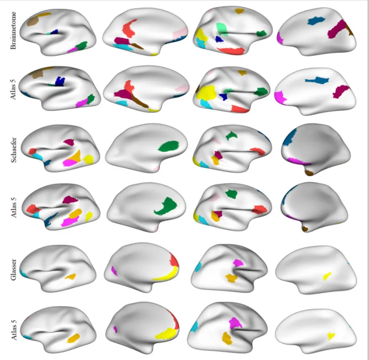
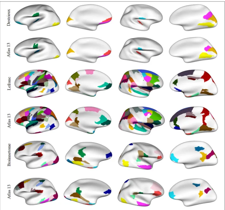
This section provides a comparison between atlas 5 and atlas 13, generated by our parcellation, with other state-of-the-art parcellations based on different modalities. For the comparisons we used Destrieux atlas (Destrieux et al., 2010), based on macro anatomy with 150 parcels, and Lefranc parcellation (Lefranc et al., 2016), based on dMRI, containing 239 parcels. Based on a multimodal approach, we used the Brainnetome atlas (Fan et al., 2016), which is composed of 210 cortical parcels and 36 sub-cortical parcels and Glasser’s atlas (Glasser et al., 2016), which contains 360 parcels, 180 per hemisphere. In addition, based on functional MRI, we used the PrAGMATiC atlas (Huth et al., 2016), which has 320 parcels, Schaefer’s atlases (Schaefer et al., 2017), consisting of several parcellations varying from 100 to 1,000 parcels, and Yeo’s atlas (Yeo et al., 2011), which is formed by seven or 17 networks. All the atlases are in MNI space, and are available in image format, with the exception of Lefranc which is available as a labeled mesh.
To be able to compare the parcellations in image format with our atlases, we first performed a mapping of the atlases to a cortical mesh. For each atlas, we labeled a cortical mesh in MNI space, by assigning the label of the closest voxel in the image atlas, to each mesh vertex. We then compared our atlases with the other parcellations, by evaluating the similarity of each sub-parcel of atlas 5 and atlas 13 with each parcel of the other atlases, using the Dice coefficient over the mesh triangle labels. In this case, Dice’s coefficient will evaluate the degree of overlap between a pair of parcels, ranging from 0, for a total dissimilarity, to 1, for a complete similarity. Moreover, to identify the sub-parcels in atlas 5 and atlas 13, we named them based on the anatomical regions connected by these sub-parcels, based on Desikan-Killiany atlas. For example, the parcel lh_RMF-CMF-SF_0 connects RMF with CMF and SF regions. The number (_0) denotes the index of the sub-parcel, which depends on the number of sub-parcels in an atlas with the same connections. Prefixes lh or rh refer to the left or right hemisphere. For more details, Table S3 lists the names of anatomical regions of the Desikan-Killiany atlas. To perform the tests, both atlases, atlas 5 and atlas 13, were applied to one subject in MNI space as a representative subject (Subject 001 from the ARCHI database). The same subject was used for all tests. Any other subject transformed to MNI space could be used, because there is a correspondence between the mesh triangles of all the subjects, which have the same triangle indexes.
Tables 2, 3 contain the results of the comparison between atlas 5 and atlas 13 with the other atlases. For each state-of-the-art parcellation, the total number of parcels or networks that it contains, as well as the number of parcels similar to atlas 5 and atlas 13, between different ranges of Dice coefficient, are
indicated. In the table, the minimum Dice value considered is 0.5, while similarity values superior to 0.9 were not found.
The Destrieux atlas was generated using 12 datasets and algorithms that classified each vertex in a computer-assisted manual manner and divided the cerebral cortex into 75 parcels per hemisphere, giving a total of 150 parcels. The comparison of Destrieux and atlas 5, obtained 37 similar parcels with Dice ≥0.5 in the two hemispheres. The most similar parcel is in the right hemisphere, corresponding to G_cuneus, located in the occipital lobe (cuneus) and corresponding to rh_Cu-Li-MOF_0 of atlas 5. In the left hemisphere we have the parcels S_suborbital and G&S_subcentral corresponding to the frontal (suborbital sulcus) and parietal (subcentral gyrus) lobes. In atlas 5 these parcels correspond to the sub-parcels lh_MOF-LOF-LO_0 and PoC-Ins-SM_0, respectively. The comparison between Destrieux and atlas 13 obtained 45 similar parcels with Dice ≥0.5 between both hemispheres. We highlight from the left hemisphere, the parcel S_suborbital of Destrieux, which has its equivalent in atlas 13 of the sub-parcel lh_MOF-IC-PrCu_0, located in the frontal lobe (suborbital sulcus). In the right hemisphere, the parcels G_cuneus and G&S_subcentral of Destrieux are similar to the sub-parcels rh_Cu-Li_0 and rh_PoC-SM_0 of atlas 13, and are located in the occipital (cuneus) and parietal (subcentral gyrus) lobes, respectively.
With respect to the comparison with Lefranc, this parcellation has our method in common, which was based on the same database (ARCHI) and uses the regions of Desikan-Killiany atlas as an input. Furthermore, the method uses the whole dMRI tractography as an input. The Lefranc algorithm compresses the connectivity profiles of each gyrus, taking into account the inter-subject variability, and considering inter-inter-subject high-density connectivity areas extracted using a surface-based watershed algorithm. Finally, it applies a clustering algorithm over the reduced connectivity profiles to obtain a group-wise parcellation, which consists of 239 parcels (126 in the left hemisphere and 113 in the right hemisphere). In the comparison made between Lefranc and atlas 5, we found 121 similar parcels with Dice ≥0.5. The most relevant parcel in the left hemisphere is lh.caudalmiddlefrontal.1 which corresponds to the CMF-PrC-RMF_1 sub-parcel in atlas 5, located in the frontal lobe (caudal middle frontal gyrus). The most similar parcels in the right hemisphere are rh.inferiorparietal.3 and rh.precuneus.2, both belonging to the parietal lobe, specifically, the inferior parietal cortex and precuneus cortex. They correspond to the sub-parcels IP-IT-MT_0 and PrCu-CAC-PoCi-SF_0 in atlas 5, respectively. Lefranc and atlas 13 have 130 parcels in common. The most similar parcels in the left hemisphere are lh.supramarginal.2 and lh.postcentral.3. Both parcels are located in the parietal lobe, namely in the supramarginal and post-central gyri. The equivalent sub-parcels in atlas 13 are lh_SM-PrC_0 and lh_PoC-Ins-SM_0. In the right hemisphere, we found rh.inferiorparietal.2 parcel, which is located in the parietal lobe (inferior parietal cortex) and is similar to sub-parcel rh_IP-SM-PrC_0 in atlas 13.
The Brainnetome atlas relies on a multimodal approach. Multimodal information consists of diffusion MRI, functional MRI, and structural MRI data. This parcellation was based on
TABLE 2 | Number of similar parcels found between atlas 5 and parcellations based on different MRI modalities.
Parcellation name ≥0.5 and <0.6 ≥0.6 and <0.7 ≥0.7 and <0.8 ≥0.8 and <0.9
Brainnetome (210 parcels) 37 parcels 21 parcels 4 parcels 0 parcels
Destrieux (150 parcels) 26 parcels 8 parcels 2 parcels 1 parcel
Glasser (360 parcels) 31 parcels 7 parcels 2 parcels 0 parcels
Lefranc (239 parcels) 47 parcels 32 parcels 26 parcels 16 parcels
PrAGMATiC (320 parcels) 33 parcels 13 parcels 2 parcels 0 parcels
Schaefer (100 parcels) 26 parcels 9 parcels 2 parcels 0 parcels
Schaefer (200 parcels) 37 parcels 15 parcels 4 parcels 0 parcels
Yeo (7 networks) 0 parcels 0 parcels 0 parcels 0 parcels
Yeo (17 networks) 4 parcels 0 parcels 1 parcel 0 parcels
For each parcellation, the total number of parcels or networks that compose it is listed, as well as the number of similar parcels based on Dice’s coefficient. This coefficient ranges from 0 to 1, with 1 being total similarity. The number of similar parcels is divided into four groups, according to Dice’s coefficient value.
TABLE 3 | Amount of parcels in common between atlas 13 and other parcellations based on the Dice coefficient.
Parcellation name ≥0.5 and <0.6 ≥0.6 and <0.7 ≥0.7 and <0.8 ≥0.8 and <0.9
Brainnetome (210 parcels) 40 parcels 26 parcels 5 parcels 0 parcels
Destrieux (150 parcels) 33 parcels 8 parcels 4 parcels 0 parcels
Glasser (360 parcels) 40 parcels 14 parcels 0 parcels 0 parcels
Lefranc (239 parcels) 55 parcels 35 parcels 27 parcels 13 parcels
PrAGMATiC (320 parcels) 43 parcels 19 parcels 3 parcels 0 parcels
Schaefer (100 parcels) 24 parcels 10 parcels 2 parcels 0 parcels
Schaefer (200 parcels) 31 parcels 22 parcels 4 parcels 0 parcels
Yeo (7 networks) 0 parcels 0 parcels 0 parcels 0 parcels
Yeo (17 networks) 4 parcels 0 parcels 0 parcels 0 parcels
The first column lists the names for each parcellation and the number of parcels or networks that compose them. The other columns detail the total number of parcels in common for each Dice interval. This coefficient ranges between 0 and 1, being 1 the biggest similarity achieved.
80 subjects of the Human Connectome Project (HCP) database and contains 210 cortical parcels (105 per hemisphere) and 36 subcortical parcels. This atlas has atlas 5 and atlas 13 which uses dMRI, in common, but employs probabilistic rather than deterministic tractography. Furthermore, both methods use the Desikan-Killiany atlas as input information. Atlas 5 and Brainnetome have 62 parcels in common. We can highlight parcel A9_46d_L (left hemisphere) located in the frontal lobe (middle frontal gyrus), which is linked to the atlas 5 sub-parcel called lh_RMF-CMF-SF_0, and is related to inhibition, social cognition, and word generation. In the right hemisphere, parcel msOccG_R of Brainnetome, located in the occipital lobe (lateral occipital cortex), is similar to sub-parcel rh_SP-LO-MT_0 of atlas 5, which is related to spatial ability, shape vision, motion vision, and inhibition. We also have parcel A23c_R which is similar to sub-parcel rh_PoCi-CAC-PrCu-RAC_0, located in the limbic lobe (cingulate gyrus), and which is related to emotions, reward, and pain. Moreover, atlas 13 and Brainnetome have 71 parcels in common. The three most similar parcels correspond to the left hemisphere. Brainnetome parcel A9_46d_L corresponds in atlas 13 to the sub-parcel lh_RMF-CMF-SF_0 (middle frontal gyrus) and is related to inhibition, social cognition, and word generation. Parcel A40rv_L is linked to sub-parcel lh_SM-PrC_0 in atlas 13 and is located in the parietal lobe (inferior parietal)
and has functions related to audition, pain, grasping, and discrimination. Finally, parcel A8dl_L corresponds to sub-parcel lh_CMF-Op_0 of atlas 13, is located in the frontal lobe (superior frontal gyrus), and is related to emotion, cognition, and memory. Glasser atlas is also based on a multimodal approach. This parcellation is based on functional connectivity (resting state), microstructural architecture, functional specialization (task-fMRI), and topography information. In addition, it uses data from 449 subjects of the HCP database and generates a final parcellation which consists of 360 parcels (180 per hemisphere). We found 40 parcels in common with atlas 5. In the left hemisphere, sub-parcel lh_Or-LOF-Ins-LO_0 of atlas 5 corresponds to parcel L_a47r_ROI located in the frontal lobe (Orbital and Polar Frontal Cortex) of Glasser and is linked to relational-match, gambling, working memory, language (story and math), and face-shape recognition. Continuing in the same hemisphere, another relevant Glasser parcel is L_POS1_ROI, located in the parietal lobe (Posterior Cingulate Cortex), which is similar to sub-parcel lh_PrCu-PH-En_0 and is related to language (story and math) and scene selection. As for the right hemisphere, the R_V3A_ROI parcel which is located in the occipital lobe (Dorsal Stream Visual Cortex) is equivalent to the rh_SP-LO-MT_0 sub-parcel of atlas 5, which is related to retinotopic areas, gambling, and emotion. The The comparison between