Champagne: UQÀM and CIRPÉE
champagne.julien@uqam.ca
Kurmann: UQÀM and CIRPÉE
kurmann.andre@gmail.com
We thank John Schmitt, Jean Roth and Barry Hirsch for help with the CPS data; Wayne Gray and Daniel Parent for making available their datasets; and François Gourio and Urban Jermann for comments. Earlier versions of this paper have been presented at the 2009 conference of the Société Canadienne de Science Économique, the 2009 SCBR Conference, and the Wharton macro lunch. Financial support from the SSHRC and the hospitality of the Wharton School at the University of Pennsylvania, where part of this project was completed, is gratefully acknowledged.
Cahier de recherche/Working Paper 10-10
The Great Increase in Relative Volatility of Real Wages in the United
States
Julien Champagne André Kurmann
Abstract:
This paper documents that over the past 25 years, aggregate hourly real wages in the United States have become substantially more volatile relative to output. We use micro-data from the Current Population Survey (CPS) to show that this increase in relative volatility is predominantly due to increases in the relative volatility of hourly wages across different groups of workers. Compositional changes, by contrast, account for at most 12% of the increase in relative wage volatility. Using a Dynamic Stochastic General Equilibrium (DSGE) model, we show that the observed increase in relative wage volatility is unlikely to come from changes outside of the labor market (e.g. smaller exogenous shocks or more aggressive monetary policy). By contrast, increased flexibility in wage setting is capable of accounting for a large fraction of the observed increase in relative wage volatility. At the same time, increased wage flexibility generates a substantial decrease in the magnitude of business cycle fluctuations, which suggests a promising new explanation for the Great Moderation.
Keywords: Wage volatility, business cycles, great moderation, current population
survey, dynamic stochastic general equilibrium models
1
Introduction
The 25 years prior to the current recession were a time of unprecedented macroeconomic stability for the United States. During that period, referred to by many as the ’Great Moderation’, the business cycle volatility of U.S. output declined by more than 50% and the volatility of many other
macroeconomic aggregates fell by similar proportions.1
In this paper, we show that the Great Moderation does not apply to one of the most prominent labor market aggregates: the average real hourly wage (or ’aggregate wages’for short). Speci…cally, we document the following results:
1. From 1948-1984 to 1984-2006, the business cycle volatility of the aggregate wage increased between 30 and 70 percent, depending on the …ltering method and nominal de‡ator used. 2. As a result, the business cycle volatility of the aggregate wage relative to the volatility of
aggregate output experienced a three- to four-fold increase over the two sample periods. The increase in both absolute and relative volatility of aggregate wages raises several questions. First, to what extent does this increase apply to di¤erent groups of workers? Second and related, how much of the increase in volatility is due to compositional changes of the workforce; i.e. a shift of the workforce towards jobs with more volatile wages? Third, to what extent is the increase in volatility related to structural changes in the U.S. labor market? Fourth, how do such labor market changes contribute to our understanding of business cycle ‡uctuations in general and the Great Moderation in particular?
To answer the …rst and second question, we use microdata from the Current Population Survey (CPS) to construct hourly wage series for di¤erent groups of workers. We document that the increase in absolute volatility of the real wage is not generalized but concentrated among male, skilled and young workers. Also, there are large di¤erences across industries, with absolute volatilities of hourly wages in many industries decreasing. However, these decreases are generally modest and thus, the volatility of real hourly wages relative to the volatility of aggregate output increases substantially across most of decompositions considered. We call this phenomenon the ’Great Increase in Relative Volatility of Real Wages’.
To quantify how much of the increase in the relative volatility of aggregate wages is due to increases in relative volatility of wages across di¤erent groups of workers, we develop an accounting method that allows us to decompose the increase in aggregate wage volatility into compositional changes and changes in relative volatilities and correlations. The main result coming out of this
exercise is that the large increase in relative volatility of aggregate wages is predominantly due to the increase in the relative volatility of wages of the di¤erent worker groups. Compositional changes of the labor force, by contrast, account for at most 12% of the increase in the relative volatility of the aggregate wage. This suggests that the increase in the relative volatility of aggregate wages is due to changes in the economic environment that a¤ected wage dynamics of most groups of workers, although to varying degrees.
To address the third and fourth question, we build a small Dynamic Stochastic General Equilib-rium (DSGE) model with a stylized wage setting function that allows for varying degrees of wage rigidity. We calibrate the model consistent with U.S. data and show that while changes in the importance of exogenous shock processes can have a sizable e¤ect on the absolute volatility and cyclicality of aggregate wages, their e¤ect on the relative volatility of wages is negligible. Similarly, structural changes to the economy that do not directly a¤ect the labor market (e.g. a more ag-gressive monetary policy response to in‡ation) are unlikely to have a large e¤ect on the relative volatility of wages. By contrast, more ‡exible wage setting is capable of accounting for a large fraction of the observed increase in relative wage volatility and simultaneously implies a substantial
decrease in the magnitude of business cycle ‡uctuations for given exogenous shocks.2 We con…rm
the robustness of our …ndings in the larger DSGE model of Smets and Wouters (2007) that contains many frictions and shocks. These results suggest that the hypothesis of increased wage ‡exibility has a lot of potential to rationalize the observed changes in U.S. labor market dynamics and at the same time provides a promising new explanation for the Great Moderation.
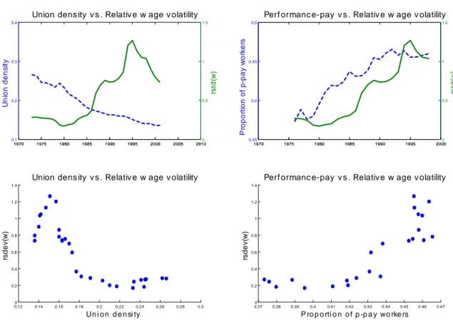
The hypothesis of increased ‡exibility in wage setting is appealing for several reasons. On the one hand, it is consistent with the documented rise in individual earnings volatility in the U.S. in the 1980s and 1990s (e.g. Gottschalk and Mo¢ tt, 1994; Dynan et al., 2008). On the other hand, the U.S. labor market has undergone several important changes over the past 25 years that are likely to have led to increased ‡exibility in wage setting. Among them are the large decrease in private sector unionization (e.g. Farber and Western, 2001); the shift towards performance-pay contracts (e.g. Lemieux et al., 2008); the erosion of the minimum wage (e.g. DiNardo et al., 1996); and the increase in temporary help services (e.g. Estevao and Lach, 1999) and overtime work hours (e.g. Kuhn and Lozano, 2008). In the last part of the paper, we discuss in more detail the cases of deunionization and performance-pay. On theoretical grounds, both deunionization and the shift towards performance-pay contracts should make wages more sensitive to current business cycle conditions, thus increasing their volatility. On empirical grounds, this is con…rmed by Lemieux et al.
2Increased wage ‡exibility does not render the economy immune to large business cycle shocks such as the ones
experienced during the recent …nancial crisis. Our results suggest that the e¤ects of these large shocks would have been more severe if wage setting had been as rigid as in the early 1980s.
(2008) who document that wages are more responsive to changes in local labor market conditions for non-union and performance-pay contracts. Furthermore, we show that the decrease in unionization and the shift towards performance-pay contracts roughly coincide with the evolution of relative wage volatility over time.
Our paper contributes to a recent literature on changes in labor market dynamics over the past decades. Most notably, Barnichon (2008), Gali and Gambetti (2009) and Stiroh (2009) document that the Great Moderation period is characterized by an increase in the relative volatility of hours
worked and a fall in the correlation of labor productivity with output and hours.3 Gali and Van
Rens (2009) build a DSGE model with labor hoarding and search frictions and …nd that a decrease in search frictions can account for both of these changes in labor market dynamics. Gali and Van Rens (2009) also note the increase in volatlity of aggregate wages and argue that under certain assumptions about wage setting, a decrease in labor frictions may endogenously increase wage
‡exibility.4 Compared to Gali and Van Rens (2009), our paper focuses more squarely on wage
volatility. In particular, we are the …rst to document that the increase in the relative volatility of wages is generalized across di¤erent worker groups and not due to compositional changes of the labor force. As we argue in the paper, this result is important because it suggests that the increase in wage volatility is related to structural changes in the labor market that a¤ect wage dynamics of all groups of workers. At the same time, we uncover that increased wage ‡exibility is also a powerful
mechanism to account for the Great Moderation.5
The rest of the paper proceeds as follows. In Section 2 we document the increase in wage volatility of di¤erent aggregate hourly wage measures. Section 3 presents changes in relative wage volatility across di¤erent worker decompositions and implements the volatility accounting exercise. Section 4 describes our DSGE model and simulates the e¤ects of increased wage ‡exibility. Section 5 explores the decline in unionization and the shift towards performance-pay as potential sources of increased wage ‡exibility. Furthermore, we discuss the hypothesis put forward by Gali and Van Rens (2009) that labor search frictions have declined. Section 6 concludes.
3By contrast, Manovskii and Hagedorn (2009) …nd that labor productivity constructed from CPS data instead of
aggregate data from the BLS is more procyclical and remains so even after 1984.
4Champagne (2007) and Gourio (2007) are two other, unpublished manuscripts that document the increase in
wage volatility during the Great Moderation. The …ndings in Champagne (2007) provided the starting point for the present paper.
5Davis and Kahn (2008) suggest that greater wage ‡exibility may o¤er a uni…ed explanation for the observed rise
2
Aggregate hourly wages during the Great Moderation
In this section, we document the increase in volatility of aggregate real hourly wages in the United States. We …rst describe the construction of our preferred measure of aggregate hourly wages and present the main results. Then, we discuss alternative aggregate wage series and show further results. For the sake of brevity, we keep the description of the data to a minimum. An appendix that is available on the authors’websites provides more detailed information and contains several robustness checks.2.1
Data
The most comprehensive aggregate wage series in the United States comes from the Labor Pro-ductivity and Costs (LPC) program. This program is based on the Bureau of Labor Statistics’ (BLS) Quarterly Census of Employment and Wages (QCEW) and covers total compensation and hours worked for about 98% of non-farm occupations. Total compensation includes direct wage and salary payments (including executive compensation); commissions, tips and bonuses; as well as supplements such as vacation pay or employer contributions to pension and health plans. Aggregate hourly wages are computed by dividing total compensation by total hours worked. To obtain real aggregate hourly wages, we de‡ate this measure by the Personal Consumption Expenditure (PCE) de‡ator from the NIPA tables. All of our results are robust to alternative de‡ators such as the Consumer Price Index (CPI) or output de‡ators. To compare our wage series with the business cycle, we use non-farm real chain-weighted GDP per capita, obtained from the National Income and Products Accounts (NIPA).
All data series are logged and …ltered to extract the business cycle component. We use three di¤erent …ltering methods: (i) a quarterly …rst-di¤erence …lter; (ii) a Hodrick-Prescott (HP) …lter;
and (iii) a Bandpass Filter (BP) proposed by Christiano and Fitzgerald (2003).6
2.2
Main results
Table 1 shows the standard deviation of output and aggregate real hourly wages for the period 1948:1-1983:4 and for the period 1984:1-2006:4, with standard errors for each estimate provided in
6The …rst-di¤erence …lter removes stochastic trends but also cuts out a substantial part of business cycle
‡uctua-tions. The HP …lter is close to a high-pass …lter that removes trends but leaves all other ‡uctuations, including high frequency ‡uctuations. The BP …lter removes both low and high frequency ‡uctuations and only keeps ‡uctuations with periodicities between 6 and 32 quarters.
parenthesis.7 The sample split is motivated by the Great Moderation literature that estimates a break in output volatility in 1984 (e.g. McConnell and Perez-Quiros, 2000). While output volatility decreased by about 60% over the two periods (i.e. the Great Moderation), the volatility of aggregate hourly wages increased substantially. The p-value of Levene’s (1960) test of equal variance indicates
that these changes in volatility are highly signi…cant.8 The di¤erent evolution of output and wage
volatility is even more striking when considering relative standard deviations. As the last column of Table 1 shows, the volatility of wages relative to the volatility of output has increased by a factor of 3 to 3.5 over the two samples. These ratios are far above the changes in relative volatility observed for other macro aggregates during the Great Moderation (see discussion in Section 4).
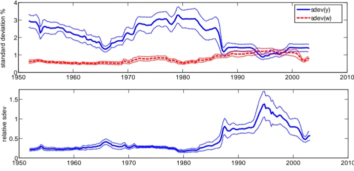
To further illustrate the change in relative volatility of aggregate wages, we plot the volatility of output and aggregate wages over 8-year rolling windows. As the …rst panel of Figure 1 illustrates, the volatility of output fell precipitously in the 1980s whereas the volatility of the aggregate wage steadily increased steadily during the 1980s and 1990s. The standard error bands indicate that both of these changes are signi…cant. As shown in the second panel, the relative volatility of the aggregate wage thus increased dramatically and signi…cantly from the mid-1980s to the mid-1990s. Thereafter, the relative volatility of aggregate wages returns to an intermediate level that remains, however, more than twice as high than the level before the mid-1980s.
We take away two main results from Table 1 and Figure 1. First, as the volatility of output drops during the Great Moderation, the absolute volatility of aggregate wages increases. Second, the drop in output volatility is proportionally much larger than the increase in aggregate wage volatility. The three- to four-fold increase in the relative volatility of aggregate wages is thus driven to a large part by the drop in output volatility. The challenge for any theory is to explain how there can be such a marked fall in output volatility without a similar fall in the volatility of aggregate wages.
2.3
Evidence from other aggregate wage measures
The aggregate wage series from the LPC program is a very broad measure of compensation that includes not only wages and salaries but also stock options. Mehran and Tracy (2001) argue that this may provide a misleading picture of the evolution and volatility of compensation in the 1990s since these stock options are recorded when realized, not when handed out to employees. We
7When computing the volatility of aggregate wages or other macro variables, we drop the …rst and last year to
improve the accuracy of the …lters. Standard errors are computed via the delta method from GMM-based estimates. See the appendix for details.
8The largest p-value of 0.13 occurs for the …rst-di¤erenced wage series. Since …rst-di¤erencing …lters out a
thus check the robustness of our results with three other measures of aggregate hourly measures constructed, respectively, from the CPS May/MORG, the NBER manufacturing database and the Private Economy Labor Quality (PELQ) database.
As described in more detail in the next section, the hourly wage measure from the CPS May/MORG is computed from a representative sample of employed individuals and takes into account wages and salaries, overtime earnings, tips, commissions and bonuses if paid as part of usual compensation. Stock options are not included. The wage measure from the NBER database covers wages of production workers in about 450 four-digit manufacturing industries and is unlikely to be in‡uenced by stock options either. The wage measure from the PELQ database is constructed by Dale Jorgenson and co-authors from a cross-section of CPS and Census data and also excludes stock options (e.g. Jorgenson et al., 2008). The frequency of each of these datasets is annual and spans the period 1973-2006 for the CPS, 1976-2002 for the NBER manufacturing database, and 1976-2000 for the PELQ database.
Table 2 presents the results for the di¤erent aggregate wage series together with an annualized
version of the LPC measure, both in …rst-di¤erenced and HP …ltered form.9 The PELQ measure
shows the largest increases in wage volatility, matching the results of the LPC measure almost exactly. The NBER manufacturing measure and the CPS measure show a somewhat smaller increase in absolute wage volatility, but their relative wage volatility still increases by a factor of 2.5 or more. We can only speculate about the reason for these di¤erences. For the NBER measure, they may be due to the exclusive focus on production workers in manufacturing; for the CPS measure, they may be due to top-coding of large income workers who have seen a more important increase in wage volatility in the post-1984 period than the average worker (see next section). The key point remains, however, that as the volatility of output drops during the Great Moderation, the volatility of all of these wage measures remains stable or even increases slightly. As a result, the relative volatility of aggregate wages increases by a factor of 2.6 to 3.8 between the pre-1984 and the post-1984 period. Another aggregate wage measure to consider is the Average Hourly Earnings (AHE) series from the Current Establishment Survey (CES) of the BLS. As Champagne (2007) and Gali and Van Rens (2009) document, the absolute volatility of the AHE aggregate wage measure declines substantially from the pre-1984 to the post-1984 period and as a result, its relative volatility remains roughly constant. Given the popularity of the AHE measure in both academic research and the business press, it is important to investigate this di¤erence further. We follow Abraham et al. (1998) who document in earlier work that the AHE wage measure diverges greatly from other aggregate wage
9As recommended by Ravn and Uhlig (2002), we set the HP …lter parameter to 6:25. We do not report BP …ltered
results for annual data because the BP …lter requires us to cut ‡uctuations of 2 years or less. This would remove a potentially important part of business cycle ‡uctuations.
measures in terms of its trend over time. For example, whereas the aggregate wage series from the NIPA (basically our QCEW series from the LPC) increases by about 7% over the 1973-1993 period, the AHE measure falls by about 10% over the same period. Abraham et al. (1998) consider three possible explanations for this divergence in trends: (i) problems related the underrepresentation of young establishments in the CES; (ii) di¤erences in the earnings concept used; and (iii) di¤erences in the worker population covered. We examine to what extent any of these three possibilities can
explain the very di¤erent evolution of the volatility of the AHE measure.10
We start with di¤erences in the worker population covered. The AHE measure covers only production and non-supervisory workers, which account for about 80% of total payroll, whereas the aggregate wage measures from the LPC, the CPS May/MORG and the PELQ database are
representative of the entire workforce.11 It is possible that the wage volatility of the 20% of workers
not covered by the AHE increases by so much in the post-1984 period that it more than outweighs the drop in wage volatility in the AHE measure. To assess this possibility, we use the CPS May/MORG data together with occupational de…nitions from the BLS to recreate an hourly wage series for production and non-supervisory workers, as presumably captured by the AHE measure, and an hourly wage series for the remaining private-sector workers. We …nd that the wage volatility of both of these series remains approximatively constant over the pre-1984 and the post-1984 sample period. As a result, the wage volatility of both worker groups relative to the volatility of output increases by a factor of more than 2.5. Abraham et al. (1998) further argue in their paper that employers in the CES often interpret production and non-supervisory workers as employees paid by the hour and other employees that are non-exempt under the Fair Labor Standards Act. Since wages of hourly workers and other non-exempt workers have fallen over their 1973-1993 period, Abraham et al. (1998) conclude that this di¤erence in worker coverage provides the best possible explanation for the divergence in wage trends between the AHE measure and other wage measures. As we show in the next section, however, the relative volatility of hourly workers’ wages also increases substantially in the post-1984 period. It is therefore unlikely that di¤erences in worker population covered can explain the diverging evolution of wage volatility of the AHE measure compared to the di¤erent other aggregate wage measures.
10Another obvious candidate for di¤erences in wage volatility across di¤erent wage series is measurement error.
For measurement error to explain the very di¤erent evolution of wage volatility between the AHE series and the other aggregate wage series, however, it would have to be the case that the measurement error for the AHE series relative to the LPC, CPS May/MORG and PELQ measure decreased substantially. We know of no evidence that points in this direction.
11According to Abraham et al. (1998), the proportion of production and non-supervisory workers in total
Second, we consider di¤erences in earnings concepts. The AHE does not include tips and records commissions and bonuses only if earned and paid in the same period. The CPS May/MORG wage series is the closest to the AHE measure in this respect because it records commissions and bonuses only if they are part of usual earnings. This leaves tips as a di¤erence. As Abraham et al. (1998) report, the BEA estimates tips to be a mere 0.3% of total weekly compensation in 1993. Hence, even if the volatility of tips had increased greatly, this would not explain why the volatility of the CPS May/MORG wage measure increased by such a large amount relative to the AHE wage measure.
Third, we turn to the issue of underrepresentation of young establishments in the CES. As Abra-ham et al. (1998) explain, the CES sample of reporting establishments was not rotated regularly for most of the sample period we consider. Hence, young establishments are typically underrepre-sented. Furthermore, the CES sample grew from about 166,000 establishments in 1980 to about 333,000 establishments in 1993, which is likely to have led to an increase of the proportion of young establishments in the CES sample. While Abraham et al. (1998) conclude that the e¤ect of this expansion on aggregate wage trends is likely to be modest, it is possible that this expansion explains at least part of the di¤erence in the evolution of wage volatility. Absent micro data on the di¤erent CES establishments, however, we cannot investigate this possibility further. The di¤erence in the evolution of wage volatility for the AHE measure relative to the other aggregate wage measures thus remains a puzzle. Given the similarity of results across the LPC, the CPS May/MORG, the NBER manufacturing database and the PELQ database, it appears safe to conclude, however, that the increase in the relative volatility of aggregate wages is a robust feature of the data and not an artifact of some particular measurement of compensation or restriction to a narrow segment of the worker population.
3
A closer look at disaggregated data
To further investigate the increase in volatility of real hourly wages, we take the CPS data and construct wage series for di¤erent groups of workers. We …rst describe important details about the CPS data and then look at the evolution of wage volatility for di¤erent groups of workers. Based on these decompositions, we develop an accounting method that allows us to quantify how much of the increase in the volatility of the aggregate wage is due to increases in wage volatility of di¤erent worker groups.
3.1
CPS data
The CPS is the o¢ cial household-based labor market survey in the U.S. It collects information on roughly 60,000 households about various worker characteristics. Following Lemieux (2006), we use the Dual Jobs Supplement of the CPS May extracts for the 1973-1978 period and the CPS Merged Outgoing Rotation Groups (MORG) for the 1979-2006 period to construct annual series of average
hourly wages and hours of work.12 From the total sample, we drop all unemployed, self-employed,
and individuals under 16 years old. We also remove private household workers, agricultural workers, armed force personnel, and individuals with no data on either earnings or hours. For the remaining sample, we collect a direct measure of the hourly wage rate for all workers paid by the hour (i.e. ’hourly workers’). For workers not paid by the hour (i.e. ’non-hourly workers’), we compute an hourly wage rate by dividing usual weekly earnings by usual weekly hours. We then combine these hourly wage data with the appropriate CPS weights to compute a representative time series for the aggregate non-farm hourly wage rate as well as average hourly wage rates for di¤erent groups of
workers as de…ned below.13
There are two important issues with the CPS data that we need to address for our time-series analysis of wages: topcoding and the 1994 redesign of the CPS. Topcoding in general may lead to biased measures of wage volatility because variations in wages of topcoded individuals cannot be taken into account. Furthermore, there have been several adjustments of the topcoding threshold over time, which may lead to discontinuities in our wage series and overstate the volatility of wage
series.14 To account for topcoding, several researchers have taken a simple adjustment rule and
multiplied topcoded earnings observations by a factor of 1.3 or 1.4. Others have tried to estimate the mean above the topcode based on di¤erent distributional assumptions. The most popular among them is the Pareto distribution approach, which has been shown to provide the best approximation
12The MORG data is available on a quarterly basis. Since the data only starts in 1979, we do not consider the
MORG data in isolation but compute annual averages from the quarterly data and combine them with the May extracts for a longer sample.
13Alternatively, we could have computed hourly wage series from the CPS March Supplements. The CPS March
data would have the advantage that it starts in 1963 rather than 1973. However, before 1976, only weekly earnings can be computed, which is a biased measure of hourly wages if hours worked vary across weeks. Furthermore, as Lemieux (2006) argues, CPS March wage measures are subject to substantial measurement error that are not present in the CPS May/MORG data. The reason for this di¤erence is that the CPS March collects labor earnings only on a yearly basis. The CPS May/MORG, by contrast, asks directly for the wage rate for hourly workers. This seems to yield more precise answers. For these reasons, we refrain from using CPS March data.
14For hourly worker, wages are topcoded at $99.99 per hour, a threshold that is rarely crossed. For non-hourly
workers, weekly earnings are topcoded at $999 before 1989, $1,923 before 1998 and $2,884 thereafter. A substantial share of individuals is above that threshhold at any time of the sample.
of the actual mean in con…dential CPS samples.15 We use a battery of di¤erent topcode adjustment methods and …nd that our volatility results do not di¤er across methods. For simplicity, we thus report all of our results here for topcoded weakly earnings adjusted by a factor of 1.3.
The second important issue is the CPS redesign in 1994, more speci…cally the treatment of weekly overtime earnings, tips, and commissions (OTC). Before 1994, hourly workers were asked to report their hourly wage rate, without a speci…ed question on OTC earnings. After 1994, a
speci…c question was added to hourly workers about weekly OTC earnings.16 The consequence of
this redesign is a potential discontinuity in the wage series for hourly workers, which could lead to an overstatement of the wage volatility in the post-1984 period. To check whether this may be the case, we compute two alternative wage series for hourly workers. First, we simply drop OTC earnings after 1994. Second, we adjust the wage series for non-hourly workers before 1994 with a linear trend so as to correct for any discontinuity. In both cases, all of our results remain robust, meaning that the addition of the OTC question in 1994 for non-hourly workers does not lead to an overstatement of the volatility in CPS wages.
3.2
Wage volatility across di¤erent decompositions
We consider four di¤erent decompositions: (i) skill / gender; (ii) skill / age; (iii) skill / employment
status; and (iv) skill / industry a¢ liation.17 Following Krusell et al. (2000) and many others,
we measure skill by years of schooling. To keep the decomposition manageable, we consider only two groups, de…ning a ’skilled worker’ as someone with a college degree (bachelor) or more, and an ’unskilled worker’ as someone with less than a college degree. The de…nitions of the other decompositions are described below.
For each of the decompositions, we compute an average hourly wage series and follow the same procedure as for the aggregate wage series: …lter the series to extract the business cycle component; split the sample into a pre-1984 and a post-1984 period; compute the volatility of the hourly wage
series both in absolute terms and relative to the volatility of aggregate output.18 Aside from the
15See Feenberg and Poterba (1992), Polivka (2000) and Schmitt (2003).
16For non-hourly workers, the usual weekly earnings include OTC earnings throughout the whole sample. As a
result, the CPS redesign did not a¤ect the usual weekly earnings of non-hourly workers.
17Given the discussion about the e¤ects of deunionization on wage ‡exibility in Section 5, it would be interesting
to do a decomposition along union membership as well. Unfortunately, the CPS MORG does not provide union data before 1983, and for 1981 and 1982 the CPS May contains only very few (respectively no) individuals with information on union membership. This makes it impossible to compute reliable wage series for unionized and non-unionized workers for the pre-1984 sample.
18All results are reported for H-P …ltered data with constant 6:25 as before. We cut o¤ the …rst and last year of
volatility of the hourly wage, we also report the average wage share and the volatility of the hours’ share, de…ned, respectively, as the fraction of total earnings and total hours accounted for by a given worker group (the formal de…nition is provided in Section 3.3). Both of these statistics turn out to be important for the volatility accounting exercise below.
Gender / skill decomposition
Table 3 reports the decomposition for gender and skill. The …rst noticeable change across subsamples is the increase in the relative importance of skilled and female workers (as measured by average wage shares). Second, we observe that the absolute volatility of hourly wages increases for all but skilled female workers for which wage volatility falls slightly. Relative to the volatility of output, however, the volatility of wages increases substantially across all groups. This is especially pronounced for male skilled workers who see their relative wage volatility increase by a factor of 4.5. By contrast to the hourly wage, the volatility of hours’share decreases markedly for all groups. As a result, the relative volatility of hours’share increases by much less and actually falls for both male and female skilled workers.
Age / skill decomposition
Table 4 displays the decomposition for age and skill. Following Gomme et al. (2004), and Jaimovich and Siu (2008), we create three age groups: 16-29 year olds (’young workers’); 30-59 year olds (’grown-ups’); and 60-70 year olds (’old workers’). As the changes in the average wage shares show, there is a substantial shift in the workforce from young to grown-up workers between the pre-1984 and the post-1984 period. In terms of volatility, we …nd that the absolute volatility for all but the young skilled workers decreases. However, this increase is modest for all but the old skilled workers. As a result, the relative volatility of wages still increases strongly for all but this last group. In particular, the relative wage volatility of young skilled workers increases by a factor of 4.5. For hours’share, in turn, the picture is very similar to the gender-skill decomposition: in absolute terms, the hours’share volatility falls substantially for almost all worker groups and thus,
the relative volatility remains on average more or less unchanged.19
Employment situation / skill decomposition
Table 5 shows the decomposition for employment status and skill, where employment status is measured by whether a worker is paid an hourly wage rate or a non-hourly salary in his main job. As for the gender / skill decomposition, the evolution of the average wage share indicates that there is a shift towards a more skilled workforce. The volatility of wages increases for all but the
19As a sidenote, Gomme et al. (2004) and Jaimovich and Siu (2008) document that the volatility of hours displays
a U-shaped pattern with respect to age. As Table 4 shows, the same U-shaped pattern is present for the volatility of hours’share.
non-hourly unskilled group. The relative volatility of wages thus increases markedly for all worker groups. Interestingly, this increase is most pronounced for hourly unskilled workers and non-hourly skilled workers, the two opposites in this decomposition. In terms of hours’share, the situation is similar to the above decompositions: the volatility of hours’share decreases substantially and thus, its change in relative volatility is much more muted than for the hourly wage.
Industry / skill decomposition
Table 6 reports the decomposition for industry a¢ liation and skill. We choose a relatively detailed decomposition into 10 private sector industries and one public administration sector. The importance of the wage share for the service sector increases markedly whereas the wage share of unskilled manufacturing groups decreases. In terms of volatility, we see that the wage volatility of many groups decreases. As for the age / skill decomposition, however, this decrease in volatility is generally modest and thus, the increase in relative volatility of wages remains large for all but communications and public sector workers (both skilled and unskilled). For hours’share, the picture is reversed. Most worker groups see a large decrease in absolute volatility and thus, the relative volatility of hours’share increases only modestly on average.
We take away three stylized facts from the di¤erent decompositions. First, there are important shifts in the workforce as measured by average wage shares. Second, there are substantial di¤erences in the evolution of wage volatility across di¤erent worker groups. The largest increases in volatility occur for male, skilled and young workers. Many other groups, especially in the industry / skill decomposition, see their wage volatility decrease. However, these decreases are relatively modest in absolute terms and thus, the volatility of real hourly wages relative to the volatility of aggregate output increases substantially for almost every worker group. This phenomenon is what we call in the introduction ’The Great Increase in Relative Volatility of Real Wages’. Third and …nally, there is a more substantial decrease in the volatility of hours’share for most worker groups. As a result, changes in the relative volatility of hours’share are on average much more modest. These stylized facts are robust with respect to other decompositions that we attempted with the CPS data (details are available from the authors upon request).
3.3
Volatility accounting
An obvious question coming out of the di¤erent decompositions is how much of the increase in absolute and relative volatility of aggregate wages is due to changes in wage volatilities within the di¤erent worker groups and how much is due to compositional changes of the workforce (i.e. a shift of the workforce towards jobs with more volatile wages). To quantify these e¤ects, we develop an accounting method that allows us to decompose the increase in aggregate wage volatility into
compositional changes, changes in volatilities of hourly wages and hours’ shares, and changes in correlations thereof.
By de…nition, the aggregate real hourly wage wt equals the sum of average real hourly wages
wi;t across worker groups i of some decomposition (e.g. skilled and unskilled), weighted by the
respective hours shares hi;t = Hi;t=Ht; i.e.
wt=
X
i
wi;thi;t,
where Ht and Hi;t denote total aggregate hours worked and hours worked by group i. Next, we let
xi;t = wi;thi;t be the ’wage component’ of worker group i and compute growth rates of the above
decomposition. We obtain log wt wt wt 1 wt 1 =X i xi;t 1 wt 1 xi;t xi;t 1 xi;t 1 X i
si;t 1 log xi;t,
where si;t 1= xi;t 1=wt 1 denotes the ’wage share’of worker group i. Given this decomposition, we
can express the variance of the growth rate of the aggregate real hourly wage as V ( log wt) =
X
i
X
j
COV (si;t 1 log xi;t; sj;t 1 log xj;t):
To make this variance decomposition operational for our accounting exercise, we assume that wage
shares si;t 1 are approximately constant over the sample under consideration; i.e. si;t 1 = si. For
each of the decompositions, we check this approximation and …nd the induced error to be negligible. This allows us to express the di¤erence in aggregate hourly wage variances over two subsamples (denoted 1 and 2) as 2 w;2 2 w;1 = X i X j
si;2sj;2 (xi;2; xj;2) xi;2 xj;2 X
i
X
j
si;1sj;1 (xi;1; xj;1) xi;1 xj;1,
where 2w;2denotes the variance of aggregate wage growth V ( log wt)in subsample 2; (xi;2; xj;2) =
COV ( log xi;t; log xj;t)=
p
V ( log xi;t)V ( log xj;t) denotes the correlation coe¢ cient between
wage component of group i and wage component of group j in subsample 2; and so forth for the
other elements. Our objective is to decompose 2
w;2 2w;1 into (i) changes in wage shares; (ii)
changes in wage volatilities across worker groups; (iii) changes in hours’ share volatilities across worker groups; and (iv) changes in correlation coe¢ cients. As the above expression shows, this is not straightforward because the di¤erent moments enter both additively and multiplicatively. Consider …rst the contribution of changes in wage shares versus the contribution of changes in covariances of the wage components (which captures the remaining three changes). By adding and
substracting di¤erent elements, we can expand the above expression as 2 w;2 2w;1 = X i X j
si;2sj;2 (xi;2; xj;2) xi;2 xj;2 (xi;1; xj;1) xi;1 xj;1
+X
i
X
j
[si;2sj;2 si;1sj;1] (xi;1; xj;1) xi;1 xj;1.
This decomposes the change in the variance of aggregate wages into changes in wage shares given covariances of wage components of the …rst subsample and changes in covariances of wage compo-nents given wage shares of the second subsample. Alternatively, we can expand the above expression as 2 w;2 2 w;1 = X i X j
[si;2sj;2 si;1sj;1] (xi;2; xj;2) xi;2 xj;2
+X
i
X
j
si;1sj;1 (xi;2; xj;2) xi;2 xj;2 (xi;1; xj;1) xi;1 xj;1 .
In this way, we decompose the change in the variance of aggregate wages into changes in covariances of wage components given wage shares of the …rst subsample and changes in wage shares given covariances of wage components of the second subsample. Since there is no particular economic justi…cation to prefer one expansion over the other, we take the average over the two and obtain
2 w;2 2 w;1 = X i X j si;2sj;2+ si;1sj;1
2 (xi;2; xj;2) xi;2 xj;2 (xi;1; xj;1) xi;1 xj;1
+X
i
X
j
(xi;2; xj;2) xi;2 xj;2 + (xi;1; xj;1) xi;1 xj;1
2 [si;2sj;2 si;1sj;1] :
This averaging over two di¤erent extremes is obviously an arbitrary choice. We …nd, however, that all of our robust are robust if we used instead one of the two extremes.
We are left with the decomposition of changes in covariances of wage components into changes of variances and correlation coe¢ cients of average hourly wages and hours’shares. We can express any covariance between wage components of worker group i and j as (xi; xj) xi xj = (wi; wj) wi wj+ (hi; hj) hi hj + 2 (wi; hj) wi hj. Applying the same averaging over the two possible expansions to this expression (see the appendix for details), we obtain the following …nal decomposition of
aggregate wage variances over two subsamples20 2 w;2 2 w;1 = X i X j [si;2sj;2+ si;1sj;1] 2 8 > > > > > > > > > < > > > > > > > > > : " (w i;2;wj;2)+ (wi;1;wj;1) 2 wi;2 wj;2 wi;1 wj;1 + (wi;2;hj;2)+ (wi;1;hj;1) 2 hj;2+ hj;1 2 ( wi;2 wi;1) #(1) + " (h i;2;hj;2)+ (hi;1;hj;1) 2 hi;2 hj;2 hi;1 hj;1 + (wi;2;hj;2)+ (wi;1;hj;1) 2 wi;2+ wi;1 2 ( hj;2 hj;1) #(2) + h
2 wi;2 hj;2+2 wi;1 hj;1 [ (wi;2; hj;2) (wi;1; hj;1)]
i(3) 9 > > > > > > > > > = > > > > > > > > > ; +X i X j
(xi;2; xj;2) xi;2 xj;2 + (xi;1; xj;1) xi;1 xj;1
2 [si;2sj;2 si;1sj;1]
(4)
.
Part (1) is the portion of the change in the variance of aggregate wages accounted for by changes in wage volatility of di¤erent worker groups; part (2) is the portion accounted for by changes in the volatility of hours shares; part (3) is the portion accounted for by changes in correlations coe¢ cients across hourly wages and hours shares; and part (4) is unchanged from before, measuring the portion of the change in the variance of aggregate wages accounted for by compositional changes in the workforce as measured by the di¤erence in wage shares.
The proposed accounting exercise can be implemented for the di¤erence in absolute variances of aggregate wages (described above) as well as for the di¤erence in relative variances of aggregate wages; i.e. 2w;2= 2y;2 2w;1= 2y;1. For the latter, we simply divide each second moment term by 2y;2
or 2y;1, respectively. Note that this leaves the di¤erence in wage shares unchanged, which turns out
to be important for the results.
Tables 7 and 8 show the results of our accounting exercise, both for the change in absolute
volatility of aggregate wages (i.e. 2
w;2 2w;1) and the change in relative volatility of aggregate
wages (i.e. 2
w;2= 2y;2 2w;1= 2y;1). All results are for HP …ltered data. In other words, we substitute
growth rates of hourly wages and hours’shares by their respective HP business cycle component.
This approximation holds extremely well.21
As Table 7 shows, compositional changes account for more than 100% of the increase in the absolute volatility of aggregate wages for all four decompositions discussed in Section 3.2. The contributions of changes in wage volatility, hours share volatility and correlation coe¢ cients, by contrast, di¤er wildly across decompositions. This variation in results should not come as a surprise.
20Note that for i = j, (w
i; wj) wi wj simpli…es to
2
wi, and (hi; hj) hi hj simpli…es to
2
hi Hence, our variance decomposition contains both variances and correlation coe¢ cients. The form of this decomposition is similar to the one proposed in McConnell and Perez-Quiros (2000), Kahn et al. (2002) or Stiroh (2009) for other macro aggregates. However, our decomposition is complicated by the fact that the sum of log hourly wages of di¤erent worker groups does not equal the log of aggregate hourly wages.
For example, the absolute volatility of wages increases substantially for most groups of the gender / skill and the employment status / skill decomposition, but decreases for most groups of the other two decompositions. As a result, the contribution of changes in wage volatility across worker groups to the increase in aggregate wage volatility is strongly positive for the gender / skill and the employment status / skill decompositions, but strongly negative for the other two decompositions. Similar di¤erences explain the large variations in contributions of changes in hours share volatility and correlations across the di¤erent decompositions.
The picture is very di¤erent in Table 8 where we display the same accounting exercise for the change in relative volatility of aggregate wages. Now, for every decomposition, changes in the relative volatility of wages across worker groups account for the bulk of the increase in the relative volatility of aggregate wages. Compositional changes and changes in the relative volatility of hours shares, by contrast, account for no more than 12% (in the employment situation / skill decomposition). This di¤erence in results is due to the fact that the volatility of wages relative to the volatility of output increases strongly for almost all worker groups in each of the decompositions while the change in composition and the change in relative volatility of hours share is generally modest.
3.4
Additional evidence from individual panel data
The decompositions we consider remain averages for workers with broad characteristics (e.g. male and skilled). Hence, it could be that the documented increase in relative wage volatility is the
result of compositional changes within the di¤erent worker groups considered.22 However, starting
with Gottschalk and Mo¢ tt (1994), di¤erent papers using panel data show that income has become considerably more volatile (in absolute terms) on an individual level as well. Dynan et al. (2008) provide an extensive review of this literature and document, using data from the Panel Study of Income Dynamics (PSID), that this increase in individual income volatility (i) occurred within each major age and education group; (ii) stems to a large part from an frequency of large income changes rather than changes throughout the income distribution; and (iii) is predominantly due to increased volatility in labor earnings per hour. Jensen and Shore (2008) extend the analysis of the PSID data and …nd that most of this increase in income volatility can be attributed to individuals with the most volatile incomes, identi…ed ex-ante by high income changes in the past. For the other individuals, income volatility has remained more or less constant.
22Unfortunately, the CPS data does not allow us to discard this possibility because the same individual appears
only for two periods of four months, separated by eight consecutive months during which the individual is left out of the survey.
Our results based on CPS data are consistent with Dynan et al. (2008) and Jensen and Shore (2008) in the sense that we …nd substantial heterogeneity about the change in absolute wage
volatil-ity across the di¤erent decompositions.23 Compositional changes within worker groups may play
some role for this heterogeneity. At the same time, these panel studies report that individual in-come volatility has either increased or remained roughly constant. Since the volatility of output fell by about 60% during the same time period, the volatility of income relative to the volatility of output must have increased substantially. This is entirely consistent with the conclusions from our accounting exercise that the across-the-board increase in relative wage volatility is the main source of the increase in the relative volatility of aggregate wages. The challenge is to come up with a theory that rationalizes both the drop in the volatility of output and the relatively modest changes in the magnitude of wage ‡uctuations across di¤erent workers groups.
4
Wage volatility in general equilibrium
To assess the potential of di¤erent explanations for the change in relative wage volatility, we build a small DSGE model with real wage rigidity. The model is similar to the one presented in Blanchard and Gali (2007) who use it to analyze the implications of wage rigidity for optimal monetary policy. We use the model instead to …rst explore to what extent changes outside of the labor market are capable of generating the observed increase in relative wage volatility. Second, we consider the quantitative e¤ects of changing the degree of wage rigidity on wage dynamics and the economy in general.24
The model is set in a representative agent framework. We thus see our exercise …rst and foremost as an account of aggregate labor market dynamics. However, the e¤ects of changes in wage rigidity that we highlight below apply equally to speci…c labor markets (e.g. the labor market for skilled workers in a given industry). As such, we consider our exploration also as a general …rst pass at explaining why the relative volatility of wages has increased substantially for most worker groups.
23Given that the panel dimension is absent in the CPS data, it is di¢ cult to compare our results further with the
results from PSID studies. Since our data is topcoded (thus missing some of the increase in large income changes noted by Dynan et al., 2008), and self-employed workers (which play an important role in Jensen and Shore’s 2008 analysis) are dropped, our estimates of the evolution of wage volatility are likely to be on the conservative side.
24Gourio (2007), in an unpublished note, proposes a similar model to analyze the e¤ects of changes in the degree
4.1
Model
Since most of the model is standard, we keep the exposition to a minimum and refer the reader to the appendix for a full description. In the following, upper-case variables denote observed macroeco-nomic quantities and lower-case variables denote percent deviations from appropriately transformed steady states.
The economy is populated by 3 types of agents: a continuum of identical worker-households, a
continuum of identical …rms and a monetary authority. Households discount time at rate and
have preferences over consumption and leisure. Period t utility is given by Zt 1 " log Ct Nt1+ 1 + # , (1)
where Ct and Nt are a composite consumption good and hours worked, respectively; Zt 1 is an
exogenous preference shock; and 1= > 0 denotes the Frisch elasticity of labor supply. Households maximize present discounted utility by choosing consumption, hours worked, and investment in
either physical capital Kt+1 (1 )Kt or nominal bonds Bt+1 subject to the budget constraint
Ct+ Kt+1 (1 )Kt+ Bt+1 Rn tPt WtNt+ RtKKt+ Bt Pt + Dt, (2)
where Wt, RKt and Rtn are the real wage rate, the real net rental rate of capital, and the gross
nominal bond return, respectively; Pt is the aggregate price level; and Dt are dividends from a
perfectly diversi…ed portfolio of claims to …rms.
Each …rm produces a di¤erentiated good with constant returns to scale technology
Yt= F (Kt; AtNt), (3)
where At denotes an exogenous labor-augmenting technology shock. The di¤erent …rms’goods are
combined into the …nal composite good according to the Kimball (1995) aggregator.25 Hence, each
…rm is a monopolistic competitor, maximizing pro…ts subject to a downward-sloping demand curve. The monetary authority sets the nominal interest rate according to the following rule
Rtn= (Rnt 1) ( t)(1 ) (Yt=Yt 1)(1 ) y, (4)
where t denotes the gross in‡ation rate of the composite good’s price, and Yt=Yt 1 is the growth
rate of aggregate output.
25Kimball’s (1995) aggregator is a generalization of the Dixit-Stiglitz aggregator and provides ‡exibility in mapping
We impose two market frictions for the determination of equilibrium allocations. First, as is common in the New Keynesian literature, we assume that price setting is staggered following Calvo (1983), with each …rm facing a constant probability in any given period of being able to reoptimize its price. This implies a loglinearized New Keynesian Phillips curve (NKPC) for in‡ation
t= Et t+1+ mct, (5)
with mctdenoting real marginal cost. The slope coe¢ cient in this equation is a nonlinear function
of price setting and demand parameters (see, for example, Eichenbaum and Fischer, 2007).26
Second, we posit as in Blanchard and Gali (2007) that real wages adjust sluggishly according to the following loglinear wage setting curve
wt= wt 1+ (1 )mrst, (6)
where mrst denotes the workers’marginal rate of substitution
mrst= ct+ nt. (7)
Given this wage, …rms hire labor to satisfy their optimality condition
wt= mct+ yt nt. (8)
In words, wages are assumed to be fully allocative but for some unmodelled friction, workers are not on their labor supply schedule as de…ned by the marginal rate of substitution. This formulation of the labor market is admittedly ad-hoc. Yet, there are several reasons for proceeding in this way. First, the simple form of the labor market allows for a straightforward analysis of the e¤ects of increased wage ‡exibility. Second, the next section discusses evidence suggesting that wages indeed play an allocative role over the business cycle. Third, very similar formulations can be derived from more explicit environments; for example (i) an environment with unions that formulate wage demands according to a partial adjustment process (e.g. Blanchard and Gali, 2007); (ii) a model with unobserved ability where …rms pay performance-based wages to a fraction of the workforce (e.g. Lemieux et al., 2008); or (iii) an e¢ ciency wage setup where workers evaluate the fairness of a given wage o¤er by comparing it to their past wage (e.g. Danthine and Kurmann, 2009). Fourth, very similar formulations of wage rigidity are introduced in search-based models of the labor market, motivated by the same type of fairness considerations (e.g. Hall, 2005 and Shimer, 2005). These
26Alternatively, we could have left prices completely ‡exible in which case the model collapses to the RBC
bench-mark. None of the main results below are a¤ected by this simpli…cation. However, it would imply that wages and labor productivity share exactly the same loglinear dynamics, which is not the case in the data.
search-based models have many advantages compared to the present stylized model.27 As we discuss below, however, changes in wage rigidity turn out to be as crucial for search-based models as they are for our more stylized formulation to match observed changes in relative wage volatility.
For capital markets, we keep the competitive markets assumption. The household’s …rst-order condition for investment in physical capital is
ct= Etct+1 rkEtrt+1k zt (9)
and the …rm’s demand for capital is
rkt = mct+ yt kt. (10)
Likewise, the household …rst-order condition for investment in nominal bonds is
ct= Etct+1 (rtn Et t+1) zt, (11)
As is clear from both (9) and (11), the preference shock plays a similar role than a credit shock that drives a wedge between market returns and the intertemporal rate of substitution. Everything
else constant, an increase in zt lowers current consumption, which in turn lowers mrst and wt
(depending on the degree of wage rigidity ).
4.2
Calibration
We calibrate the model to quarterly data. Except for the degree of wage rigidity , the di¤erent
model parameters are kept constant for all simulations and are set as follows. Calibrated model parameters
1= r y
0.333 0.987 0.025 1.000 0.100 0.800 2.000 0.200
The values of ; and are standard (e.g. King and Rebelo, 2000). The unit elasticity of labor
supply is a compromise between the values suggested in the micro and macro literature. The remaining 4 parameters are calibrated in line with estimates from New Keynesian models. The
value of the NKPC slope coe¢ cient lies between the estimates found in limited information
studies such as Gali and Gertler (1999) or Kurmann (2007) and the full-information estimates from
27Aside from providing a clear de…nition of unemployment and labor market ‡ows, search-based models have the
appealing theoretical property that wage rigidities are not necessarily ine¢ cient. In the present formulation, by contrast, we need to appeal to unspeci…ed costs that prevent workers and …rms from renegotiating wages until the marginal rate of substitution equals marginal productivity of labor.
medium-scale macro models such as Smets and Wouters (2007). The monetary policy parameters are close to the ones estimated by Smets and Wouters (2007) for the 1957-2004 period.
For the shock calibration, we also follow the literature and let the technology shock and the preference shock follow independent AR(1) processes
at = aat 1+ "at with "at iid (0; 2"a)
zt = z zt 1+ " zt with " zt iid (0; 2" z)
We estimate the two parameters for each process directly from the data. For the technology shock process, we use a quarterly approximation of the total factor productivity measure constructed by Basu, Fernald and Kimball (2006), which controls for variable factor utilization. We convert this
measure into logarithms, subtract a linear trend and then estimate a and "a by ordinary least
squares (OLS).28 For the preference shock process, we measure zt as the residual from the Euler
equation for nominal bonds in (11); i.e. zt = Et ct+1 (rnt Et t+1).29 The nominal short-rate
in this equation is measured by the 3-month treasury bill rate. Expectations of future consumption growth and in‡ation are estimated from a bivariate VAR in the two variables, with consumption being measured by real chain-weighted per capita expenditures of non-durables and services and
in‡ation being measured by the growth rate of the GDP de‡ator.30 As for total factor productivity,
we subtract a linear trend from the obtained series of zt and then estimate z and " z by OLS.
We limit the …rst observation for all data series to 1953:2 because Treasury bill rates were not market-determined until the 1951 Treasury-Fed Accord, and because we want to avoid the extreme swings in in‡ation during the Korean War period. The point estimates for the pre-1984 and the
28Substracting a linear trend implies that total factor productivity has a deterministic exponential growth rate, as
assumed for example in King and Rebelo (2000). Our results are robust when we apply a higher-order detrending procedure.
29Alternatively, we could measure z
t as the residual from the investment Euler equation in (9). There are two
reasons we prefer the bond Euler equation. First, the rental rate of capital in the investment Euler equation has to be inferred from macroeconomic quantities using the …rm’s capital demand condition in (10). Both the real marginal cost and capital stocks are di¢ cult to measure and thus, we have less con…dence in the resulting series for the rental rate of capital than bond prices and in‡ation, which are directly observable in the data. Second, the investment Euler equation may be a¤ected by investment-speci…c technology shocks. Primiceri et al. (2006) argue that such investment-speci…c shocks neutralize a large part of preference shocks, which would lead to a substantially smoother series for zt. These investment-speci…c shocks do not enter into the bond Euler equation.
30Based on Schwarz’ Bayesian Information Criterion (BIC), we select a VAR in 5 lags. The di¤erent results are
post-1984 period are31
Estimated driving processes
a "a z " z
pre-1984 0.9788 0.0094 0.7956 0.0033
post-1984 0.9738 0.0057 0.8951 0.0020
Both shock processes become less volatile in the post-1984 period by about 40%. This drop in volatility of exogenous driving forces is robust across many di¤erent model and shock speci…cations (e.g. Smets and Wouters, 2007) and provides the basis of the ’good luck hypothesis’of the Great Moderation, a point to which we return below. For the baseline calibration, we set the di¤erent shock parameters to their pre-1984 estimates and then vary them later to their post-1984 estimates. The …nal parameter we need to calibrate is the degree of wage rigidity . Since the wage setting
equation in (6) is reduced-form, we cannot calibrate it based on micro evidence. We thus set such
that the model calibrated with the above parameter values and shock estimates for the pre-1984
period matches the standard deviation of HP …ltered output. This yields a value of = 0:85,
implying that the pre-1984 period was characterized by a substantial degree of wage rigidity.
4.3
Simulations
We compute several simulations of the model to illustrate the importance of increased ‡exibility in wage setting. First, we discuss how model under the baseline calibration matches salient labor market dynamics in the pre-1984 period. Second, we assess to what extent a reduction in the volatility of exogenous shocks can generate an increase in the relative volatility of wages. Third,
we consider the e¤ects of lowering the degree of wage rigidity by setting = 0:15 while keeping
the shock processes at their pre-1984 calibration. This decrease in wage rigidity is motivated in part by direct evidence from Kahn (1997) who uses PSID data to show that the frequency of wage adjustments has increased over the past decades. Furthermore, we discuss in the next section di¤erent sources that may have led to this type of increase in wage ‡exibility. At the same time, neither Kahn’s (1997) study nor the evidence discussed in the next section allows us to conclude
that wage setting has become almost completely ‡exible as implied by = 0:15. Rather, we want
to assess with this simulation the extent to which increased wage ‡exibility is capable of a¤ecting
labor market dynamics.32 Fourth, we keep = 0:15and adapt the shock calibration to the post-84
31For both sub-periods, the correlation between the innovations is negligible (0.11 and -0.03, respectively). Hence,
our assumption that the two shock processes are independent is valid.
estimates so as to assess how changes in the relative importance of shocks interact with increased wage ‡exibility.
While the main focus of our investigation is to quantify the potential of increased wage ‡exibility to generate the observed increase in relative volatility of wages, we are also interested in assessing whether our theory can replicate other prominent changes in labor market dynamics. As noted in the introduction, the Great Moderation period is also characterized by an increase in the relatively
volatility of hours worked and a fall in the correlation of labor productivity with output and hours.33
The …rst three columns of Table 9 document these changes. The volatility of both hours and labor productivity has increased relative to output. However, this increase in relative volatility is far smaller than the relative increase in volatility of aggregate wages. The correlation of labor productivity with output has turned from robustly positive to zero whereas the correlation with hours has turned substantially negative. A similar development applies to wages, which have become mildly negatively correlated.
Baseline calibration
Simulation 1 in Table 9 displays the second moments generated by the model for our baseline
calibration with = 0:85 and the shock processes set to their pre-1984 estimates. As discussed
above, the degree of wage rigidity is chosen such that the model matches the pre-1984 volatility of output in the data. Despite its simplicity, the model does a surprisingly good job in matching other pre-1984 data moments. In particular, the model generates a relative volatility and correlation coe¢ cient of wages that is only slightly above the values in the data. The relative volatility of labor productivity and its correlation with output and hours are also close to their data counterparts.
Smaller shocks
We now change the calibration of the two shock processes to their post-1984 estimates while keeping all of the other parameters at their baseline values. This is the ‘good luck hypothesis’of the Great Moderation, proposed by Stock and Watson (2003) or Sims and Zha (2006) among many others, which says that most of the decrease in business cycle volatility in the post-1984 period can be attributed to smaller shocks. As Simulation 2 in Table 9 shows, the smaller estimates of the two shock processes leads to a substantial fall in output volatility of about 40% as well as a fall in the cyclicality of wages and labor productivity. Hence, the ‘good luck hypothesis’is quite powerful in accounting for the Great Moderation and is consistent with some of the changes in labor market dynamics highlighted by Stiroh (2009), Barnichon (2008) and Gali and Gambetti (2009). At the same time, the decrease in shock volatility in the post-1984 period leads to a substantial fall in the volatility of wages such that the relative volatility of aggregate wages hardly changes. The ’good
luck hypothesis’on its own thus fails to account for the sizable increase in the relative volatility of wages that we observe in the data.
To understand these results, it is useful to consider a graphical illustration of the labor market. Figure 2a depicts the response of wage setting (6) and labor demand (8) to a positive technology
shock in the w n space. Starting from point A, the technology shock moves labor demand to the
right and shifts up the wage setting curve due to the positive income e¤ect. Because of consumption
smoothing, this income e¤ect is relatively modest. A high degree of wage rigidity (i.e. = 0:85)
thus implies that wages adapt slowly and …rms increase labor input (and production) by a lot, as depicted by the move to equilibrium point B. Smaller technology shocks change the absolute but not relative size of the shifts in the two curves. The magnitude of adjustments in w compared
to n (and output) thus remain more or less unchanged.34 Figure 3a illustrates the e¤ect of a
preference shock on labor demand and wage setting. Everything else constant, the preference shock reduces current consumption, which implies a negative income e¤ect that shifts down the wage setting curve. Aside from negligible e¤ects from dynamic capital adjustments (not shown here), the labor demand schedule remains una¤ected and thus, the economy adjusts from point A to its new equilibrium at point B. Similar to the technology shock, smaller preference shocks result in smaller shifts of the wage setting curve. But as long as the degree of wage rigidity and the wage elasticity of labor demand remain unchanged, the relative magnitude of adjustments in w and n remain more or less the same. This explains why changes in technology and preference shocks have hardly any e¤ect on the relative volatility of wages. By contrast, changes in technology and preference shocks may have important e¤ects on the cyclicality of wages and labor productivity. As the two …gures reveal, technology shocks imply that both wages and labor productivity co-move with hours, whereas preference shocks imply exactly the opposite. When preference shocks become relatively more important, the correlation of wages and labor productivity with hours (and thus output) falls and may even become negative. As Simulation 2 in Table 9 shows, this is exactly what happens in our model for the post-1984 estimates of the two shocks.
The graphical illustration suggests that similar conclusions apply for other exogenous shocks that shift either the wage setting curve or the labor demand but do not a¤ect their respective wage elasticities. Likewise, structural changes outside of the labor market (e.g. changes in monetary policy) should have only a negligible impact on the relative volatility of wages. We assess this conjecture with the larger DSGE model of Smets and Wouters (2007) that contains several real and
nominal frictions and seven di¤erent exogenous shocks.35 We …rst simulate the model using the
34Our explanation ignores dynamic e¤ects coming through movements in capital stocks. Since capital stocks move
slowly over the business cycle and account for a relatively small part of production, these e¤ects are negligible.
estimates for the 1966-1979 period reported by Smets and Wouters and then change the calibration of the seven exogenous shock processes to their 1984-2004 estimates (keeping all other parameters constant). The HP-…ltered volatility of output drops from 1.82 to 1.26, thus con…rming the ’good luck hypothesis’of the Great Moderation. At the same time, the volatility of real wages falls from 0.84 to 0.79, implying an increase in relative wage volatility from 0:45 to 0:62. While this increase is somewhat larger than for the more stylized DSGE model above, it remains far from the increase in relative wage volatility observed in the data. Furthermore, when we change the calibration of the monetary policy rule in the Smets-Wouters model from the 1966-1979 estimates to the 1984-2004
estimates, we …nd that the impact on the relative volatility of wages is very small.36 We therefore
conclude that the observed increase in relative wage volatility is unlikely to come from changes outside the labor market (e.g. smaller exogenous shocks or di¤erent monetary policy).
Increased wage ‡exibility
To assess the e¤ects of increased wage ‡exibility in isolation, we reset the calibration of the shock processes in our small DSGE model to their pre-1984 estimates and reduce instead the degree
of wage rigidity from = 0:85 to = 0:15. As Simulation 3 in Table 9 shows, this simple increase
in wage ‡exibility is capable of generating a substantial increase in the relative volatility of wages. More speci…cally, the increase in relative wage volatility is due to a modest increase in the absolute volatility of wages (not shown) and a drop in output volatility of about 35%. Hence, the increase in wage ‡exibility not only leads to an increase in wage volatility but also implies smaller business cycle ‡uctuations. At the same time, the increase in wage ‡exibility leads to a counterfactual increase in the correlations of wages and labor productivity with output and hours.
As before, it is useful to consider a graphical illustration to understand the mechanisms behind these results. Figure 2b depicts the impact of a positive technology shock in a labor market with
high and low degrees of wage ‡exibility. The low wage ‡exbility case (i.e. = 0:85) is exactly the
same case than in Figure 2a; i.e. a positive technology shock shifts out the labor demand curve and the economy moves along a relatively ‡at wage setting curve from point A to point B. Under ‡exible lagged in‡ation, external habit persistence in consumption, investment adjustment costs, variable capital utilization and …xed costs in production. The exogenous shocks are a TFP shock, an investment-speci…c technology shock, a government spending shock, a labor supply shock, an intertemporal preference shock, a price markup shock, and a monetary policy shock. We simulate a loglinearized version of the model using the DYNARE code that Smets and Wouters supply on the AER website.
36Clarida et al. (2000) and Boivin and Giannoni (2006) among others argue that starting in the 1980s, U.S.
monetary policy has become substantially more aggressive with respect to in‡ation. However, estimates by Smets and Wouters (2007) contradict this result. In our small DSGE model as well as in the Smets-Wouters model, we …nd that changes in the monetary policy response to in‡ation have have only a small impact on output volatility and do not matter for the relative volatility of wages.