HAL Id: hal-00737390
https://hal.archives-ouvertes.fr/hal-00737390
Submitted on 1 Oct 2012
HAL is a multi-disciplinary open access
archive for the deposit and dissemination of
sci-entific research documents, whether they are
pub-lished or not. The documents may come from
teaching and research institutions in France or
abroad, or from public or private research centers.
L’archive ouverte pluridisciplinaire HAL, est
destinée au dépôt et à la diffusion de documents
scientifiques de niveau recherche, publiés ou non,
émanant des établissements d’enseignement et de
recherche français ou étrangers, des laboratoires
publics ou privés.
SyDiG: uncovering Synteny in Distant Genomes
Géraldine Jean, Macha Nikolski
To cite this version:
Géraldine Jean, Macha Nikolski. SyDiG: uncovering Synteny in Distant Genomes. Int. J. of
Bioin-formatics Research and Applications, 2011, pp.43-62. �10.1504/IJBRA.2011.039169�. �hal-00737390�
SyDiG: Uncovering Synteny in Distant Genomes
G´
eraldine Jean* and Macha Nikolski**
Friedrich Miescher Laboratory of the Max Planck Society, Tbingen, Germany
E-mail: [email protected]
∗Corresponding author
CNRS/LaBRI, Universit´e Bordeaux 1, 351 cours de la Lib´eration,
33405 Talence Cedex, France E-mail: [email protected]
Abstract:
Current methods for detecting synteny work well for sets of genomes with high degrees of inter- and intra-species chromosomal homology, such as mammals. In this paper we define a new algorithm for synteny computation. The main originality of this method is that it is well-suited to genomes covering a large evolutionary span. It is based on a three-step process: identification of initial microsyntenic homologous regions, extension of homologous boundaries using a transitivity relation, and reconstruction of syntenic blocks by identification of groups of homologous genomic segments that are conserved in every subject genome. Our method performs as well as GRIMM-Synteny on mammalian genomes, and outperforms it for clades with much greater evolutionary distances such as the Hemiascomycetous yeasts. The analysis of the algorithms and computed results pinpoints the fact that direct DNA alignments and anchor computation do not provide a sufficient support for synteny recovery in clades covering large evolutionary distances.
Keywords: synteny; algorithm; multiplicon.
Biographical notes: G´eraldine Jean received her PhD in Computer Science, specialty Bioinformatics at the University of Bordeaux. She currently holds a postdoctoral position at Friedrich Miescher Laboratory of the Max Planck Society, Tbingen. Her research interests include issues related to genome evolution and in particular various rearrangement models as well as algorithms in machine learning. She has published research paper at national and international levels, as well as conference proceedings.
Macha Nikolski has received her doctoral degree in Computer Science from the University of Bordeaux on the subject of binary decision diagrams and their application to the reliability analysis and has subsequently worked for Synopsys, before returning to public research to a position of a Research Scientist with the Centre National de Recherche Scientifique (CNRS). In particular she has worked in two distinct but related subjects: algorithms for pattern recognition, inference, and search for optimal solutions in large search spaces; and modeling, for building rigorous descriptions of complex dynamic Copyright c 2009 Inderscience Enterprises Ltd.
systems and establishing formal properties about their behaviors. She has published research paper at national and international levels, conference proceedings as well as chapters of books.
1 Introduction
Comparative analysis of complete genomes has over the past ten years provided increased understanding of the processes and mechanisms of evolution, development, and gene regulation. One area where significant insight has been obtained is genome rearrangements, where the mechanisms of chromosomal dynamics have been explored through comparison of chromosomal maps within and between species. A key prerequisite for such studies is the accurate identification of genome synteny, since conserved gene order between related species indicates chromosomal homology inherited from their common ancestor. Once carefully identified, synteny information is used for computing rearrangement distances (Hannenhalli and Pevzner, 1995) or scenarios (Tesler, 2002), inferring the least common ancestor and rearrangement trees (Bourque and Pevzner, 2002). The implications of the analysis of genomic synteny can reach even further, providing insights into the manner by which evolution proceeds. This latter topic has generated a quite lively debate on the differences between random breakage and fragile breakage models of evolution (Pevzner and Tesler, 2003a,b; Trinh et al., 2004).
Nadeau and Taylor (Nadeau and Taylor, 1984) were the first to define conserved segments as segments having a preserved gene order with no rearrangements between them. Synteny blocks are built of these conserved segments, smoothing over the noise due to microrearrangements. These blocks constitute gene markers that are the starting points for further analysis.
The focus of this paper is the computational identification of genome synteny in complete sequences of distant genomes. A number of methods has been developed in this area. They can be classified in two main categories: alignment-based and profile-based methods.
The most commonly used methods are alignment-based, such as CHAINNET (Kent et al., 2004) and GRIMM-Synteny (Pevzner and Tesler, 2003a; Bourque et al., 2004, 2005). They determine synteny blocks from an initial signal provided by BLASTZ alignments of nucleotide sequences (Schwartz et al., 2004). Since many pairwise relations between DNA segments identified in this manner will be spurious, for example due to domain conservation in protein coding genes, alignment-based methods apply strict filtering policies to link related alignments and remove the spurious ones. Such techniques have been applied with success to sets of mammalian genomes and fly genomes, sets which have a high degree of chromosomal homology,1 and significant conservation in DNA sequences. Such
cases of closely related genomes are of course extremely interesting, particularly in biomedical applications, but they are the ‘low-hanging fruit’ for synteny detection. The profile-based i-ADHoRe routine (Simillion et al., 2004, 2008), extends the pairwise ADHoRe method of (Vandepoele et al., 2002) by iteratively building profiles of intervals of syntenic genes, that are used to search the same genome(s)
again to determine “higher level” multiplicons. This method was originally developed to identify multiple rounds of whole genome duplication in Arabidopsis thaliana, events that leave overlapping signals of self-similarity as is also seen in the genomes of Tetraodon nigroviridis (Jaillon et al., 2004) and Paramecium tetraurelia (Aury et al., 2006). In this method the initial signal is provided by Blastp alignments of predicted translation products, and genomes are represented as lists of genes. The algorithm essentially looks for statistically significant pairs of intervals in these lists with similar gene order and contents. These segments of chromosomal homology are called multiplicons. Multiplicons of level n are used to define profiles, lists of genes defining a consensus between the two intervals in the multiplicon, that are used again in pairwise comparisons with each of the target genomes. The result are multiplicons of level n + 1, and so on.
Both of these existing methods work well on the cases that they were designed for, but perform poorly on the increasingly more common case of sets of related species with highly divergent or extensively reshuffled genomes (see section 3 for comparisons). Recent improvements to sequencing technology are making it feasible to obtain complete sequences from a large number of species of biotechnological interest, and global detection of synteny in such groups is of great practical use for studying chromosome dynamics linked to, e.g. quantitative traits. Despite their phylogenetic relations, such groups of species may by highly divergent. The industrially useful Hemiascomycete yeasts, for example, despite their small, compact genomes and similar ecological niches, are evolutionarily distant. With GC contents ranging from 40% to 52% and an average amino-acid identity of 20% (Dujon, 2006), alignment of DNA sequences is not informative. While alignment of translation products does provide a recognizable signal for gene homology, extensive map reshuffling leads to quite small syntenic segments of 10-15 genes, and iterated profile searching finds few segments conserved in many species (see section 3).
In this paper we present a new method called SyDiG (Synteny in Distant Genomes) that has the ability to handle species having a large evolutionary span. It requires complete genome sequences and infers inter-species synteny in the general case of N ≥ 2 genomes. It follows a three-step process. First, we perform a pre-processing step that consists in determining orthologous genes and, from those, in computing multiplicons of level two. Second, using a novel graph encoding of homology between genomic segments and overlaps of multiple segments on the same chromosome, we extend certain homology relationships at the boundaries of segments by transitivity. Finally, we use the initial orthology information and the identified supplementary homologous elements in order to reconstruct synteny blocks. In the rest of the paper, when speaking of homologous groups we understands the subdivision of these groups in subgroups of orthologs by the SONS method.
In what follows, we present in the first section a formal definition of the SyDiG method and its algorithms. In the second section, we compare Grimm-Synteny and SyDiG on both mammal and yeast genome sets. Finally, in the third section, we present a practical application to Hemiascomycetous yeasts that leads to the rearrangement analysis presented in (Jean et al., 2009).
2 SyDiG algorithm
2.1 Pre-processing
The starting point for synteny identification is the definition of pairwise orthology relationships between genomes. We use our consensus clustering algorithm from (Nikolski and Sherman, 2007) on a mix of complementary partitions (see section 3.3), although raw clustering methods can be used such as (Enright et al., 2002). Furthermore, within these homolgous groups, orthologous subgroups are indentified by the SONS method (Dujon et al., 2009). While in principle sequence similarity can generally detected either at the DNA level or by aligning the translation products of coding sequences, in practice for distant genomes only the latter recovers significant similarity. In this case, one essentially constructs comparative genome maps and the study of gene order makes it possible to detect homology even for highly divergent chromosomic regions. This is exactly the role of the ADHoRe method briefly described above (Vandepoele et al., 2002; Simillion et al., 2004, 2008).
Recall that a multiplicon is formed by one or several homologous genomic segments and its level indicates the number of iterations used to obtain it. In SyDiG we use i-ADHoRe to identify short (microsyntenic) segments as a starting point, but restricted to pairwise computations and thus to computing only level two multiplicons. We will call these segments simply ‘multiplicons’ in the rest of the paper even though more than one genome is involved. The restriction to level 2 multiplicons comes from an empirical observation that use of profiles provides little benefit and, by stringently requiring a synteny relation to have exactly the same boundaries in many species, it retains few segments at every iteration.
Notice that i-ADHoRe determines the multiplicons based on gene order. Hence, the coordinate system used is at gene level: each element of a genomic segment is mapped to a gene and each chromosomic segment is delimited by two genes, one on each side. Multiplicons obtained by i-ADHoRe correspond to homologies between two genomic segments (belonging to the same genome or not). The goal now is to refine these homologies into synteny blocks for the set of considered genomes {G1, .., GN}. We do this by analyzing the composition of each multiplicon
and computing the synteny blocks using transitivity relations.
2.2 Synteny graph
The first step is to assemble all the information contained in the multiplicons into a graph. This graph has to represent two types of information: first, homology between genomic segments; second, possible overlaps between multiple segments of the same chromosome. Let {G1, .., GN} be the set of genomes for which we want
to compute synteny blocks and M be the set of multiplicons obtained by ADHoRe for these genomes.
For the needs of the method, we propose a more formal definition of the notion of multiplicon. Let M = hI1, I2, Ai be a (level two) multiplicon where I1 and I2
denote the genomic segments that it contains, and A is the set of anchors within it. We note a genomic segment Ii as a sequence of genes Ii= (gib, .., gei) such that
gi
segment Ii is a pair hpj, cji such that pj is its relative position on the chromosome
cj. If two genes g1i ∈ I1 and gj2∈ I2 form an anchor in M , then hgi1, g 2 ji ∈ A.
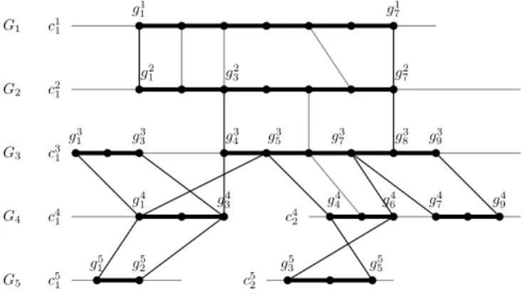
Figure 1 shows an example of multiplicons for N = 5 genomes. This same example will be followed through the paper.
G1 c1 1 g1 1 g71 G2 g2 1 g32 g72 c2 1 G3 g3 1 g 3 3 g 3 4 g 3 5 g 3 7 g 3 8 g 3 9 c3 1 G4 g4 1 g34 g44 g64 g74 g49 c4 1 c42 G5 g5 1 g52 g53 g55 c5 1 c52 b b b b b b b b b b b b b b b b b b b b b b b b b b b b b b b b b b b b b
Figure 1 Level 2 multiplicons for genomes {G1, .., G5}. Each genome Gi is shown on
a separate line with chromosomes denoted by ci
1, ci2,.., cik (k the total number
of chromosomes for Gi). A genomic segment (gij, gj+1i , ..., gk−1i , g i
k) on Gi is
represented by a bold line on the chromosome and is explicitly delimited by its boundaries gi
j and gik. Dots along chromosomes represent gene locations. A
grey (dark, respectively) line materializes an anchor formed by genes (gene boundaries, respectively) at its extremities.
The synteny graph G is defined from the set M of multiplicons for the N genomes under study.
Definition 2.1: A synteny graph G = (V, E) is a non-oriented edge-colored graph such that
- V = {gi
j | gji ∈ Ii∈ M ∈ M} is the set of all genes participating in a
multiplicon,
- E is the edge set such that ∀e = {gi
n, gjm} ∈ E either gin and gjm form an
anchor in a multiplicon of M (dashed edge), or gi
n and gjmare consecutive on
the same chromosome (black edge).
In this graph, we can distinguish three types of vertices: (1) boundary vertices correspond to gene boundaries of genomic segments participating in a multiplicon, (2) anchor vertices correspond to genes that form an anchor with some other gene and are not boundaries of any genomic segments, (3) interleaving vertices are the other vertices that are neither a boundary nor an element of an anchor.
Note that boundary vertices always form an anchor, since ADHoRe computes multiplicons in such a way that extremities of genomic segments that define them are determined by the leftmost and rightmost coordinates of their anchors. Thus, a gene can be both a boundary of one or several genomic segments taking part in
multiplicons and a simple anchors in other segments. An anchor vertex is a gene that forms an anchor strictly inside one or several multiplicons.
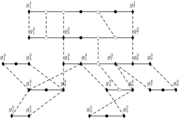
Figure 2 shows the synteny graph obtained for the 5 genomes and their multiplicons of figure 1. g1 1 g71 g2 1 g32 g72 g3 1 g 3 3 g 3 4 g 3 5 g 3 7 g 3 8 g 3 9 g4 1 g34 g44 g64 g74 g49 g5 1 g 5 2 g 5 3 g 5 5 l l l l l l l l l l l l l l l l l l l l l l b c bc b c bc b c b c b c b c b b b b b b b
Figure 2 Synteny graph obtained for the data shown on figure 1. Dashed edges represent homologies while black ones represent gene adjacency. Boundary vertices (anchor vertices, and gene vertices, respectively) are represented by diamonds (white circles and full circles, respectively).
2.3 Extension of homologous boundaries
The synteny graph represents gene relationships within and between genomes: physical relationships are modeled by black edges, which represent gene adjacencies, while dashed edges model homology information contained in multiplicons. From synteny graph, we define two kinds of dependency between elements.
2.3.1 Extended segments
Genomic segments taking part in multiplicons can be physically dependent, since some of them overlap. It is from this kind of dependency that we can infer new homology relationships by combining the information contained in multiplicons related by overlapping genomic segments. Thus, we isolate the set of genes that are dependent only due to chromosomic overlaps. All of these genes will belong to the same extended segment.
Definition 2.2: An extended segment for a given genome is a maximal genomic segment Imax= (gb, .., ge) defined from the set of genomic segments {I1, .., Ik}
belonging to the same chromosome c such that
(i) gb= hpbmin, ci ∈ Ii with 1 ≤ i ≤ k such that pbmin = min({pi | gi= hpi, ci ∈
Ii,1 ≤ i ≤ k}),
(ii) ge= hpemax, ci ∈ Ii with 1 ≤ i ≤ k such that pemax = max({pi | gi= hpi, ci ∈
(iii) 2 consecutive genes on the extended segment belong to the same genomic segment: ∀gi, gi+1∈ Imax, ∃I ∈ {I1, .., Ik} such that gi∈ I and gi+1∈ I,
(iv) the extended segment satisfies the criterion of maximality: ∀I 6∈ {I1, .., Ik} and
∀j ∈ [1, k], I and Ij do not overlap.
The set of extended segments obtained for a given synteny graph G is computed from the connected components of the subgraph of G induced by the black edges of G. In fact, the resulting subgraph can be decomposed into paths that correspond to extended segments.
The synteny graph of figure 2 contains 9 extended segments, namely: - S1 1 = (g 1 1, .., g 1 7) belonging to G1, - S2 1 = (g 2 1, .., g 2 7) belonging to G2, - S3 1 = (g 3 1, .., g 3 3) and S 3 2 = (g 3 4, .., g 3 9) belonging to G3, - S4 1 = (g 4 1, .., g 4 3), S 4 2 = (g 4 4, .., g 4 6) and S 4 3 = (g 4 7, .., g 4 9) belonging to G4, - S5 1 = (g 5 1, .., g 5 2) and S 5 2 = (g 5 3, .., g 5 5) belonging to G5.
2.3.2 Groups of homologous genes and boundaries
The goal of our algorithm is to determine synteny blocks for N genomes under study. We use transitivity of the relation defined by the multiplicons in order to solve the missing homologies between genomic segments. Thus, if I1 is homologous
to I2 that is itself homologous to I3, we consider that I1 and I3 are also
homologous. Not all homologies are that simple to solve. For example, in figure 1, the genomic segment I2
2 = (g 2 3, .., g
2
7) of genome G2 does not have a homolog
(direct or by transitivity) with any genomic segment of genome G1. However, I22
is included in I1 2 = (g
2 1, .., g
2
7) that itself is homologous with I 1 1 = (g 1 1, .., g 1 7) of G1.
This homology makes it possible to deduce a new boundary in G1 that “cuts” I11
into two distinct intervals such that one of them is homologous with I2 2.
Recovering homology relationships between genomic segments can then be reduced to looking for specific genes that are boundaries, and reconstructing the corresponding genomic segments. In order to do that we first partition genes forming at least an anchor in groups of homologous genes and in parallel, by considering only the set of gene boundaries, groups of homologous boundaries. Definition 2.3: Groups of homologous genes are a partition of genes forming at least one anchor such that a part of this partition is a set of genes that are either directly homologous, or that share a gene with which they form an anchor.
Definition 2.4:
Groups of homologous boundaries are a partition of gene boundaries such that a part of this partition is a set of boundaries that are either directly homologous, or that share a gene with which they form an anchor.
homologous boundaries homologous genes g1 1, g 2 1 g 1 1, g 2 1 g1 7, g 2 7, g 3 8 g 1 2, g 2 2 g3 1, g 4 1, g 5 1, g 3 5, g 4 4, g 5 5 g 1 5, g 2 6 g3 3, g 4 3, g 5 2, g 3 4, g 2 3 g 1 7, g 2 7, g 3 8 g5 3, g 4 6, g 3 7, g 4 7 g 2 5, g 3 6, g 4 5 g3 9, g 4 9 g 3 1, g 4 1, g 5 1, g 3 5, g 4 4, g 5 5 g3 3, g 4 3, g 5 2, g 3 4, g 2 3, g 1 3 g5 3, g 4 6, g 3 7, g 4 7 g3 9, g 4 9
Table 1 Groups of homologous boundaries and genes obtained from the synteny graph of figure 2
Groups of homologous genes obtained for a given synteny graph G are computed from the connected components of the subgraph of G induced by the anchor and boundary vertices, and the dashed edges of G rather than groups of homologous boundaries of G are computed from the connected components of the subgraph of G restricted to boundary vertices and the dashed edges of G. The group of homologous boundaries is obtained for a given synteny graph G, in an analogous way, from the the subgraph of G induced by the boundary vertices, and the dashed edges of G.
Starting from the synteny graph from figure 2, we obtain groups of homologous genes and groups of homologous boundaries shown respectively in table 1.
2.3.3 Adding and positioning of new boundaries
The next step is to check each boundary to see whether it creates new boundaries in other genomes. Each extended segment is a genomic segment defined by a maximal set of overlapping genomic segments. Hence, in each extended segment there exist boundaries of genomic segments that are included in others. For example, boundary g2
3 of I 2
2 is included in the interval I 1
2 of the extended segment
S2
1. However, genomic segment I 1
1 homologous to I 1
2 does not contain any boundary
homologous to g2
3. This is precisely the situation where the need for adding new
boundaries arises. In order to do this we search in the groups of homologous genes for a boundary homologous to g2
3 in I 1
1 (see table 1). In this case, we find the gene
g1 3.
The algorithm add boundaries implements this operation. Function extended segment returns the extended segment to which a given genomic segment belongs. In the case of the addition of a supplementary boundary, if the current boundary has no homologous gene in the target genomic segment, then it is necessary to pick a gene in this segment as the homologous one. This is done by the routine locate: the homologous gene is the one that is proportionately located
in the target segment at the same place than the current boundary in its genomic segment.
Algorithm 1add boundaries(S) Require: Set of extended segments S
Ensure: Set of extended segments S with new boundaries 1: Let B be the set of boundaries for S
2: whileB 6= ∅ do 3: b= shif t(B)
4: Let I be the set of genomic segments in which b is included 5: for allI∈ I do
6: for allI′ such that ∃M = hI, I′, Ai ∈ M do
7: if 6 ∃ bh∈ I′ such that bh and b are two homologous boundaries then 8: if ∃ ba∈ I′ such that ba and b are two homologous genes then 9: S′= extended segment(I′,S)
10: Mark ba as boundary in S′
11: Add ba in B
12: Add ba in the group of boundaries homologous to b
13: else
14: S′= extended segment(I′,S) 15: locate(bnew, S′)
16: Mark bnewas boundary in S′
17: Add bnew in B
18: Add bnew in the group of gene homologous to b 19: Add bnew in the group of boundaries homologous to b
20: end if 21: end if 22: end for 23: end for 24: end while 25: return S
For the example of figure 1, six new boundaries are added. All the new boundaries are shown in figure 3. The resulting groups of homologous boundaries are shown in table 2.
2.4 Reconstructing synteny blocks
Once boundary homology is completely solved, we define the genomic segments and their homology relations. In an extended segment, two boundaries form a genomic segment that is necessarily homologous with at least one other genomic segment. In order to obtain genomic segments that are disjoint for a given chromosome, it is sufficient to go through each extended segment in order, where two successive boundaries delimit a genomic segment. Then, from boundary homology, we deduce homologies between segments delimited by these boundaries. This implies finding the two corresponding boundaries in another genome. If the boundaries are ordered in the same way for the two segments, then the mutual
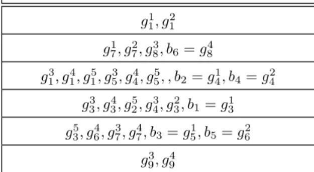
Final groups of homologous boundaries g1 1, g 2 1 g1 7, g 2 7, g 3 8, b6= g48 g3 1, g 4 1, g 5 1, g 3 5, g 4 4, g 5 5, , b2= g14, b4= g24 g3 3, g 4 3, g 5 2, g 3 4, g 2 3, b1= g13 g5 3, g 4 6, g 3 7, g 4 7, b3= g51, b5= g62 g3 9, g 4 9
Table 2 Groups of homologous boundaries obtained from groups of table 1 after add boundaries routine.
b1 b2 b3 b4 b5 b6 G1 c1 1 g1 1 g 1 7 G2 g2 1 g32 g72 c2 1 G3 g3 1 g33 g43 g53 g37 g83 g93 c3 1 G4 g4 1 g 4 3 g 4 4 g 4 6 g 4 7 g 4 9 c4 1 c 4 2 G5 g5 1 g52 g53 g55 c5 1 c52 b b b b b b b b b b b b b b b b b b b b b b b b b b b b b b b b b b b b b
Figure 3 New gene boundaries {b1, .., b6} added for the example from figure 1.
Boundaries connected by edges represent homologous boundaries. The dashed edges show the homology between the new boundaries and those originally present.
interval orientation is positive; if not, then it is negative. The result is the set of groups of homologous genomic segments.
Finally, to obtain synteny blocks for the N genomes under study, these groups are filtered in order to keep only those that contain at least one segment per genome. Final synteny blocks for the example of figure 1 are shown in figure 4.
b1 b2 b3 b4 b5 G1 c1 1 G2 g2 3 c2 1 G3 g3 1 g33 g35 g37 c3 1 G4 g4 1 g34 g44 g64 c4 1 c42 G5 g5 1 g 5 2 g 5 3 g 5 5 c5 1 c 5 2 b b b b b b b b b b b b b b b b b b b b b b b b
Figure 4 Final syntenic blocks for the example from figure 1. Genomic segment (g3 4, g 3 5) is excluded in favour of (g 3 1, g 3
3) because the latter is larger. Genomic
segments (g1 1, .., g 1 3), (g 2 1, .., g 2 3), (g 1 5, .., g 1 7), (g 2 6, g 2 7), (g 3 7, .., g 3 9), (g 4 7, .., g 4 9) are
also excluded, since they do not participate in synteny blocks for all of the considered genomes (i.e there are no segments homologous to them in certain genome(s)).
Moreover, additional filters make it possible to adapt obtained synteny blocks as common markers used in the elaboration of signed permutations in order to study rearrangement events.
2.4.1 Duplications
Generally, the permutation model does not allow duplication events, so the SyDiG algorithm proposes to keep only the longest segment in a synteny block where more than one segment belongs to one genome. The intuition behind this filter parameter is that the longer the segment, the smaller the probability that synteny was computed by chance. Nevertheless, other parameters to choose between duplicate segments should be considered such as for example synteny block neighboring. This is the subject of future work.
2.4.2 Concatenation
In the same permutation model, identifiers represent synteny blocks. Under the parsimony criterion, two identifiers that are adjacent in all the considered genomes cannot be separated to be joined again later. That is why, two modes are implemented in SyDiG algorithm. The first one provides all the synteny blocks and permits one to study their respective genomic segments. The second mode consists in concatenating synteny blocks that appear consecutively in all the
considered genomes. This leads to the construction of signed permutations with fewer identifiers, but encoding exactly the same information as far as a study of rearrangements is concerned.
2.5 Complexity
The SyDiG algorithm determines synteny blocks by constructing synteny graph and performing operations on this graph. Synteny graph construction is linear in the number of genes involved in genomic segments participating in multiplicons. Moreover, computing extended segments in the particular subgraph of the synteny graph induced by black edges can be computed in linear time in terms of the number of vertices. Finding groups of homologous genes and groups of homologous boundaries can be computed in both cases in linear time in terms of the number of vertices and dashed edges. Boundaries addition is computed in O(n3
) in the worst case, where n denotes the number of vertices in the synteny graph. Finally, the reconstruction of synteny blocks is realized by scanning the extended segments and the groups of homologous boundaries: the complexity in time is thus O(n2). Thus,
SyDiG algorithm can be computed in a simple way in O(n3) where n denotes the
number of genes involved in genomic segments.
3 Applications
3.1 GRIMM-Synteny versus SyDiG algorithm
In order to realize this comparison, we re-implemented GRIMM-Synteny as the software is not publicly available. Our reimplementation was validated using back-to-back comparison with results available on the author’s webpage (Tesler, 2004). The considerable challenge for comparing the behavior of these algorithms is the judicious choice of data processing. Indeed, GRIMM-Synteny and SyDiG rely on different data. The former proceeds by direct sequence alignment at DNA level (cleaned up by RepeatMasker (Smit et al., 2004)). The latter relies on the existence of pre-computed protein families. While DNA alignments such as BLASTZ are reasonable for closely related genomes such as mammals, only alignments at protein level can recover distant similarities for species such as yeasts (Dujon, 2006). The data presented below was retrieved from public databases on the 17th of June 2008.
- Mammal genomes human, mouse and rat, for which two sets of data were retrieved from Ensembl (release 49) and Uniprot (UniRef50, release 13.5, the 10th of june 2008) data.
- Yeast genomes Ashbya gossypii (Ergo), Kluyveromyces lactis (Klla), Kluyveromyces thermotolerans (Klth), Zygosaccharomyces rouxii (Zyro), and Saccharomyces kluyveri (Sakl), data provided by the G´enolevures Consortium (Sherman et al., 2009).
3.1.1 Yeast results
In order to apply Grimm-synteny to yeast data, we have computed 3 data sets from TBLASTX alignments: (1) unrefined alignments (206191 alignments), (2) the longest alignments when several ones overlap (51085 alignments), (3) the shortest alignments when several ones overlap (59028 alignments).
Anchors were computed by GRIMM-Anchor for the levels from 2 to 5. Results for levels 2 to 4 are shown for each data set in supplementary materials (see supplementary tables S1, S2 and S3). No 5-level anchors are found for unrefined and longest sets and only one 5-way anchor is found for the shortest set. Based on these results it was not possible to run GRIMM-Synteny and uncover synteny blocks, since the number of anchors is unsufficient.
From orthology and synteny relations identified using G´enolevures protein families (Nikolski and Sherman, 2007), SyDiG was used to compute synteny blocks for the same species. Numbers of synteny blocks for respectively two, three and four organisms are shown in supplementary materials (see supplementary tables S1, S2 and S3). A total of 640 synteny blocks are defined for the set of the 5 genomes (without concatenation). As can be noted from figure 5 (A), the number of anchors obtained for any dataset (unrefined, longest and shortest) goes dramatically down as the number of genomes increases. The comparison between multiplicons and synteny blocks on figure 5 (B) shows that the number of synteny blocks obtained by SyDiG slightly grows with each added genome while it is not the case for the multiplicons. The reason for this when going from n to n + 1 genomes, is the splitting of certain synteny blocks.
We tried to determine weather results computed by the SyDiG algorithm detect true synteny or not. In order to do this, we performed the synteny block computation on random genome data. The data were generated as follows. Each random genome set contains 5 genomes. Each of these genomes is generated starting from the complete set of the loci from one of the yeast genomes, say L∈ {Klla, Ergo, Zyro, Sakl, Klth}. First, a random number of chromosomes c between 1 and 8 is generated. Second, the number ni of loci to belong to each of
the c chromosomes is generated randomly so thatPci=1ni= n where n = |L|. Each
set of ni loci is then chosen randomly from L to be placed on the corresponding
chromosome. Finally, the orientation (positive or negative) of each locus is also chosen randomly. In total we have generated 1000 random sets of 5 genomes. The pre-processing step that consists in computing level 2 multiplicons by i-ADHoRE and using exactly the same parameters as for the real yeast data, has yeilded no synteny signal whatsoever.
3.1.2 Mammal results
Results for GRIMM-Synteny are available on the webpage ”Human-mouse-rat alignments” (by Glenn Tesler, the 16th of March 2004) (Tesler, 2004). In order to run SyDiG on the mammalian genome data, an approximation of protein families is required. We have considered two different sets:
1. the Ensembl mcl clustering results (pairwise homology relationships and gene ordered lists) (Hubbard et al., 2007),
Figure 5 A. Mean and standard deviation of number of anchors in red (black, yellow, respectively) for the unrefined (longest, shortest, respectively) dataset, of multiplicons (blue) and of synteny blocks (cyan) as a function of number of genomes. B. Zoom on mean and standard deviation of number of multiplicons (blue) and synteny blocks (cyan) as a function of number of genomes.
2. the UniRef50 clusters (pairwise homology relationships and gene ordered lists) (Consortium, 2008).
In order to be coherent with the results obtained in (Bourque and Pevzner, 2002), we have chosen the following i-ADHoRe parameters: a gap size of 15, a
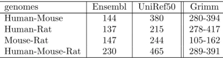
cluster gap size of 20 and 9 as minimum number of anchor points. The number of synteny blocks obtained by the SyDiG algorithm is shown in table 3 for each set of data.
genomes Ensembl UniRef50 Grimm
Human-Mouse 144 380 280-394
Human-Rat 137 215 278-417
Mouse-Rat 147 244 105-162
Human-Mouse-Rat 230 465 289-391
Table 3 Synteny blocks for mammalian genomes obtained by SyDiG algorithm based on two datasets (Esembl and UniRef50) compared to those obtained by Grimm-Synteny (see (Bourque et al., 2004)) algorithm
3.1.3 Discussion
The two methods studied here identify very similar number of synteny blocks for mammalian genomes. However, the number of anchors for yeast genomes obtained by GRIMM-synteny is very low compared to the number of alignments, and moreover the signal within genomes is lost bit by bit when the number of considered genomes increases: with as few as five yeast genomes, no anchors are found.
The main issue boils down to the observation that homologous genes correspond neither to DNA alignments, nor to anchors of level 2. Indeed, two anchors of level 2 cannot consist of the same nucleotide sequences from the same genome. Quite to the contrary, one gene from one genome Gi can be homologous
to 2 (or indeed many more) genes in another genome Gj (see figure 6).
Analysis of these results shows that for mammalian genomes SyDiG performs comparably to Grimm-Synteny. While the two data sets (UniRef50 and Ensembl) generate slightly different results, they are both comparable (for appropriately-chosen i-ADHoRe parameters) with the results published in (Bourque et al., 2004). However, when dealing with distant species such as yeasts, GRIMM-Synteny performs quite poorly. The only way to coax out any kind of signal was to perform quite strong alignment pre-filtering of the TBLASTX result.
A particularly acute problem is that the GRIMM-Synteny procedure discards n-ary homologies. Not only do these paralogous families contain biologically pertinent information, they are often the best candidates for conserved markers between genomes: in the yeasts, for example, half of the genes conserved between species are members of paralogous families of up to 30 members, and discarding these homologies can lead to drastic under-identification of chromosomal homology.
3.2 I-ADHoRe versus SydiG algorithm
3.2.1 Yeast results
We compared the i-ADHoRe method and the SyDiG algorithm on the same five species of yeasts previously presented in section 3.1. Multiplicons and synteny
Figure 6 Difference between anchors and homologous genes. We have gene homologies between (g1, g7), (g2, g7), (g3, g8), (g4, g9), (g5, g10), (g6, g11).
However, (SI1, SI7) and (SI2, SI7) can not correspond to any anchor since
SI7 is common to two couples. Other couples (SI3, SI8), (SI4, SI9),
(SI5, SI10), (SI6, SI11) represent anchors.
blocks from SyDiG were computed for the levels 2 to 5 (see supplementary tables S1,S2, S3 for respectively two, three and four organisms). We found 136 of 5-level multiplicons i-ADHoRe compared to 640 synteny blocks (without concatenation) with SyDiG.
3.2.2 Discussion
Since our SyDiG algorithm starts with the ADHoRe multiplicons of level 2, the number of multiplicons and synteny blocks obtained by the i-ADHoRe routine and the SyDiG algorithm respectively are equivalent for the pairwise comparison of species. However, profile integration for higher levels leads to a low number of multiplicons for the majority of genome triplets and quadruplets, while SyDiG uncovers homologies by considering all of the available the information. In fact, on average i-ADHoRe obtains 26.4 multiplicons of level 3 (46.6 multiplicons of level 4, respectively) compared to 431.8 synteny blocks level 3 (551.2 synteny blocks level 4, respectively) for SyDiG algorithm. For the case of 5 genomes, i-ADHoRe finds 136 multiplicons. Profiles constructed from lower levels lead to an important number of 5-level multiplicons compared to those of levels 3 and 4. However, SyDiG finds more than 600 synteny blocks for all of the 5 genomes.
3.3 Application to yeast genomes
We have applied the SyDiG algorithm in the context of the G´enolevures project (Dujon et al., 2004) for the case of non-WGD Hemiascomycetous yeasts. The data consists in 5 completely sequenced protoploid yeasts from the Saccharomycetacae clades: Kluyveromyces lactis (Klla), Saccharomyces kluyveri (Sakl), Zygosaccharomyces rouxii (Zyro), Ashbya (Eremothecium) gossypii (Ergo)
and Kluyveromyces thermotolerans (Klth). These genomes have little genome redundancy and a relatively high (for yeasts) conservation of synteny.
From orthology and synteny relations identified using G´enolevures protein families (Nikolski and Sherman, 2007), the SyDiG algorithm obtains 487 synteny blocks for these genomes (mean size 51 genes). These syntenic blocks contain 8–200 genes and cover roughly 60% of each genome. Basing these permutations only on protein-coding genes is sufficient, since yeast genomes are highly compact (protein-coding genes cover approximately 80% of the genome), and gene relics are quite rare (approximately 4%) (Dujon, 2006). For frequency distribution of synteny blocks. please refer to (Dujon et al., 2009).
By combining pairwise syntenies, each genome was factored into a sequence of ordered syntenic blocks, from which a set of distinct blocks common to all genomes was determined. An arbitrary reference genome was chosen, and all the blocks forming this genome were numbered by unique sequential identifiers from 1 to n. By keeping the longest blocks, permutations of 120 identifiers are constructed, that are representative of the pairwise evolutionary distances for these genomes. We are able to place active and inactive centromeres in each genome permutation by locating the flanking genes. Each of 9 centromeres is encoded by two identifiers, resulting in 15 additional blocks. Thus, each genome is represented as a signed permutation of 135 elements, in which chromosomal rearrangements (fusion, fission, translocation, inversion) can be studied (see (Jean et al., 2009)).
A high degree of synteny, and a limited number of large-scale rearrangements, is observed between K. thermotolerans and S. Kluyveri; they share many common adjacencies and their rearrangement distance is half of that seen between other pairs of genomes. Note that K. lactis presents two syntenic breaks in centromere areas: the centromere of Klla0F is located between the flanking genes of centromeres h and b, and the centromere of Klla0A is located between the flanking genes of centromeres h and e. Moreover, S. kluyveri has an active centromere (the centromere i), that was disabled in all the other studied genomes.
Acknowledgement
This work was done as part of the the G´enolevures Consortium. The authors thank all the members of the Consortium for numerous, friendly and creative discussions, and in particular David Sherman for running the i-ADHoRe software. The funding for this work was provided by the French National center for Scientific Research (CNRS) (GDR 2354).
References
G. Jean, D. Sherman, and M. Nikolski. Super-blocks or mining the semantics of ancestral genome architectures. JCB. accepted for publication.
Aury, J.M., Jaillon, O., Duret, L., Noel, B. et al.. Global trends of whole-genome duplications revealed by the ciliate Paramecium tetraurelia. Nature, 444(7116), 171–8.
Bourque, G. and Pevzner, P. (2002). Genome-Scale Evolution: Reconstructing Gene Orders in the Ancestral Species. Genome Research, 12, 26–36.
Bourque, G., Pevzner, P., and Tesler, G. (2004). Reconstructing the genomic architecture of ancestral mammals: Lessons from human, mouse and rat genomes. Genome Research.
Bourque, G., Zdobnov, E., Bork, P., Pevzner, P., and Tesler, G. (2005). Comparative architectures of mammalian and chicken genomes reveal highly variable rates of genomic rearrangements across different lineages. Genome Research, 15(1), 98–110.
Consortium, T. U. (2008). The Universal Protein Resource (UniProt). Nucleic Acids Research Database Issue.
Dujon, B. (2006). Yeasts illustrate the molecular mechanisms of eukaryotic genome evolution. Trends in Genetics, 22, 375–387.
Dujon, B., Sherman, D., et al. (2004). Genome evolution in yeasts. Nature, 430(6995), 35–44.
Enright, A., Dongen, S. V., and Ouzounis, C. (2002). An efficient algorithm for large-scale detection of protein families. Nucleic Acids Res., 30, 1575–1584. Hannenhalli, S. and Pevzner, P. (1995). Transforming cabbage into turnip
(polynomial algorithm for sorting signed permutations by reversals). Proceedings of twenty-Seventh Annual ACM Symposium on Theory of Computing, pages 178– 189.
Hubbard, T., Aken, B., Beal, K., Ballester, B., Caccamo, M., Chen, Y., Clarke, L., Coates, G., Cunningham, F., Cutts, T., et al. (2007). Ensembl 2007. Nucleic Acids Res., 35, Database issue, D610–D617.
Jaillon, O., Aury, J.M., Brunet, F. et al.. Genome duplication in the teleost fish Tetraodon nigroviridis reveals the early vertebrate proto-karyotype.. Nature, 431(7011), 946–¡57.
Kent, W., Baertsch, R., Hinrichs, A., Miller, W., and Haussler, D. (2004). Evolution’s cauldron: Duplication, deletion and rearrangement in the mouse and human genomes. Proc. Nat. Acad. Sci., 100(20), 11484–9.
Ma, J., Zhang, L., Suh, B., Raney, B., Burhans, R., Kent, W., and Blanchette, M. (2006). Reconstructing Contiguous Regions of an Ancestral Genome. Genome Research, 16(12), 1557–1565.
Nadeau, J. and Taylor, B. (1984). Lengths of Chromosomal Segments Conserved since Divergence of Man and Mouse. Proceedings of the National Academy of Sciences of the United States of America, Vol. 81, No. 3, [Part 1: Biological Sciences] , pages 814–818.
Nikolski, M. and Sherman, D. (2007). Family relationships: should consensus reign? - consensus clustering for protein families. Bioinformatics, 23(2), 71–76.
Pevzner, P. and Tesler, G. (2003a). Genome rearrangements in mammalian evolution: Lessons from human and mouse genomes. Genome Research.
Pevzner, P. and Tesler, G. (2003b). Human and mouse genomic sequences reveal extensive breakpoint reuse in mammalian evolution. PNAS , 100(13), 7672– 7677.
Schwartz, S., Kent, W., Smit, A., Zhang, Z., Baertsch, R., Hardison, R., Haussler, D., and W, W. M. (2004). Human-mouse alignments with BLASTZ. Genome Res., 14(4).
Simillion, C., Vandepoele, K., Saeys, Y., and Peer, Y. (2004). Building genomic profiles for uncovering segmental homology in the twilight zone. Genome Res., 14(6), 1095–106.
Simillion, C., Janssens, K., Sterck, L., and Van de Peer, Y. (2008). i-ADHoRe 2.0: An improved tool to detect degenerated genomic homology using genomic profiles. Bioinformatics, 24, 127–8.
Smit, A., Hubley, R., and Green, P. (1996-2004). RepeatMasker open-3.0. http: //www.repeatmasker.org.
Tesler, G. (2002). GRIMM: genome rearrangements web server. Bioinformatics, 18(3), 492–493.
Tesler, G. (2004). Human-mouse-rat alignments. http://nbcr.sdsc.edu/GRIMM/ HMR Aug2003/.
Trinh, P., Mclysaght, A., and Sankoff, D. (2004). Genomic features in the breakpoint regions between syntenic blocks. Bioinformatics, 20(1), 318–325. Vandepoele, K., Saeys, Y., Simillion, C., Raes, J., and Van de Peer, Y. (2002). The
Automatic Detection of Homologous Regions (ADHoRe) and Its Application to Microcolinearity Between Arabidopsis and Rice. Genome Research, 12(11), 1792–1801.
Viacheslav N. Bolshakov, Pantelis Topalis, Claudia Blass, Elena Kokoza, Alessandra della Torre, Fotis C. Kafatos, and Christos Louis. A comparative genomic analysis of two distant diptera, the fruit fly, drosophila melanogaster, and the malaria mosquito, anopheles gambiae. Genome Research, 12:57–66, 2002.
David Sherman, Tiphaine Martin, Macha Nikolski, Cyril Cayla, Jean-Luc Souciet, and Pascal Durrens. G´enolevures: protein families and synteny among complete hemiascomycetous yeast proteomes and genomes. Nucleic Acids Research, 37(Database-Issue):550–554, 2009.
The Genolevures Consortium. Comparative genomics of protoploid Saccharomycetaceae. Genome Research, 19:1967–1709, 2009.
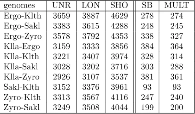
genomes UNR LON SHO SB MULT Ergo-Klth 3659 3887 4629 278 274 Ergo-Sakl 3383 3615 4288 248 245 Ergo-Zyro 3578 3792 4353 338 327 Klla-Ergo 3159 3333 3856 384 364 Klla-Klth 3221 3407 3974 328 314 Klla-Sakl 3028 3202 3716 303 288 Klla-Zyro 2926 3107 3537 381 361 Sakl-Klth 3152 3376 3961 93 93 Zyro-Klth 3313 3567 4116 247 240 Zyro-Sakl 3249 3508 4044 199 200
Table S1 Number of 2-level anchors (unrefined (UNR), longest (LON) and shortest (SHO) datasets), synteny blocks (SB) and multiplicons (MULT) on
Hemiascomycete yeasts obtained by GRIMM-Synteny, SyDiG and i-ADHoRe, respectively.
genomes UNR LON SHO SB MULT
Ergo-Sakl-Klth 174 184 440 324 63 Ergo-Zyro-Klth 214 202 441 439 5 Ergo-Zyro-Sakl 104 103 262 405 17 Klla-Ergo-Klth 320 181 353 490 8 Klla-Ergo-Sakl 348 211 387 484 8 Klla-Ergo-Zyro 314 162 345 554 2 Klla-Sakl-Klth 47 82 156 386 61 Klla-Zyro-Klth 112 87 170 480 1 Klla-Zyro-Sakl 98 124 296 472 16 Zyro-Sakl-Klth 89 187 247 284 83
Table S2 Number of 3-level anchors (unrefined (UNR), longest (LON) and shortest (SHO) datasets), synteny blocks (SB) and multiplicons (MULT) on
Hemiascomycete yeasts obtained by GRIMM-Synteny, SyDiG and i-ADHoRe, respectively.
genomes UNR LON SHO SB MULT Ergo-Zyro-Sakl-Klth 0 0 14 465 83 Klla-Ergo-Sakl-Klth 4 4 20 542 63 Klla-Ergo-Zyro-Klth 17 3 21 619 6 Klla-Ergo-Zyro-Sakl 11 1 24 604 10 Klla-Zyro-Sakl-Klth 1 3 12 526 71
Table S3 Number of 4-level anchors (unrefined (UNR), longest (LON) and shortest (SHO) datasets), synteny blocks (SB) and multiplicons (MULT) on
Hemiascomycete yeasts obtained by GRIMM-Synteny, SyDiG and i-ADHoRe, respectively.