HAL Id: hal-02111420
https://hal.archives-ouvertes.fr/hal-02111420
Submitted on 21 Oct 2019
HAL is a multi-disciplinary open access
archive for the deposit and dissemination of
sci-entific research documents, whether they are
pub-lished or not. The documents may come from
teaching and research institutions in France or
abroad, or from public or private research centers.
L’archive ouverte pluridisciplinaire HAL, est
destinée au dépôt et à la diffusion de documents
scientifiques de niveau recherche, publiés ou non,
émanant des établissements d’enseignement et de
recherche français ou étrangers, des laboratoires
publics ou privés.
Numerical investigation on evolving failure of caisson
foundation in sand using the combined Lagrangian-SPH
method
Zhuang Jin, Zhen-Yu Yin, Panagiotis Kotronis, Yin-Fu Jin
To cite this version:
Zhuang Jin, Zhen-Yu Yin, Panagiotis Kotronis, Yin-Fu Jin. Numerical investigation on evolving failure
of caisson foundation in sand using the combined Lagrangian-SPH method. Marine Georesources and
Geotechnology, Taylor & Francis, 2018, 37 (1), pp.23-35. �10.1080/1064119X.2018.1425311�.
�hal-02111420�
Numerical investigation on evolving failure of caisson foundation in sand
using the combined Lagrangian-SPH method
Zhuang Jina, Zhen-Yu Yina,b, Panagiotis Kotronisa, and Yin-Fu Jina,b
aUMR CNRS 6183, Ecole Centrale de Nantes, Research Institute of Civil Engineering and Mechanics (GeM), Nantes, France; bDepartment of Civil and
Environmental Engineering, The Hong Kong Polytechnic University, Hong Kong
ABSTRACT
Caisson foundations are often used in offshore engineering. However, for an optimum design understanding the failure process of a caisson during its installation and the subsequent external loadings is crucial. This paper focuses on the evolving failure of a caisson foundation in sand by advanced numerical modeling. A combined Lagrangian-smoothed particle hydrodynamics method is adopted to deal with the large deformation analysis. The method with parameters are first calibrated and validated by a simulation of cone penetration test in sand. The results of an experimental campaign of a caisson in the same sand are selected and validated for the numerical model. Then, more representative loading combinations are designated for numerical modeling of failure process and mode. Furthermore, three additional caisson dimensions D/d ¼ 0.5, 1.5, and 2.0 (changing the ratio of caisson diameter D to skirt length d while keeping the same soil-structure surface contact area) are simulated under six representative combined loading paths. Based on that, the influence of caisson dimension to the failure process and mode is investigated. All results are helpful to estimate all possible sliding surfaces under different monotonic combined loading paths for further limit analysis.
Introduction
A caisson is a closed-top steel tube, which is first lowered to the seafloor allowing bottom sediments to penetrate under its own weight, and then pushed to full depth with suction force produced by pumping water out of its interior. The main advantages of caissons are the convenient method of installation, their repeated use and the fact that they may mobilize a significant amount of passive suction during uplift. Recently, caissons have been widely used for different types of construction, such as gravity platform jackets, jack- ups, offshore wind turbines, subsea systems and seabed protection structures. For an optimum design, understanding the performance of the caisson foundation is however necessary.
Extensive experimental field tests on small-scale and full- scale caisson foundations have been also conducted to determine the installation characteristics and the lateral load suction foundation capacity (Hogervorst 1980; Tjelta, Guttormsen, and Hermstad 1986; Tjelta 1995). Field tests are valuable as they help to obtain necessary data for the foundation design, nevertheless they are expensive and time consuming. For these reasons, model laboratory tests have also been conducted under controlled experimental conditions either in clay (Houlsby et al. 2005; Villalobos, Byrne, and Houlsby 2010; Barari and Ibsen 2012) or sand (Huxtable et al. 2006; Cox et al. 2013; Foglia and Ibsen 2013; Zhu,
Byrne, and Houlsby 2013). Finally, 2D and 3D numerical stu-dies have been performed (Erbrich and Tjelta 1999; Sukumaran et al. 1999; El-Gharbawy and Olson 2000; Deng and Carter 2002) to study the foundation bearing capacity under different loading combinations and drainage conditions. Unfortunately, in all these numerical studies the installation process was ignored, and the evolving failure and the final failure mode under different loading combinations were not discussed.
Therefore, this paper focuses on the investigation of failure process and mode of a caisson foundation in sand by numeri-cal modeling. As the evolving failure is with large deformation, a combined Lagrangian-smoothed particle hydrodynamics method (SPH) is adopted for simulations. The method with parameters is first calibrated and validated by a simulation of cone penetration test (CPT) in sand. Then, an experimental campaign of a caisson in the same sand was selected and vali-dated for the numerical model. Then, more representative loading combinations are designated for numerical modeling of failure process and mode. Furthermore, three additional caisson dimensions D/d ¼ 0.5, 1.5, and 2.0 (changing the ratio of caisson diameter D to skirt length d while keeping the same soil-structure surface contact area) are simulated under six representative combined loading paths. Based on that, the influence of caisson dimension to the failure process and mode is investigated.
SPH based modeling approach
SPH method and combined Lagrangian-SPH technique The smooth particle hydrodynamics method was first developed by Gingold and Monaghan (1977) for simulations in astrophysics. Further developments of the method allowed for applications to a broad range of problems in solid mechanics. In SPH simulations, the computational domain is discretized into a finite number of particles, each representing a certain volume and mass of material (fluid or solid) and carrying simulation parameters such as acceleration, velocity, density, and pressure/stress.
The material properties f(x)at any point x in the simulation domain are then calculated according to an interpolation pro-cess over its neighboring particles that are within an influence domain Ω through
f xð Þ ¼ Z
X
f xð ÞW x0 ð x0; hÞdx0 ð1Þ where W is the kernel or smoothing function, which is essentially a weighting function.
The continuous integral representation of the field variable f(x)in Eq. (1) can be further approximated by the summation over neighboring particles as
f xð Þ ¼X N i¼1 f xð ÞW xi ð xi; hÞVi ¼X N i¼1 f xð ÞW xi ð xi; hÞ mi qi ð2Þ
where Vi, mi, and qi are the volume, mass and density of the
ith particle, respectively; and N is the number of particles within the influence domain. The spatial derivative of field variable f(x) can be approximated through the differential operations on the kernel function
@f xð Þ @x ¼ XN i¼1 mi qif xð Þi @W xð xi; hÞ @xi ð3Þ
It is indicated by Eq. (1) through Eq. (3) that the efficiency and accuracy of SPH simulations depend on the kernel func-tion. The SPH particles are used as interpolation points and are the basis for calculating all the field variables in the continuum around them. The SPH particles, like the objects in astrophysics, can be separated by a large distance. The field variables between the SPH particles are approximated (smoothed) by the smoothing shape functions. The interaction between SPH particles starts when a particle gets to a certain distance (smoothing length h) from another one. SPH particles interact with each other only if they are within the influence domain. Otherwise, they are independent from each other. Therefore, larger smoothing length (i.e., larger influence domain) generally results in a smoother or more continuous behavior as the SPH particles are more interdependent with each other; whereas smaller smoothing length (i.e., smaller influence domain) generally yields more discrete behaviors as the SPH particles are more independent from each other. In a solid body, discretized with densely packed SPH particles there is still no connectivity defined between the particles through the
mesh. A major attraction of the SPH technique is that the need for a fixed computational grid is removed when calculating spatial derivatives. Instead, estimates of derivatives are obtained from analytical expressions based on the derivatives of the smoothing functions (Li and Liu 2002). Since the connectivity between the particles is generated as a part of the computation and can change over the time, the SPH method can handle analysis of very large deformations and displacements.
However, one disadvantage of the SPH method over the Lagrangian method is their computational demand (Bojanowski 2014). The SPH method is also less accurate under small deformations. For this reason, only a part of the soil domain can be modeled by the SPH method, and a Lagrangian model can be adopted for the rest, which is the so-called combined Lagrangian-SPH technique. In this study, the combined Lagrangian-SPH technique provided by the commercial finite element code ABAQUS was adopted. The function “Tie Constraint” was adopted to treat the interface of SPH domain and Lagrangian domain so that no relative motion exists. It allows fusing two domains even though their meshes are not identical. More detailed can be found in ABAQUS manual (Hibbitt, Karlsson, and Sorensen 2013). Combined Lagrangian–SPH model
Selected experimental campaign
The first task of the study is to calibrate a numerical model according to experiments, based on which the failure process and mode can be further investigated. For this purpose, a well-documented series of laboratory tests of caisson foundation in sand including the installation phase and the application of monotonic loadings by Foglia et al. (2015) was selected. The experimental set-up consists of a sand box (1,600 � 1,600 � 1,150 mm), a loading frame and a hinged beam. A system of steel cables and pulleys induces loadings to the foun-dation through an electric motor drive placed on the hinged beam. The load, set by three weight hangers, is transferred to the foundation through a vertical beam bolted on the caisson lid. The foundation is instrumented with three linear variable differential transformer (LVDTs) and two load cells. A CPT was first performed to assess the soil parameters. The caisson foundation is made of steel, with an outer diameter of 300 mm, a lid thickness of 11.5 mm, a skirt length of 300 mm and a skirt thickness of 1.5 mm. Six tests of caisson foundation were performed under different monotonic loading combina-tions (one pure vertical load up to failure and five different dimensionally homogeneous moment to horizontal load ratios (M/DH ¼ 1.1, 1.987, 3.01, 5.82, and 8.748) at constant vertical load).
Numerical model
The whole finite element model was created with the same dimension as the experimental box. On the lateral sides, the horizontal displacements are constrained, and on the bottom face the translational degrees of freedom with all displace-ments are constrained. For modeling the soil, the perfect elastoplastic model Mohr–Coulomb was adopted in this study. The constitutive equations are presented in Appendix. Model parameters can be achieved using optimization (Jin et al. 2016,
2017) based on the test results by Ibsen et al. (2009) and presented as follows: the Young modulus E is 26 MPa, the Poisson ratio υ is 0.25, the frictional angle ϕ is 40.8°, the dilation angle ψ is 17.5°, and the cohesion c is 6 kPa. Further-more, the density is 1,100 kg/m3, the friction coefficient of the
soil-caisson interface is 0.35 (k ¼ tan(ϕ/2)) and the damping ratio is set to 0.
In the combined Lagrangian-SPH model, only the portion of the soil experiencing the large deformation is modeled with SPH particles (Figure 1). The SPH domain is a length of 1,400 mm at the side with horizontal or moment loading, a width of 800 mm at the other side, a height of 1,150 mm up to the bottom, with a total number of 88,407 particles. The outside Lagrangian mesh is composed by 1,05,984 hexahedral elements. For the model with densely packed SPH particles, the initial particle distance in each direction stays approxi-mately constant to be homogenous. The calculation domain modeled with particles (SPH domain) can interact with the Lagrangian finite element via contact (Hibbitt, Karlsson, and Sorensen 2013). The contact interaction is the same as any contact interaction between a node-based surface (associated with the particles) and an element-based or analytical surface. Both general contact and contact pairs can be used. All interaction types and formulations available for contact involving a node-based surface are allowed, including cohesive behavior. Different contact properties can be assigned through the usual options (Hibbitt, Karlsson, and Sorensen 2013). For the reason of numerical stability, at least four SPH particles per face of a Lagrangian element in contact are considered.
The caisson was modeled using 927 rigid tetrahedron ele-ments with the same dimension and thickness as experiment. According to Foglia et al. (2015), the density of the caisson is taken equal to 7,800 kg/m3, the Young modulus 200 GPa and
the Poisson ratio 0.3. The caisson was initially positioned on the surface of soil at the center of box. For the simulation of CPT, the caisson was replaced by a cylinder bar (using 807 rigid tetrahedron elements) with a diameter of 20 mm and a 60° cone at bottom according to Foglia et al. (2015).
In SPH method, each particle represents one gauss integration point. Accordingly, similarly to the element in FEM, the total strain of each particle is composed of elastic
and plastic parts when using the MC model in SPH. In this study, the equivalent plastic strain PEEQ defined as PEEQ ¼ ffiffiffiffiffiffiffiffiffiffiffiffiffiffiffiffiffiffiffiffiffiffiffiffiffiffiffiffiffiffi2 23= 3 _epij:_e
p ij
� � r
(where _ep
ij is the tensor of plastic
strain rate) was used to describe the plastic deformation. Model calibration for CPT
To validate the combined Lagrangian-SPH model with material parameters, a CPT simulation was first performed. During the simulation, the velocity of cone penetration was equal to 5 mm/s according to Foglia et al. (2015). A rigid Mohr–Coulomb type interface model was adopted with a typical soil-structure interface friction coefficient assumed for the simulation. The interface model was applied on the entire (tip and shaft) surface of the cone.
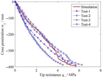
The comparison between experimental and numerical results is presented in Figure 2, where four CPT experimental results are provided by Foglia et al. (2015). A good agreement was achieved which reveals that the combined Lagrangian- SPH model with material parameters are therefore acceptable, and can be continued for caisson foundations.
Figure 1. Combined Lagrangian-SPH model: (a) in 3D, and (b) for middle cross section.
Figure 2. Comparison between experiments and simulation of CPT for tip
The fields of equivalent plastic strain (PEEQ, same as deviatoric plastic strain), deviatoric stress (S Mises, Pa), and mean effective stress (S Pressure, Pa) corresponding to a penetration of 400 mm are plotted in Figure 3, which shows reasonable distributions of these terms due to the cone penetration with an influence distance much smaller than the domain of SPH particles.
Model calibration for caisson foundation
The combined Lagrangian-SPH model of Figure 1 was used to simulate one pure penetration test by vertical displacement control at a rate of 5 mm/s, and five tests at different dimensionally homogeneous moment to horizontal load ratios (M/DH ¼ 1.1, 1.987, 3.01, 5.82, and 8.748) at a constant verti-cal load of 241N by horizontal displacement control combined with rotation control at the middle point of caisson. For the simulation using explicit method, the loading rate is usually ten times the real loading rate for saving the computational time while the quasi-static state should be simultaneously guaranteed (Qiu, Henke, and Grabe 2011). In ABAQUS/ SPH, quasi-static state is defined such that the ratio of kinematic energy over internal energy is smaller than 5%. However, it is a pity that the real loading rates were unknown in this case. Accordingly, the displacement rate of 10 mm/s and rotation rate of 0.5°/s were selected which guarantee the quasi-static state. All monotonic loading paths were followed until the vertical bearing capacity (VM) or the horizontal capacity and moment capacity (MR) are reached. The simu-lated deformations corresponding to the bearing capacities for all model tests are summarized in Table 1.
Figure 4 shows the applied vertical force versus vertical dis-placement for the pure vertical loading test. Figure 5 presents the results of five typical M/DH values (1.100, 1.987, 3.010, 5.820, and 8.748). For all five cases the horizontal load (H)
versus the horizontal displacement (U) and the dimen-sionally homogeneous moment (M/D) versus the rotational displacement (Dθ) are plotted for comparisons. Note that the calculated curves are not smooth, which is usually called numerical noise when using the SPH technique that uses the explicit time integration method. This numerical noise could be affected by various factors, such as the estimation of the stable time increment by element-by-element method, the applied contact law between pile and soil, and the application of mass scaling method for improving the calculation efficiency (Hibbitt, Karlsson, and Sorensen 2013). For all tests good agreement was achieved through comparisons between experiments and simulations. The combined Lagrangian- SPH model with material parameters was thus well calibrated, and can be used for further numerical investigations on failure process and mode.
Two extreme cases were selected to examine the domain of large deformation: one pure vertical loading test and one moment combined horizontal loading test (M/DH ¼ 8.748). The fields of equivalent plastic strain (PEEQ), deviatoric stress (S Mises, Pa) and mean effective stress (S Pressure, Pa) are plotted in Figure 6 for pure vertical loading test and for moment combined horizontal loading test. Both results show reasonable distributions of three terms due to loadings with an influence distance (large deformation domain in both
Figure 3. Results of CPT simulation: (a) field of equivalent plastic strain (PEEQ), (b) field of deviatoric stress (S Mises, Pa), and (c) field of mean effective stress
(S Pressure, Pa). Note: CPT, cone penetration test.
Table 1. Initial deformation under the capacity loadings for each case.
M/DH u(mm) Dθ(mm) HR(N) MR/D(N)
1.1 5.8 7.4 420 540
1.987 4.6 6.0 330 640
3.01 4.0 5.5 190 690
5.82 5.0 6.8 110 700
vertical and horizontal directions) much smaller than the domain of SPH particles.
In addition, the failure envelope on the H:M/D loading plane summarized by Villalobos, Byrne, and Houlsby (2010), Ibsen
et al. (2014) and Foglia et al. (2015), is plotted in Figure 7, comparing with all results obtained by simulations under the same vertical loading. Good agreement was achieved which reveals the numerical modeling in this study is appropriate.
Figure 5. Comparison between experimental vs. Numerical results for tests of monotonic multidirectional loading paths: (a, c) horizontal force versus horizontal
displacement, (b, d) dimensionally homogeneous moment versus rotational displacement.
Figure 6. Contour of plastic deviatoric strain (PEEQ), deviatoric stress (S, Mises, Pa) and Mean stress (S Pressure, Pa) for (a–c) one pure vertical loading test and (d–f)
Analysis of failure process and mode
Based on the calibrated model, various tests under different loading combinations were simulated: three single loading tests (P–V, P–H, and P–M for pure vertical, horizontal, and moment loading, respectively), four tests under two combined loadings (C–VH for horizontal and vertical loadings, C–VM for vertical loading and moment, C–H+M for horizontal loading and
moment at the same direction, C–H−M for horizontal loading
and moment in the opposite direction), and two tests under three combined loadings (C–VH+M and C–VH−M which are C–H+M
and C–H−M with additional vertical loading). During all
simula-tions, the displacement rate was kept as 10 mm/s and rotation rate 0.5°/s. The displacement or rotation angle is big enough to ensure the complete development of sliding surface in sand.
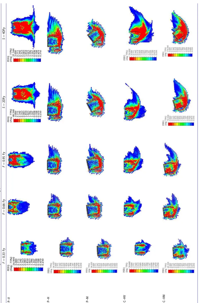
All test simulations are summarized in Table 2 for the evol-ution of sliding surface of caisson foundation represented by the equivalent plastic strain. To have a good understanding on the evolution, five moments during the loading were selected and recorded with the contour of equivalent plastic strain: at 0.33 Fy (Fy is the yield force or moment), 0.66 Fy, 0.95 Fy, 2 DFy (DFy is the displacement or rotation angle at 0.95 Fy) and 4 DFy. All test simulations are summarized in
Table 2. Thus, the evolution of sliding surface of caisson foun-dation can be clarified by five selected successive moments during the loading. Figure 8 illustrates how to determine the yield force Fy, in which softening part is not taken into account, and only the peak value is used to define the failure. Note that the definition of yield strength presented in Figure 8
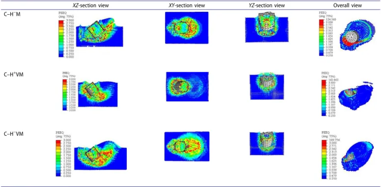
was followed by the model tests by Foglia et al. (2015). The purpose was to completely reproduce the model test by SPH simulation. Table 3 presents different views of each simulation at 4 DFy. In particular, XZ section, XY section, YZ section, and overall (3D) view are included.
Failure modes under paths of single loading
For the single vertical loading test (P–V), plastic zone expands along with vertical direction at the beginning. With increasing
displacement, the soil underneath the caisson is compressed and plastic zone expands also along with the horizontal direc-tion at the same time. High plastic zone mainly concentrates on the bottom of the caisson. The final plastic zone looks like a matrass, as shown in Table 2.
For the single horizontal loading test (P–H), as presented in
Table 2, the plastic zone expands along with the horizontal direction. Because the shear stress level at the bottom of caisson is higher than above, the plastic zone at bottom expands smaller than above layer. As a result, the final sliding surface is similar to the spheroidicity, shown in Table 3. High plastic zone mainly centralizes on sliding plane and near the right skirt of caisson.
For the single moment loading test (P–M), the plastic zone expands along with circumferential direction. Comparing with above two cases, expanded area of plastic zone is smaller. High plastic zone primarily concentrates on the sliding plane near the left inner skirt of caisson.
Failure modes under paths of two combined loadings For the case of C–VH, the plastic zone extends following the resultant force direction of H and V first, 45° with the horizontal direction. With the displacement increasing, a polarization of plastic zone occurs. As shown in Table 2, the plastic zone extends obviously along with two directions, one is horizontal and the other is vertical. High plastic zone mainly concentrates on the 45° glide plane, the area near the right skirt of caisson and the area near the bottom of caisson. Compared to the cases of pure vertical and pure horizontal loading, the plastic zone of C–VH can be considered as the superposition of the former two. Under combined loadings V and M for the case of C–VM, the plastic zone expands along with vertical and circumfer-ential directions. Compared to the case of pure moment, the extension of plastic zone along with circumference is larger in this case. The final sliding surface approximates as a sphe-roidicity. High plastic zone primarily centralizes on the sliding plane near the left inner skirt of caisson.
Table 2. Evolution of sliding surface of caisson foundation under different loading paths. F ¼ 0.33 Fy F ¼ 0.66 Fy F ¼ 0.95 Fy S ¼ 2DFy S ¼ 4DFy P–V P–H P–M C–HV C–VM (Continued )
Table 2. Continued. F ¼ 0.33 Fy F ¼ 0.66 Fy F ¼ 0.95 Fy S ¼ 2DFy S ¼ 4DFy C–H +M C–H − M C–H +VM C–H −VM
As shown in Table 2, the plastic zone expands along with circumferential and horizontal direction under combined loadings of H and M for the case of C–H+M. As mentioned
above, because the shear stress level of the upper soil layer is lower, the plastic area expands more obviously. As a result, the sliding surface looks like a basin and the plastic zone is basically bilateral symmetric. Compared to the case of pure moment, the plastic zone in this case extends more obviously at the left side. The distribution of high plastic zone is relatively discrete.
Similar to the above case, the plastic zone of C–H−M
expands along with circumferential and horizontal directions.
Figure 8. Determination of the peak values.
Table 3. Specified views of sliding surface of caisson foundation under different loading paths.
XZ-section view XY-section view YZ-section view Overall view P–V P–H P–M C–HV C–VM C–H+M (Continued)
Compared to C–H+M, because of the opposite direction of
horizontal loading, the plastic extension is more obvious in this case. The plastic extension of H and M is mutually stimulative, with a positive correlation. The high plastic area mainly centralizes on the sliding plane, presented with a continuous zone combining horizontal and circumferential extension.
Failure modes under paths of three combined loadings As shown in Table 2, the extension of plastic zone for C–H
+VM follows three directions, i.e., horizontal, vertical, and
circumferential. The final sliding surface is a shape of hemi-spheroidicity. The high plastic zone primarily concentrates on the left skirt (including inner and outer side) of caisson with the area near the caisson bottom.
For the case of C–H−VM, the edge of plastic zone presents
as the shape of smooth arc. With the rotational displacement increasing, the upper soil layer is lifted off the ground. The high plastic zone primarily concentrates on the sliding plane near the caisson bottom. Like the case of C–H−M, the
exten-sion of plastic zone due to H and M is mutually stimulative. Compared to the case of C–H−M, the final sliding surface is
smaller. The reason is that the vertical loading enhances the
interaction between the caisson and the soil, thereby reducing the displacement and rotation of the caisson.
Yield strength and sliding surface area under different loading conditions
To analyze the relationship between yield strength and sliding surface expansion under different loading conditions, the sliding surface area of each case was calculated. The shape of sliding surface of all above cases can be approximated as ellipsoid, which can be described as,
x2 a2þ y2 b2þ z2 c2¼ 1 ð4Þ where a, b, and c represent the length of three dimensions, expressed as follows:
a¼ 0:25a1þ 0:5a2þ 0:25a3 b¼ 0:25b1þ 0:5b2þ 0:25b3
c¼ 0:25c1þ 0:5c2þ 0:25c3
(
ð5Þ
To measure (a1, a2, and a3), (b1, b2, and b3), and (c1, c2, and c3),
an illustrative example was given, as shown in Figure 9. For the XZ-section, because of the irregular shape, the weights of
Table 3. Continued.
XZ-section view XY-section view YZ-section view Overall view C–H−M
C–H+VM
C–H−VM
a1, a2, and a3 for calculating a are 0.25, 0.5, and 0.25, respectively. Same method was adopted in another two directions.
By measuring the length of three dimensions for each case, the sliding surface area was calculated by following the Knud Thomsen formula, S� 4p a nbnþ ancnþ bncn 3 � �1n ð6Þ
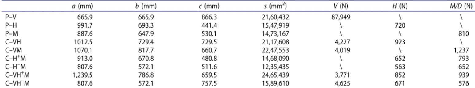
where n � 1:6075 with the relative error approximated to 1.061% (Krajcik and McLenithan 2001); The related results are summarized in Table 4. Figure 10 shows the sliding surface area under different loading conditions.
As shown in Table 4 and Figure 10, among the single loading cases, while specifying the vertical loading, the sliding surface develops more notably representing higher strength than other two pure loading conditions. The sliding surface area of pure H and M cases stays nearly the same.
For the two combined loading cases, while specifying the C–MH loadings, the sliding surface area reaches the minimum. Besides, while V combined with H or M, compared to single loading case, the global bearing capacity is improved. For the three combined loading cases, comparing the case C–VH+M to C–VH−M, when the direction of H and M keep
the same rotational direction, the sliding surface develops more obviously with the bearing capacity of H and M also being higher than the opposite one.
Influence of caisson dimension to failure progress and mode
The dimension of caisson needs to be optimized during design, for which its influence needs to be estimated. For this purpose, three additional dimensions were designated with D/d ¼ 0.5, 1.5, and 2 (D is the diameter of caisson and d is the skirt length of caisson) keeping the same soil-structure contact area: the narrow-deep caisson R0.5 (D ¼ 224 mm, d ¼ 447 mm), wide-shallow caissons R1.5 (D ¼ 350 mm, d ¼ 233 mm) and R2.0 (D ¼ 387 mm, d ¼ 193 mm). For each dimension, six representative combined loading paths were selected for simulations, as: H–V, V–M, H+–M, H−–M,
H+–V–M, H−–V–M.
Note that the failure progress and failure mode are very similar to that of D/d ¼ 1.0 only with different size of sliding surface, models with plastic zone are thus not plotted in this section. Only yield strength and sliding surface area are estimated for comparisons. As presented in Figure 11, in all six cases of specified combined loadings, with the ratio D/d increasing, the yield strength of vertical loading increases slightly and linearly, while the horizontal and moment capacities show a slightly linear decrease. Comparing figure case H+–M to H−–M, H+–V–M to H−–V–M, for the opposite
direction of applied horizontal loading, the capacities of hori-zontal force and moment present a reducing trend. Besides, when the vertical loading is applied, the capacities of H and M are improved.
Table 4. Yield strength and sliding surface area under various loading paths.
a (mm) b (mm) c (mm) s (mm2) V (N) H (N) M/D (N) P–V 665.9 665.9 866.3 21,60,432 87,949 \ \ P–H 991.7 693.3 441.4 15,47,919 \ 720 \ P–M 887.6 647.9 530.1 14,73,167 \ \ 810 C–VH 1012.5 729.4 729.5 21,17,608 4,227 923 \ C–VM 1070.1 817.7 660.7 22,47,553 4,019 \ 1,237 C–H+M 913.0 670.8 480.8 14,68,090 \ 652 793 C–H−M 807.6 572.1 511.6 12,35,435 \ 563 652 C–VH+M 1,239.5 786.8 659.5 24,65,439 3,771 852 939 C–VH−M 807.6 572.1 757.5 15,89,610 4,625 671 576
The sliding surface area was calculated for all cases, and is plotted in Figure 12. In all six cases of specified loading com-binations, with the ratio D/d increasing, the sliding surface area decreases slightly and then increases linearly. Comparing the case H+–M to H−–M, H+–V–M to H−–V–M, for the
opposite direction of applied horizontal loading, the expansion of sliding surface presents a reducing trend. Besides, when the vertical loading is applied, the sliding surface area is enlarged.
Conclusion
The evolving failure of a caisson foundation in sand was modelled under different loading combinations. A combined
Lagrangian-SPH method was adopted to deal with the large deformation analysis. The method with parameters were first calibrated and validated by a simulation of CPT in sand. The results of an experimental campaign of a caisson in the same sand were selected for simulations, based on which the numerical model with parameters was validated.
Then, more representative loading combinations were designated for numerical modeling of failure process and mode. It can be concluded that, (1) the final shape of sliding surface under different combined loadings with H or/and M is similar to each other, but with different size; (2) the vertical loading improves the horizontal strength or/and moment strength and thus reinforces generally the bearing capacity of the caisson foundation; (3) for the case with the same direction of H and M, the sliding surface develops more obviously and the bearing capacity is bigger than the case of opposite direction of H and M.
Furthermore, three additional caisson dimensions D/d ¼ 0.5, 1.5, and 2.0 (changing the ratio of caisson diameter D to skirt length d while keeping the same soil-structure surface contact area) were simulated under six representative combined loading paths. Based on that, the influence of caisson dimension to the failure process and mode was investigated.
It was found that with the ratio D/d increasing, the yield strength of vertical loading increases slightly and linearly, while the horizontal and moment capacities show a slightly linear decrease. The sliding surface area presents a trend of slightly decreasing and then increasing linearly.
All simulation results are helpful to estimate all possible sliding surfaces under different monotonic combined loading
Figure 12. Sliding surface area under specified combined loadings with
different ratio of D/d.
paths for further limit analysis. Along this line, the critical state based soil model with the real scale suction bucket foundation will be analyzed in the future.
Funding
The financial support for this research came from the National Natural Science Foundation of China (Grant No. 51579179). These supports are greatly appreciated.
References
Barari, A., and L. B. Ibsen. 2012. Undrained response of bucket foundations to moment loading. Appl. Ocean Res. 36:12–21.
doi:10.1016/j.apor.2012.01.003.
Bojanowski, C. 2014. Numerical modeling of large deformations in soil structure interaction problems using FE, EFG, SPH, and MM-ALE
formulations. Arch. Appl. Mech. 84:743–55. doi:10.1007/s00419-014-
0830-5.
Cox, J. A., S. Bhattacharya, D. Lombardi, and D. M. Wood. 2013. Dynamics of offshore wind turbines supported on two foundations.
Proc. ICE—Geotech. Eng. 166 (2):159–69. doi:10.1680/geng.11.00015
Deng, W., and J. P. Carter. 2002. A theoretical study of the vertical uplift capacity of suction caissons. Int. Soc. Offshore Polar Eng. 12 (2):342–49. El-Gharbawy, S., and R. Olson. 2000. Modeling of suction caisson foundations. The Tenth International Offshore and Polar Engineering Conference, International Society of Offshore and Polar Engineers, 28 May–2 June 2000, Seattle, Washington, USA, vol. 2, 670–77. Erbrich, C. T., and T. I. Tjelta. 1999. Installation of bucket foundations
and suction caissons in sand-geotechnical performance. Offshore
Technology Conference, 3–6 May, 1999 Houston, TX. doi:10.4043/
10990-MS.
Foglia, A., G. Gottardi, L. Govoni, and L. B. Ibsen. 2015. Modelling the drained response of bucket foundations for offshore wind turbines under general monotonic and cyclic loading. Appl. Ocean Res. 52:80–91.
Foglia, A., and L. B. Ibsen. 2013. A similitude theory for bucket foundations under monotonic horizontal load in dense sand. Geotech.
Geol. Eng. 31:133–42. doi:10.1007/s10706-012-9574-6.
Gingold, R. A., and J. J. Monaghan. 1977. Smoothed particle hydrodynamics: Theory and application to non-spherical stars. Mon.
Not. R. Astron. Soc. 181:375–89. doi:10.1093/mnras/181.3.375.
Hibbitt, K., B. Karlsson, and P. Sorensen. 2013. ABAQUS/explicit user’s
manual (version 6.14). Pawtucket, RI: Hibbitt, Karlsson & Sorensen,
Inc.
Hogervorst, J. R. 1980. Field trails with large diameter suction piles. Offshore Technology Conference, 5–8 May, 1980, Houston, TX,
217–22. doi:10.4043/3817-MS.
Houlsby, G. T., R. B. Kelly, J. Huxtable, and B. W. Byrne. 2005. Field trials of suction caissons in clay for offshore wind turbine foundations.
Géotechnique 55:287–96. doi:10.1680/geot.2005.55.4.287.
Huxtable, J., R. B. Kelly, G. T. Houlsby, and B. W. Byrne. 2006. Field trials of suction caissons in sand for offshore wind turbine foundations.
Géotechnique 56:3–10. doi:10.1680/geot.2006.56.1.3.
Ibsen, L. B., M. Hanson, T. Hjort, and M. Thaarup. 2009. Mc-parameter calibration of baskarp sand. No. 15, Department of Civil Engineering, Aalborg University, Denmark.
Ibsen, L. B., K. A. Larsen, and A. Barari. 2014. Calibration of failure criteria for bucket foundations on drained sand under general loading.
J. Geotech. Geoenviron. Eng. 140:4014033. doi:10.1061/(ASCE)GT.
1943-5606.0000995.
Jin, Y.-F., Z.-Y. Yin, S.-L. Shen, and P.-Y. Hicher. 2016. Selection of sand models and identification of parameters using an enhanced genetic
algorithm. Int. J. Numer. Anal. Methods Geomech. 40:1219–40.
doi:10.1002/nag.2487.
Jin, Y.-F., Z.-Y. Yin, S.-L. Shen, and D.-M. Zhang. 2017. A new hybrid real-coded genetic algorithm and its application to parameters identification of soils. Inverse Probl. Sci. Eng. 25:1343–66.
doi:10.1080/17415977.2016.1259315.
Krajcik, R. A., and K. D. McLenithan. 2001. Final answers. http://www.
numericana.com/answer/ellipsoid.htm#thomsen. Accepted date: 23
October, 2001.
Li, S., and W. K. Liu. 2002. Meshfree and particle methods and their applications. Appl. Mech. Rev. 55:1–34.
Qiu, G., S. Henke, and J. Grabe. 2011. Application of a coupled Eulerian– Lagrangian approach on geomechanical problems involving large deformations. Comput. Geotech. 38:30–39.
Sukumaran, B., W. O. McCarron, P. Jeanjean, and H. Abouseeda. 1999. Efficient finite element techniques for limit analysis of suction caissons under lateral loads. Comput. Geotech. 24:89–107.
Tjelta, T. I. 1995. Geotechnical experience from the installation of the Europipe jacket with bucket foundations. Offshore Technology
Conference, 1–4 May, 1995, TX. doi:10.4043/7795-MS.
Tjelta, T. I., T. R. Guttormsen, and J. Hermstad. 1986. Large-scale penetration test at a deepwater site. Offshore Technology Conference,
5–8 May, 1986, TX. doi:10.4043/5103-MS.
Villalobos, F. A., B. W. Byrne, and G. T. Houlsby. 2010. Model testing of suction caissons in clay subjected to vertical loading. Appl. Ocean Res.
32:414–24. doi:10.1016/j.apor.2010.09.002.
Zhu, B., B. W. Byrne, and G. T. Houlsby. 2013. Long-term lateral cyclic response of suction caisson foundations in sand. J. Geotech.
Geoen-viron. Eng. 139:73–83. doi:10.1061/(ASCE)GT.1943-5606.0000738.
Appendix
The basic equations of MC model in ABAQUS are presented as follows: Yield function: F¼ Rmcq ptan / c ¼ 0 ðA1Þ RmcðH; /Þ ¼ ffiffiffi1 3 p cos /sin H þ p 3 � � þ13cos H þ� p3� tan / with cos 3Hð Þ¼ J3
q � �3 ðA2Þ Potential function: G¼ ffiffiffiffiffiffiffiffiffiffiffiffiffiffiffiffiffiffiffiffiffiffiffiffiffiffiffiffiffiffiffiffiffiffiffiffiffiffiffiffiffiffiffiffi ec0tan w ð Þ2þ Rð mwqÞ2 q ptan w ðA3Þ Rmw¼ 4 1 e 2 ð Þcos2Hþ 2eð 1Þ2 2 1 e2� cos H þ 2e 1ð Þ ffiffiffiffiffiffiffiffiffiffiffiffiffiffiffiffiffiffiffiffiffiffiffiffiffiffiffiffiffiffiffiffiffiffiffiffiffiffiffiffiffiffiffiffiffiffiffiffiffiffiffiffiffiffiffiffiffi 4 1 eð 2Þ cos Hð Þ2þ 5e2 4e q Rmc p 3; / �
� with e¼ 3 sin3 þ sin //
ðA4Þ
where F is yield function, q is deviatoric stress, p is mean stress, ϕ is friction angle, c is cohesion, J3 is the third invariant
of the deviatoric strain tensor, G is potential function, ψ is dilatancy angle, c0 is the initial value of cohesion, ε ¼ 0.1 as