Using SMT Solving for the Lookup of Infeasible Paths in Binary Programs

O

pen

A

rchive

T

OULOUSE

A

rchive

O

uverte (

OATAO

)

OATAO is an open access repository that collects the work of Toulouse researchers and

makes it freely available over the web where possible.

This is an author-deposited version published in :

http://oatao.univ-toulouse.fr/

Eprints ID : 15319

The contribution was presented at WCET 2015 :

http://www.bsc.es/caos/WCET2015

To cite this version :

Ruiz, Jordy and Cassé, Hugues Using SMT Solving for the

Lookup of Infeasible Paths in Binary Programs. (2015) In: 15th International

Workshop on Worst-Case Execution Time Analysis (WCET 2015), 7 July 2015

(Lund, Sweden).

Any correspondence concerning this service should be sent to the repository

administrator:

staff-oatao@listes-diff.inp-toulouse.fr

Using SMT Solving for the Lookup of Infeasible

Paths in Binary Programs

∗

Jordy Ruiz and Hugues Cassé

Abstract

Worst-Case Execution Time (WCET) is a key component to check temporal constraints of real-time systems. WCET by static analysis provides a safe upper bound. While hardware modelling is now efficient, loss of precision stems mainly in the inclusion of infeasible execution paths in the WCET calculation. This paper proposes a new method to detect such paths based on static analysis of machine code and the feasibility test of conditions using Satisfiability Modulo Theory (SMT) solvers. The experimentation shows promising results although the expected precision was slightly lowered due to clamping operations needed to cope with complexity explosion. An important point is that the implementation has been performed in the OTAWA framework and is independent of any instruction set thanks to its semantic instructions.

1998 ACM Subject Classification J.7 Real time

Keywords and phrases WCET, infeasible paths, SMT, machine code

Digital Object Identifier 10.4230/OASIcs.WCET.2015.95

1

Introduction

Temporal properties verification is utterly important for critical embedded systems like avionics, automotive or any system involving real-time constraints. Such verification is usually performed in two steps: first, the Worst-Case Execution Time (WCET) of each task composing the system is computed and, second, this WCET is used to check if the set of tasks is schedulable according to the system real-time constraints. Hence, the WCET determination must be (a) safe (higher than the real worst-case execution) to ensure soundness of the scheduling and (b) tight or precise to minimize the hardware required to run the system.

This paper addresses the computation of WCET by static analysis that ensures safety of WCET by construction at the price of tightness: an overestimation of the WCET is produced without guaranty about precision. A successful and widely used approach to compute statically WCET is Implicit Execution Path Technique or IPET. It models the execution paths of the program and the host hardware (that induces execution time) as an Integer Linear System, ILP, whose maximization function is the estimated WCET. Lots of work has been devoted to model the hardware and, for some classes of microprocessor parts (LRU caches, pipeline, etc.), provides precise results.

Yet, modelling the execution paths seems to remain a challenge and could be an important source of precision improvement. Basically, IPET models the execution paths by a Control Flow Graph, CFG, where vertices represent blocks of instructions1_{and edges, execution flow}

between blocks. The CFG is usually derivated from a program by a basic analysis examining

∗ _{This work was partially supported by the french ANR project, W-SEPT.}

1 _{Usually machine instructions to be as close as possible to the hardware.} © Jordy Ruiz and Hugues Cassé;

licensed under Creative Commons License CC-BY

15th International Workshop on Worst-Case Execution Time Analysis (WCET 2015). Editor: Francisco J. Cazorla; pp. 95–104

OpenAccess Series in Informatics

the branch targets of control instructions. Therefore, the set of paths represented by the CFG (potentially unbounded if the program contains loops) includes (a) all actual paths of the program and (b) other paths that are infeasible because of the program internal logic.

Applying the IPET approach to the CFG model of execution paths is consistent (as long as a maximum bound is provided for loops) because it consists in computing the maximum of execution paths. Adding infeasible paths to the set of actual execution paths will, in the worst case, produce an estimated WCET higher than the actual WCET. Yet, the added execution paths may cause a loss of tightness (distance between real WCET and estimated WCET) that is difficult to evaluate. In practice, separating feasible and infeasible paths faces the complexity issue of the number of paths in the program and in the CFG.

This paper proposes a new approach to detect infeasible paths in machine language programs based on (a) the representation of program states as labelled sets of predicates and (b) the detection of unsatisfiable conditions using a Satisfiability Modulo Theories (SMT) solver. The result is a mostly minimal list of infeasible paths or families of paths that may be used in WCET computation like IPET. The experimentation shows that our approach on the Mälardalen benchmark [4] is promising. It does not allow capturing all infeasible paths of the program but it should help improving precision of the estimated WCET.

The next section presents works related to infeasible path detection or execution path validation. Section 3 gives an overview of the proposed method and of its context while section 4 enters into details of the proposed analysis. Section 5 exposes the experimentation results and we conclude and propose future development in the last section.

2

Related Works

Several works already exist on this topic and are surveyed here.

Suhendra et al. [6] present an integrated approach to compute the WCET while excluding infeasible paths. The program is expressed as a Direct Acyclic Graph (DAG) and traversed in a bottom-up way. Throughout the analysis, the worst-case execution time is computed by accumulating block time and selecting the maximum time. During this traversal, predicates are built reflecting assignments and conditions, and paths with unsatisfiable set of predicates are discarded. This approach uses a very limited set of predicates that reduces analysis time but also the amount of infeasible paths found. In addition, there is no plan to cope with hardware effects.

Henry et al. [5] propose another integrated solution that represents as an SMT the semantic of execution paths and the time consumed by a particular path. To determine the WCET, one has to propose an upper bound, to add the matching predicate and to check the feasibility of the system. Main drawbacks of this approach are the computation time, the need for unrolling loops and the lack of support for non-scalar memory structures like arrays. In addition, there is no clear solution to cope with hardware effects except adding constant access time to instruction blocks. Unlike our approach, this approach determines the set of feasible paths and uses it to compute WCET.

The PathCrawler [7] tool generates disjunctions of conjunctions for any control point of the CFG, then proceeds to do constraint solving in order to rigorously verify properties. However, it runs on source code, and while we use a similar approach, our final goal differs: the detection of infeasible paths. In the next section, we present our approach that (a) is applied to machine code and (b) tries to preserve precision of predicates.

J. Ruiz and H. Cassé 97

3

Proposed Method

3.1

Source of infeasible paths

3.1.1

Infeasible path patterns

We have identified three common types of infeasible paths found by our analysis. This list is not exhaustive and we sometimes find more complex infeasible paths but these are rarer. The first type of infeasible path simply comes from two mutually exclusive conditions in the source code, tested in sequential order:

if ( x == 1) /*...*/ if ( x == 2)

This can look like a mistake from the programmer, but there may be a lot of code between the two conditions, making the infeasible path much less obvious to see, and/or difficult to remove.

Some other infeasible paths are due to the restriction of the function parameters domain at a particular call and require interprocedural analysis to be identified. The if(x) condition will never be taken in the case of a call from main() in the following example:

void icrc ( int x ) { if ( x )

/*...*/ }

int main () { icrc (0);

The last type of common infeasible path is due to short-circuit condition evaluation during the compilation:

if ( x && a )

/* ... */ if ( x && b )

In this case, the binary program may include an infeasible path because if(x && a) will be broken down into if(x) { if(a) by the compiler, unless smart optimizations are performed.

3.1.2

Analysis on Machine Language

Working on machine code allows precisely understanding the work of the program in the hardware and improving the WCET tightness. Yet, the analysis of the machine code suffers from (a) the lack of expressivity of machine instructions, (b) the size of the program and (c) the implementation complexity of data flow analyses. For example, registers are loosely

typed and the structure of data in memory is not explicit.

Even though finding infeasible paths is easier on programs in high-level languages, an additional pass is required to map and exploit this information on binary programs. This pass is even more difficult if the optimizations of the compiler are activated. Even worse, analysis of the high-level language requires different analysers for each language, the complete sources to be available and prevents the processing of low-level subprograms written in assembly.

Hence, we choose to work at the machine code level but, as the real-time embedded domain uses lots of different microprocessors, we have to cope with as many instruction sets. Fortunately, the OTAWA C++ framework provides an abstraction of the different

instruction sets through an independent semantic language [3]. It consists in the translation of the machine instruction into a sequence of semantic instructions that try to capture as precisely as possible its semantics. When the instruction cannot be expressed, a special SCRATCH instruction allows marking the result register as modified in an unspecified way. This approach has been successfully applied to translate several instruction sets like PowerPC, ARM, Sparc and Tricore.

Basically, the semantic language looks like a RISC-instruction set and is made of: three-operand computation instructions: ADD, SUB, CMP, SHL, SHR, etc;

dedicated instructions to load a literal in a register: SETI; memory access instructions: LOAD, STORE;

branches or assignments to program counter: BRANCH; conditional execution of the sequence: IF.

Most instructions work only on registers but temporary registers may also be used to let instructions exchange information without modifying the actual program state. In the following, we show how the semantic language can be used to perform infeasible path analysis.

3.2

Analysis overview

The lookup of infeasible paths is performed by top to bottom traversal of the program; all non-cyclic paths are explored, each machine instruction is broken down into one or several semantic instructions, and an abstract representation of the program state is updated accordingly for each path. Sets of possible program states are represented as lists of predicates, initially empty (⊤), meaning that any state is possible.

3.2.1

Predicate generation

Figure 1 shows several examples of analysis results. (a) is an example of predicate generation, upon parsing an ARM instruction mov r4, r0. The first bold line is the ARM instruction, semantic instructions are capitalized, and italic lines are modifications to the list of predicates. Two predicates are generated (noted with ⊕), and t1 is a temporary register introduced

by OTAWA. While it may look purposeless here, OTAWA automatically chooses to use this intermediate to handle more complex uses of the mov instructions such as, for example, mov r0, r1, LSR #2. Here, the instruction mov r4, r0 is translated into two semantic instructions, SET t1, r0 and SET r4, t1. In turn, their interpretation generates two predicates, t1 = r0 and r4 = t1.

3.2.2

Predicate update

The predicates can be modified either because the instruction we are parsing requires us to or because we wish to and believe it will be beneficial.

Extending the example (a), there are cases where modifying predicates is unnecessary but useful (b) because of the ephemerality of the temporary register t1, whereas sometimes

updating the predicate is required by the instruction (c). In (b), [r4 replaces t1] means that every occurrence of the temporary register t1 will be replaced by register r4. The

predicate r4 = t1 becomes identity (r4 = r4), so we only keep r4 = r0 as a result of this

mov.

In the example (c) initially containing “r3= [SP − 12]”, in order for our predicate list to

remain a valid abstract representation of the program state, this instruction that adds 1 to r3

J. Ruiz and H. Cassé 99 mov r4, r0 SET t1, r0 ⊕ t1 = r0 SET r4, t1 ⊕ r4 = t1 (a) An addition. { r3 = [SP-12] } add r3, r3, #1 SETI t1, 1 ⊕ t1 = 1 ADD r3, r3, t1 [r3 - 1 replaces r3] ⊖ r3 = [SP-12] ⊕ r3 - 1 = [SP-12] (c) A necessary update. mov r4, r0 SET t1, r0 ⊕ t1 = r0 SET r4, t1 ⊕ r4 = t1 [r4 replaces t1] ⊖ t1 = r0 ⊕ r4 = r0 (b) A useful update. [...] SET r13, t3 ⊖ r13 = SP - 4 ⊕ r13 = SP + 0 ⊖ tempvars t1, t2, t3 (d) A removal.

Figure 1Example of operations on the predicates.

3.2.3

Predicate removal

Instructions may force us to remove predicates from our list. For instance, if we set to r13 a

new value, we must remove any predicate mentioning r13 as it will no longer be valid. In the

example (d), the previously generated r13 = SP - 4 predicate must be removed (noted with ⊖). In this case, the analysis identifies t3 to the constant SP + 0 (value of the stack pointer

at the start of the program), so it chooses to generate r13 = SP + 0 in place of r13 = t3. Also, temporary registers are always deleted at the end of every semantic instruction block (matching an assembly instruction), thus we should remove all predicates containing them, hence the ⊖ tempvars t1, t2, t3 in the example.

4

Analysis Definition

4.1

Abstract domain

The goal of this analysis is to build a function L → M#_{that gives, at any control point L,}

an abstract state M#_{: ∨}

i(∧j(φi,j(R, Mh, Ms))) where:

R ∼= Zn_{is the set of registers, n being the amount of available registers on the architecture;}

Mh represents the heap memory, Mh∼= ZZ;

Msrepresents the stack memory, Ms∼= ZZ.

φi,j are predicates defined as:

φ : Operand × Opr × Operand Opr : =_{| Ó= | ≤ | <}

Operand : Operand ω Operand | − Operand ω : +| − | × | / | mod

Each conjunction of predicates represents a set of possible program states for one or several execution paths up to a given control point. A control point may contain information coming from several paths: we do not merge the conjunctions of predicates but instead keep them in a set, this way M# _{is actually a disjunction of conjunction of predicates, and}

overestimates the set of possible program states.

In order to show this, we define M as a concrete program state, that is, the set of values of the registers and of the memory, and the following concretisation function γ : M#_{→ 2}M_:

γ(ß i Þ j φi,j(R, Mh, Ms)) := Û i Ü j γ′_(φ i,j(R, Mh, Ms))

where for any p : Predicate, γ′_{(p) := {m ∈ M | p(m)} and the analysis is sound if} γ(f#_{(s)) ⊒ f (γ(s))}

with f : M → M being any semantic instruction and f#_{: M}#_{→ M}#_{, also later noted U (f ),}

the corresponding modifications to be applied on our abstract state.

4.2

Update function

Our update function takes a semantic instruction and an abstract program state as parameters to return a new abstract state:

U : IM× M#→ M#

where IM= M → M is the set of semantic instructions, which modify the machine state. Let V ar be the set of variables, including R, Mh, Ms and the temporary registers T emp.

In the first place, we define the following functions to operate on M#_:

invalidate: Var × M#_{→ M}#

This function removes any Predicate containing a reference to the provided Var. Before removing, it computes the transitive closure of the current predicates to avoid unnecessary loss of information. Importantly, we observe for any s : M#_,

γ(s r {p}) ⊒ γ(s)

that is, by removing a predicate we lose precision but the result remains sound. It is a convenient property to handle unsupported operations. We also use variable replacement mechanics on predicates: for any x : Var, arithmetic expression e and program state s : M#_,

the program state in which every occurrence of x has been replaced by e is noted s [e / x]. For any instruction modifying a variable d, if the computation of the new value of d is independent of its previous value, we remove all predicates containing d as they become obsolete. If, at the contrary, this computation depends on the previous value of d, we try to apply to the affected predicates the inverse operation, but this inverse only exists if the original operation is bijective. For instance, f : d Ô→ 3d is not surjective in Z, therefore f−1

does not exist and we will not be able to update our predicates. In this case, we often have to throw away information about the variable f is applied to, although we can sometimes keep some properties: for example f preserves the parity in this case.

For any variables d, a, constant k:

U [SETI d, k] s := “d = k” ∪ (invalidate d s) U [SET d, a]d=a s := s

U [SET d, a]dÓ=as := “d = a” ∪ (invalidate d s)

For any variables d, a, b such that d Ó= a, d Ó= b:

U [ADD d, a, b] s := “d = a + b” ∪ (invalidate d s) U [ADD d, a, d] s := s [d − a / d]

U [ADD d, d, b] s := U [ADD d, b, d] s

J. Ruiz and H. Cassé 101

In the ADD d, d, d case, we lose information when replacing d with d/2, thus we add a predicate that says that d is even, to strip away the ambiguity.

U [MUL d, a, b] s := “d = a ∗ b” ∪ (invalidate d s) U [MUL d, a, d] s := “d % a = 0” ∪ (s [d/a / d]) U [MUL d, d, b] s := U [MUL d, b, d] s

U [MUL d, d, d] s := “0 ≤ d” ∪ (invalidate d s)

Again, we add a predicate to avoid the loss of information in the MUL d, a, d case. We cannot express the square root, so there is not a whole lot to be done for MUL d, d, d. There is no support for the binary instructions AND, OR, XOR, thus for any d, a′_{, b}′_:

U [[AND/OR/XOR] d, a’, b’] s := U [SCRATCH d] s := invalidate d s

This list is incomplete and there are many other semantic instructions to be interpreted (namely logical arithmetic shifts, memory accesses...), but these are handled in a similar way.

4.3

Flow analysis

Our analysis is applied on a Control Flow Graph (CFG), a directed rooted graph G = (V, E, ǫ) composed of lists of sequential instructions grouped in basic blocks which are the vertices (V ) of said graph, and edges (E = V × V ) between basic blocks that represent the possible execution paths of the program. These edges can be conditional or not, and the CFG always includes one entry (ǫ ∈ V ) as a virtual basic block.

We parse the CFG with a working list algorithm, which general idea is to only process basic blocks once all the sources of the incoming edges have been processed. Below is a first version of the flow analysis algorithm for loopless programs:

wl <- {ǫ}; While wl != ∅

pop bb from wl ;

If a l l I n c o m i n g E d g e s A r e A n n o t a t e d ( bb ) For edge in bb . ins

sl <- sl ∪ edge . getAnnotation (); For state in sl

state . p r o c e s s B a s i c B l o c k ( bb ); For edge in bb . outs

new_sl <- ∅; For state in sl

n e w _ s t a t e <- state . p r o c e s s E d g e ( edge ); new_sl <- new_sl ∪ new_state ;

edge . a n n o t a t e ( new_sl ); wl <- wl ∪ edge . target ; End If

End While

We first initialize our working list wl to the root, then pop basic block elements from it until it is empty. For each basic block the algorithm is asked to work on, all its incoming edges are checked for annotations that give an abstraction of the program state at that control point. If any edge is missing an annotation, we cannot process the basic block yet and pospone it. Otherwise, we put all the annotations into a list of abstract states named sl above. Then, we update the states of sl to represent possible program states at the end of the basic block. Lastly, we annotate all the outgoing edges with this state list, update them

accordingly if it is a conditional edge and add the block the edge points to the working list if it is not already in it.

The improved version of this algorithm that supports loops uses one more type of annotation: on loop headers, we remember the last abstract program state we have computed. We also keep information in our enhanced program states on whether we have reached a fixpoint in the most inner loop or not. If not, we follow all the edges except for the loop exit ones. If we have found a fixpoint, we follow all the edges except for back edges.

We merge the abstract program state list into one state on every loop header. When the state list becomes too big, we may also choose to merge all paths into one to save analysis time and prevent combinatorial explosion: this is a tradeoff between execution time and efficiency of the algorithm. Our merge algorithm is a trivial intersection with a few simple enhancements. For any conjunctions of predicates p :=wi(φi) and p′:=

w

j(φ′j) our merge

operator ⊓ : M#_{→ M}# _{is defined as:} p ⊓ p′_:=Þ i (φi) _h Þ j (φ′ j) := Þ i,j (φi⊓ φ′j)

where φi⊓ φ′i:= φj if φi≡ φ′jand ⊤ otherwise. “≡” is a custom equivalence relation that is

slightly less strict than the syntactical equality and supports predicate commutativity. There are many possibilities to improve this semantical equality and keep as much information as possible. The idea behind using this slightly improved intersection to approximate the disjunction of conjunctions of predicates is that for any set A, B, (A ∩ B) ⊆ (A ∪ B).

4.4

Infeasible path identification

We now have to exploit the information we have on the state of the program at the different control points to find infeasible paths. In order to do this, we use a SMT solver, that is, a SAT solver enhanced with several theories including integers. This kind of tool allows us to find inconsistencies in our list of predicates via its C++ API. It may return SAT when it is able to exhibit a solution to the problem, or UNSAT, what guarantees that the problem has no solution. The SMT solver is systematically called at the end of the analysis of each basic block to test the consistency of the predicate list.

We chose CVC4 [1] for its high performance at recent contests such as SMT-COMP [2], its very open license and its rich API. CVC4 also supports (although partially) “unsat cores”, a technique that finds a minimal subset of predicates that caused unsatisfiability. For instance, for such a conjunction of predicates:

(x Ó= 2) ∧ (y > z) ∧ (x = y + z) ∧ (z = 1) ∧ (y ≤ 0)

the unsat core module of CVC4 would return {y > z, z = 1, y ≤ 0}.

There may be several minimal unsatisfiable subsets of predicates, in this case CVC4 will return only one of them. This feature is still being worked on, and we have observed great improvements in the success rate of this feature in the recent development versions of this solver. Still, the interface with CVC4 is separate from the rest of our tool and it can be enhanced with the ability to call other SMT solvers.

Let φi be the set of predicates returned as an unsat core and Eφi the edges of each

predicate φi. Any path traversing Fp= ∪Eφi should be infeasible, but because of side-effects

on parallel paths, Fpmay include actually feasible paths, so we only consider Fp valid when

there is no feasible path traversing Fp (and we manually check for that). In the worst case,

we will have to use a full, unminimized path, but this will not cause us to miss infeasible paths, only to get a bigger and less “factorized” output.

J. Ruiz and H. Cassé 103

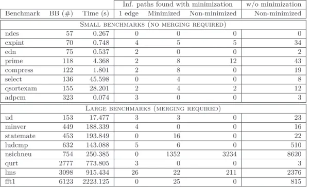
Table 1Results on the Mälardalen benchmarks.

Inf. paths found with minimization w/o minimization Benchmark BB (#) Time (s) 1 edge Minimized Non-minimized Non-minimized

Small benchmarks (no merging required)

ndes 57 0.267 0 0 0 0 expint 70 0.748 4 5 5 34 edn 75 0.537 2 0 0 2 prime 118 4.368 2 8 12 43 compress 122 1.801 2 8 0 19 select 136 45.598 0 4 0 8 qsortexam 155 28.201 2 4 2 12 adpcm 323 0.074 3 0 0 3

Large benchmarks (merging required)

ud 153 17.477 3 3 0 23 minver 449 188.339 4 0 0 16 statemate 453 193.849 0 16 0 22 ludcmp 632 143.088 5 6 0 510 nsichneu 754 250.385 0 1352 3234 8620 qurt 2777 773.805 3 0 0 3 lms 3098 915.434 26 22 211 2376 fft1 6123 2223.125 0 25 0 815

5

Experimental Results

We have run our analysis program on the Mälardalen benchmarks, compiled into ARM binaries by gcc -O1 (minimal optimizations) with non-constant global memory to ensure multiple paths, performed on a 2.90GHz i7-4600M CPU, 4GB memory. Measuring the efficiency of such an analysis is tough for multiple reasons: (a) we do not know how many actual infeasible paths the program contains, (b) since our analysis is targetted to exhibit infeasible paths, but not to exploit them, any measured improvement on the computed WCET estimation is also due to the efficiency of the tool that will exploit these infeasible paths, (c) our infeasible paths are actually sets of infeasible paths, and we do not know how many paths they include. Even if we stop trying to find minimal sets of edges, the analysis cuts paths once they are identified as infeasible, and we do not know how many paths have been cut this way.

Table 1 showcases both the performance of the analysis on this set of benchmark and the powerfulness of the minimization algorithm. The benchmarks are sorted by number of basic blocks (after virtual inlining of function calls). The 17 smallest benchmarks with a size ranging from 2 to 50 basic blocks have been removed, 10 of which gave no results.

The first three result columns show the amount of unique infeasible paths found by the analysis split in three kinds: paths made of only one edge, successfully minimized paths, and paths for which the minimization failed. The last column gives the amount of infeasible paths found when path minimization is disabled. For example, running on “prime” with minimization, the analysis finds 2 + 8 + 12 = 22 infeasible paths, including 10 successfully minimized ones. These 10 short-length paths translate into 43 − 12 = 31 lengthy infeasible paths when no minimization work is done. “fft1” is an extreme: 815 paths have been minimized into 25 paths of an average length of 2.84 edges. We have observed that most of the computing time is spent on SMT solving.

The results look very promising for the bigger benchmarks and the occasional merges of

predicates seem enough to tone down the combinatory explosion without hurting results too much, yet the actual impact on the precision of the computed WCET remains unknown.

6

Conclusion and Future Works

This article proposes a new approach to discover infeasible paths in a binary program. Our solution is a static analysis of (a) a CFG whose blocks are made of machine instructions (abstracted by semantic instructions) and (b) of program data states represented by predic-ates on registers and memories. Unsatisfiability by SMT of predicpredic-ates allows identifying infeasible paths. The result is a list of edges of the program CFG that are forbidden on a feasible execution path. This information is typically used to tighten the precision of the WCET computation.

Although the proposed approach gives promising results, we feel that some infeasible paths remain undiscovered because of (a) too coarse states join operator and (b) of time calculation explosion. Issue (a) is the most important although it means that we have to find smart fixpoints for our predicates. Polyhedra could be an efficient and well-known alternative but we would be bound to linear predicates.

The second issue may be solved by reducing the amount of produced predicates. For example, code slicing would be a good technique to keep only code involved in conditions and therefore to produce only predicates involved in conditions. As a significant part of analysis time is spent in SMT solving, another solution might be to reduce the number of calls to the solver. We have to find a tradeoff during fixpoint computations between the frequency of SMT calls and the minimization of found paths: an SMT call finds infeasible paths but also allows reducing the number of states.

Finally, the infeasible paths found by our approach only concern mutual exclusivity between CFG edges. Our feeling is that quantitative relations, induced by the program semantics, exist between CFG edges and we wish to investigate this domain deeper afterwards.

References

1 C. Barrett, C. Conway, M. Deters, L. Hadarean, D. Jovanovic, T. King, A. Reynolds, and C. Tinelli. CVC4. In 23rd International Conference on Computer Aided Verification

(CAV’11), volume 6806 of Lecture Notes in Computer Science. Springer, 2011.

2 C. Barrett, M. Deters, L. de Moura, A. Oliveras, and A. Stump. 6 Years of SMT-COMP.

Journal of Automated Reasoning, 50(3):243–277, 2013.

3 H. Cassé, F. Birée, and P. Sainrat. Multi-architecture value analysis for machine code. In

WCET’13, pages 42–52. OASICs, Dagstuhl Publishing, 2013.

4 J. Gustafsson, A. Betts, A. Ermedahl, and B. Lisper. The Mälardalen WCET Benchmarks: Past, Present And Future. WCET, 15:136–146, 2010.

5 J. Henry, M. Asavoae, D. Monniaux, and C. Maïza. How to compute worst-case execution time by optimization modulo theory and a clever encoding of program semantics. SIGPLAN

Not., 49(5):43–52, June 2014.

6 V. Suhendra, T. Mitra, A. Roychoudhury, and Ting C. Efficient detection and exploitation of infeasible paths for software timing analysis. In Design Automation Conference, 2006

43rd ACM/IEEE, pages 358–363, 2006.

7 N. Williams, B. Marre, P. Mouy, and M. Roger. PathCrawler: Automatic generation of path tests by combining static and dynamic analysis. In Dependable Computing – EDCC