Thermodynamic aspects of the capture of acid gas from natural gas

HAL Id: tel-01865166

https://pastel.archives-ouvertes.fr/tel-01865166

HAL is a multi-disciplinary open access

archive for the deposit and dissemination of sci-entific research documents, whether they are pub-lished or not. The documents may come from teaching and research institutions in France or abroad, or from public or private research centers.

L’archive ouverte pluridisciplinaire HAL, est destinée au dépôt et à la diffusion de documents scientifiques de niveau recherche, publiés ou non, émanant des établissements d’enseignement et de recherche français ou étrangers, des laboratoires publics ou privés.

Thermodynamic aspects of the capture of acid gas from

natural gas

Tianyuan Wang

To cite this version:

Tianyuan Wang. Thermodynamic aspects of the capture of acid gas from natural gas. Chemical en-gineering. Université Paris sciences et lettres, 2017. English. �NNT : 2017PSLEM061�. �tel-01865166�

iii

To Qiao,

And our parents

v

ACKNOWLEDGMENTS

I would first like to thank my two thesis supervisors, Christophe Coquelet and Elise El Ahmar for their generosity in CTP, for our many exchanges and for their support during these three years of thesis.

I would like to thank Pr. Guy Weireld, Dr.Robin Westacott, Pr. Georgios, Kontogeorgis, Dr. Renaud Cadours for accepting to review my thesis and for their advices. I would also like to thank Pr. Georgios, Kontogeorgis not only for accepting to be the chairman of the thesis committee but also for our discussions during the meetings we had in DTU when I spent unforgettable three months in Denmark thanks to a great team in CERE.

I express in these lines all my thanks for the members of the CTP: Jocelyne and Marie-Claude for helping me on administrative things; Alain, Pascal, Eric, David and Hervé for helping me on the experimental. PhDs, Marco, Fan, Jamal, Martha, and Mauro for our discussions.

Thanks to my colleagues and friends, I enjoyed my stay in Fontainebleau.

vii

INTRODUCTION ... 2

1 ACID GAS REMOVAL FROM NATURAL GAS ... 6

1.1 THE GROWTH OF ENERGY DEMAND OF NATURAL GAS ... 7

1.2 NATURAL GAS RESERVES ... 8

1.3 NATURAL GAS PROCESSING ... 10

1.4 ACID GAS REMOVAL TECHNOLOGIES ... 12

1.4.1 Adsorption ... 12

1.4.2 Membrane ... 12

1.4.3 Low temperature separation ... 13

1.4.4 Physical absorption ... 13

1.4.5 Chemical absorption ... 14

1.5 CHEMICAL ABSORPTION PROCESS ... 14

1.5.1 1 The principal of chemical absorption process ... 14

1.5.2 The types of amines ... 15

1.5.3 Modelling of amine absorption columns ... 18

1.5.3.1 Equilibrium model ... 18

1.5.3.2 Non-equilibrium model (rate-based model) ... 21

1.6 THE IMPORTANCE OF THE THERMODYNAMIC MODEL ... 23

1.7 SCOPE OF THIS THESIS ... 24

2 `EXPERIMENTAL WORK ... 27

INTRODUCTION ... 27

2.1 STATIC-ANALYTIC METHOD: ... 28

2.1.1 Experimental setup ... 28

2.1.1.1 The equilibrium cell ... 29

2.1.1.2 The ROLSITM _{sampler ... 29}

2.1.1.3 Solvent preparation ... 30 2.1.1.4 Gas chromatography ... 32 2.1.1.5 Calibration of detectors ... 34 2.1.2 Results ... 36 2.2 THE GAS STRIPPING METHOD ... 40 2.2.1 Experimental set up ... 40 2.2.2 Chemicals ... 41

2.2.3 Henry’s Law Constant Calculation ... 42

2.2.4 Results for different sulphur component in 14.6 wt% MEA ... 43

2.2.5 Results for CS2 in different solvents ... 46

3 THERMODYNAMIC MODEL ... 49

INTRODUCTION ... 49

3.1 PHASE EQUILIBRIUM CALCULATION ... 51

3.1.1 Vapour Liquid Equilibrium ... 53

3.1.1.1 Dissymmetric approach ... 53

3.1.1.2 Symmetric approach ... 54

3.1.1.3 The mixing rules ... 56

3.1.2 Vapour Liquid Liquid Equilibrium ... 57

3.2 THERMODYNAMIC MODELS FOR ACID GAS REMOVAL ... 58

3.2.1 The Deshmukh–Mather model ... 58

3.2.1.1 Chemical reactions with MDEA ... 59

3.2.1.2 Activity coefficients calculation ... 61

viii

3.2.2 The Cubic Plus Association EoS ... 64

3.2.2.1 Pure component ... 66

3.2.2.2 Mixtures ... 69

3.2.2.3 The new approach to treat Chemical reactions ... 71

4 MODELLING OF NON-REACTIVE SYSTEMS ... 75

INTRODUCTION ... 75

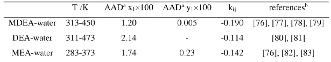
4.1 ALKANOLAMINE-WATER BINARY SYSTEMS ... 77

4.2 ALKANE-WATER-ALKANOLAMINE TERNARY SYSTEMS ... 79

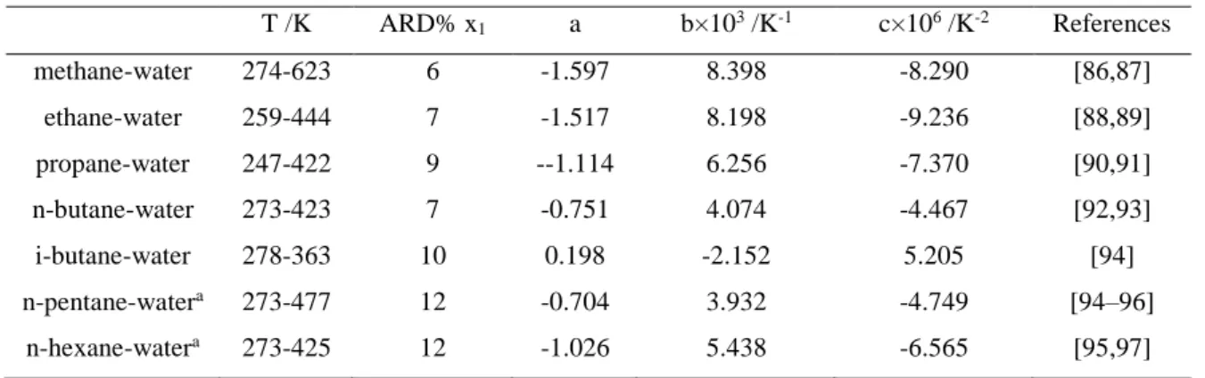
4.2.1 Alkane-water binary systems ... 79

4.2.2 Alkane solubility in aqueous alkanolamine solution ... 80

4.2.3 Temperature of minimum solubility of methane ... 84

4.2.4 Vapour phase prediction ... 87

4.2.5 Alkane solubility prediction at VLLE conditions ... 89

4.2.6 Multi-component alkanes solubilities prediction in aqueous amine solutions ... 92

4.3 AROMATIC-WATER-ALKANOLAMINE TERNARY SYSTEMS ... 94

4.3.1 Aromatics-water binary systems ... 94

4.3.2 Aromatic solubility in aqueous alkanolamine solution ... 97

4.4 MERCAPTAN-WATER-ALKANOLAMINE-METHANE QUATERNARY SYSTEMS ... 100

4.4.1 Mercaptan-methane binary systems ... 100

4.4.2 Mercaptan-water binary systems ... 102

4.4.3 Mercaptan solubility in aqueous alkanolamine solution with pressure adjusted by methane ... 103

4.4.4 Model validation: comparison with our new experimental results ... 106

CONCLUSION ... 108

5 MODELLING OF REACTIVE SYSTEMS ... 110

INTRODUCTION ... 110

5.1 MODELING OF CO2-MDEA-WATER TERNARY SYSTEM ... 111

5.1.1 CO2-water Binary system ... 111

5.1.2 The choice of model parameters for CO2-MDEA-water ternary system ... 113

5.1.2.1 The association scheme of MDEA ... 114

5.1.2.2 kij between CO2-MDEA ... 116

5.1.2.3 The solvation effect between CO2-water ... 118

5.1.3 Model prediction ... 120

5.1.3.1 CO2 solubility ... 120

5.1.3.2 Liquid phase speciation ... 121

5.1.3.3 Enthalpy of absorption... 122

5.1.4 Comparison with Deshmukh–Mather model ... 123

5.2 MODELING OF H2S-MDEA-WATER TERNARY SYSTEM ... 126

5.2.1 H2S-water Binary system ... 126

5.2.2 H2S solubility in aqueous MDEA ... 127

5.2.3 Model prediction ... 129

5.3 MODELING OF CO2-MEA-WATER TERNARY SYSTEM ... 130

5.3.1 Model prediction ... 132

5.3.1.1 Liquid phase speciation ... 132

5.3.1.2 Vapour phase concentration ... 133

5.3.1.3 Enthalpy of absorption... 134

5.4 MODELLING OF H2S-MEA-WATER TERNARY SYSTEM... 136

5.5 MULTICOMPONENT SYSTEM PREDICTION ... 138

5.5.1 CH4-CO2-H2S-H2O quaternary system ... 138

5.5.2 CO2-H2S-H2O-alkanolamine quaternary system ... 138

5.5.3 CO2-H2O-MDEA-CH4 quaternary system ... 141

5.5.4 EM-CO2-MDEA-water-CH4 multi-component system ... 142

ix

CONCLUSION AND FUTURE WORK ... 147 APPENDIX I CALIBRATIONS ... 149 APPENDIX II UNCERTAINTY CALCULATION... 155 APPENDIX III CHROMATOGRAPH OF COS, CS2 AND CO2 IN AQUEOUS 50 WT% MDEA

SOLUTION ... 157 APPENDIX IV LIST OF PUBLICATION ... 158 REFERENCE ... 159

x

List of Symbols

Abbreviations

AAD Average absolute deviation

ARD Average absolute relative deviation

BIP Binary interaction parameter

CPA Cubic Plus Association

CR Combining Rule

DEA Diethanolamine

DMS Dimethyl sulfide

DM Deshmuch Mather model

EM Ethyl mercaptan

E-NRTL Electrolyte Non random two liquids model

EoS Equation of State

FID Flame ionization detector

Func Objective function

HETP Height Equivalent to a Theoretical Plate

GC Gas Chromatography

MEA Monoethanolamine

MDEA Methyl diethanolamine

MM methyl mercaptan

xi

n-BM n-Butyl mercaptan

NRTL Non random two liquids

PR Peng Robinson

ppm Part per million

ROLSI Rapid online sampler injector

SRK Soave – Riedlich - Kwong

SAFT Statistical Associating Fluid Theory

TCD Thermal conductivity detector

UNIFAC Universal quasi chemical

UNIQUAC Universal quasi chemical model Functional activity coefficient model

VLE Vapour – liquid equilibrium

VLLE Vapour – liquid – liquid equilibrium

vdW van der Waals

Latin letter

a energy parameter

ao parameter in energy term

ai activity of component i

A Debye and Hückel parameter

B Debye and Hückel parameter

b co-volume parameter

c Parameter of the equation of state

d Temperature dependent segment diameter

xii

L

f Fugacity in solution

G Gibbs energy

E

g Excess Gibbs energy

g(d) radial distribution function

h Enthalpy

H Henry’s law constant

I Ionic strength based on ionic strength

K Equilibrium constant

 Density

kij Binary interaction parameter in mixing rule

lij Dimensionless constant for binary interaction parameter for the asymmetric

term

mi Molality of species i

M molar mass

N Number of moles

NA Avogadro’s number, [1/mol]

Nc Number of components

Pv _{Vapour pressure}

P Pressure

R Universal gas constant

S Entropy

T Temperature [K]

xiii

vl _{Saturated liquid volume}

x Liquid mole fraction

XAi Mole fraction of component not bonded at site A of component i

y Vapour mole fraction

z initial composition

Zi number of charge of specie i

z Coordination number in the UNIQUAC model of Abrams and Prausnitz (1975)

Greek letters:

 Fugacity coefficient

 Fugacity coefficient in solution

 Activity coefficient

i

 _{Infinite dilution activity coefficient of component i}

 Chemical potential of component i

βij Model binary interaction parameter in DM model

ᵚ Acentric factor

AiBj _{Association volume between site A of component i and site B of component j}

AB _{Strength of interaction between sites A and B.}

 Numerical constant in the EoS

0

 Vacuum permittivity

r

 Relative permittivity (dielectric constant dimensionless)

AiBj

 Association energy between site A of component i and site B of component j

14 Superscript

E Excess property

R Residual property

Sat saturated value

cal Calculated property

exp Experimental property

i,j Molecular species

c Critical property

Ref reference property

L Liquid state V Vapor state * Property at saturation Assoc Association Res residual Subscripts

cal Calculated property

exp Experimental property

i, j Molecular species

0 Reference property

Cal Calculated value

Exp. Experimental value

15

List of table

Table 1-1 : Example of natural gas composition [9] ... 8

Table 2-1. Purity and producer of the used substances ... 31

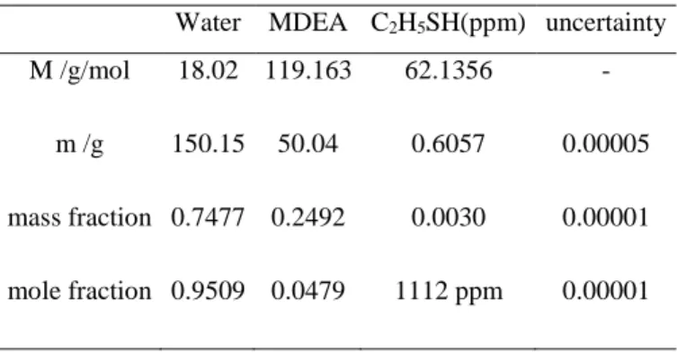
Table 2-2 Composition of prepared 25 wt % MDEA aqueous solution with EM (2281ppm) ... 31

Table 2-3 Composition of prepared 25 wt % MDEA aqueous solution with EM (1112ppm) ... 31

Table 2-4 Composition of prepared 25 wt % MDEA aqueous solution with MM (2438ppm) ... 32

Table 2-5 Parameter setting for GC liquid and vapour analysis. ... 34

Table 2-6 Components and accuracy (typical accuracy values) ... 35

Table 2-7a. Vapour Liquid equilibrium data of MM in aqueous MDEA solution (25 wt% MDEA) (global concentration of MM: 2438 ppm). x corresponds to the standard deviation due to repeatability measurements. u(x) corresponds to the uncertainty u(T)=0.02 K, u(P)=0.0001 MPa ... 37

Table 2-8 CAS Numbers, Purities and Suppliers of Materials. ... 41

Table 2-9 Composition of prepared 14.6 wt % MEA aqueous solution ... 42

Table 2-10 solutes vapour pressures parameters [38] ... 43

Table 2-11 Henry’s Law Constant and infinity dilution coefficient for all the studied mercaptans in MEA aqueous solution, u(H)/H=15%, u(γ∞)/ γ∞=15% ... 45

Table 2-12 Henry’s Law Constant for CS2 in pure water, u(H)=15%, u(γ∞)=15% ... 46

Table 3-1 Equilibrium constants for MDEA-CO2-water ternary system [56] ... 60

The second term of Equation (3.56) represents the short distance interactions between the different molecular or ionic species. This term is empirical. The interaction parameters βij exclude the pairs (i, j) of the same sign. The βij are obtained with a regression of experimental data. According to Dicko et al.[56], only limited pairs of βij are needed to be fitted from experimental data, they are shown in Table 3-2.The adjusted values are presented in the Chapter 5. ... 63

16 Table 3-4 Parameters for calculating Henry’s law constant of solute and saturation pressure of solvent [56] ... 64 Table 3-5 Pure component parameters for non self associating components [65] ... 67 Table 3-6. PR CPA parameters for compounds for association compounds considered in this work [65] ... 69 Table 4-1. Average Absolute Deviation (AAD) for liquid and vapour composition between PR-CPA EoS adjusted data and experimental ones of water with MEA, DEA or MDEA binary system and kij values. ... 77

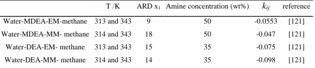
Table 4-2 List of BIPs required representing alkane-water-alkanolamine ternary systems. ... 79 Table 4-3 Comparison between alkane solubility data water with the calculated ones obtained with PR –CPA EoS and a,b and c parameters values... 80 Table 4-4 Comparison between experimental data of alkane solubility in aqueous alkanolamine solutions and the adjusted ones obtained with PR-CPA EoS ... 82 Table 4-5. Methane minimum solubility temperature in aqueous MDEA solution and in pure water predicted by PR-CPA EoS. ... 85 Table 4-6 Hydrocarbon mixture composition from Mokraoui et al. [98] ... 92 Table 4-7 PR- CPA EoS prediction of hydrocarbon mixture solubility in aqueous alkanolamine solutions ... 93 Table 4-8 List of BIPs required representing alkane-water-alkanolamine ternary systems. ... 94 Table 4-9 comparison between experimental data on aromatic solubility in water and adjusted data with PR-CPA EoS, β and a,b,c parameters values ... 95 Table 4-10 comparison experimental data of aromatic solubility in aqueous alkanolamine solutions with PR-CPA EoS ... 99 Table 4-11 List of BIPs required representing mercaptan-water-alkanolamine-methane quaternary systems... 100 Table 4-12: BIPs values and ARD of liquid (x) composition between PR-CPA EoS adjusted data and experimental ones obtained for methane (1) with MM or EM binary system. 100 Table 4-13 : BIPs values and ARD of liquid (x) composition between PR-CPA EoS adjusted data and experimental ones obtained for water (1) with MM or EM binary system. ... 102

17 Table 4-14 kij values and ARD of liquid (x) composition between PR-CPA EoS adjusted

data and experimental ones obtained for MM or EM with water-alkanolamine systems.

... 103

Table 5-1 BIP values and ARD of liquid (x) compositions between PR-CPA EoS adjustment and experimental data for CO2-water binary system. ... 112

Table 5-2 PR-CPA binary parameters for CO2-MDEA-water ternary system ... 113

Table 5-3 Comparison of symmetric and asymmetric approach for CO2-MDEA binary system with PR-CPA EoS. ... 114

Table 5-4 Influence of kij on the asymmetric approach ... 116

Table 5-5 Influence of kij on the asymmetric approach ... 118

Table 5-6 Adjusted parameters for CO2-MDEA-water ternary system ... 123

Table 5-7 kij value and ARD of liquid (x) compositions between PR-CPA EoS adjusted data and experimental ones obtained for H2S –water binary system. ... 126

Table 5-8 Adjusted Binary Interaction Parameters of PR-CPA for H2S-MDEA-water ternary system ... 127

Table 5-9 PR-CPA binary parameters for CO2-MDEA-water ternary system ... 131

Table 5-10 PR-CPA EoS binary parameters for CO2-MDEA-water ternary system ... 136

Table 5-11 Initial composition of CH4-CO2-H2S-H2O mixtures ... 138

Table 5-12 ARD of PR-CPA EoS prediction for CH4-CO2-H2S-H2O quaternary system [140] ... 138

Table 5-13 Experimental data [143] and model prediction data for CO2-MDEA-water-CH4 quaternary system at 10 MPa with 30 wt % MDEA ... 142

Table 5-14 Experimental data from Boonaert et al. [144] and mode prediction by PR-CPA for EM-CO2-MDEA-water-CH4 system at 7 MPa with 25 wt % MDEA... 144

18

List of figures

Figure 1-1 Shares of primary energy source from BP[7] ... 7

Figure 1-2 Global distribution of CO2 content in natural gas reserve [10] ... 9

Figure 1-3. Flow diagram of a typical natural gas processing plant [12] ... 11

Figure 1-4 Typical Amine Flow Diagram[24] ... 15

Figure 1-5 Structural formulae for alkanolamines used in gas treating units ... 16

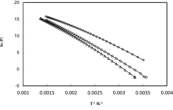
Figure 1-6.Vapour pressures of different alkanolamines as a function of inverse of temperature, data from NIST (◇)=MEA, (○)=DEA, (Δ)=MDEA ... 17

Figure 1-7 Decomposition of the distillation into theoretical stages [32] ... 19

Figure 1-8 Flow patterns on a column tray [32] ... 20

Figure 1-9 1D schematic diagram of a non-equilibrium stage [32] ... 21

Figure 1-10 Illustration of the gas and liquid mass transfer occurring in a segment of packed column during the absorption process [34] ... 22

Figure 1-11 physical property needs of equilibrium (right) and non-equilibrium (left) models [32] ... 23

Figure 2-1. Schematic diagram of apparatus: d. a. u. : Data Acquisition Unit ; DDD : Digital Displacement Display ; DM : Degassed Mixture ; DT : Displacement Transducer ; EC : Equilibrium Cell ; GC : Gas Chromatograph ; LB: Liquid Bath; LS : Liquid Sampler ; LVi : Loading Valve ; MR; Magnetic Rod; P: Propeller; PP : Platinum Probe ; PTh: Pressure transducer for high pressure values; PTl: Pressure transducer for low pressure values; SD : Stirring Device ; SM: Sample Monitoring; CI: Cylindrical tube Injector; TR: Thermal Regulator; Vi: Valve; VP: Vacuum Pump; VS: Vapour Sampler; VVCM: Variable Volume Cell for Mixture. ... 28

Figure 2-2 Cross sectional view of Electromagnetic ROLSI® ... 30

Figure 2-3 Gas chromatograph for liquid and vapor phase analysis (simplified analytical circuit), A1 A2 : Column; AG: auxiliary gas; C: commuting valve; FID: Flame Ionization Detector; I: Injectors; O: Oven; T: Thermal conductivity detector; VS: Vapor phase sampler; LS: Liquid phase sampler.[37] ... 33

19 Figure 2-4. Oven temperature programming as a function of time (min) from 333 to 518 K.

... 34

Figure 2-5. GC gas/liquid injector [35] ... 35

Figure 2-6 Flow diagram of the equipment: BF, bubble flow meter; C, chromatograph; D, dilutor; d.a.s., data acquisition system; He,helium cylinder; E1, E2, heat exchangers; FE, flow meter electronic; FR, flow regulator; L, sampling loop; LB, liquid bath; O, O-ring; PP,platinum resistance thermometer probe; S, saturator; SI, solute injector; Sp, septum; SV, sampling valve; TR, temperature regulator;VSS, variable speed stirrer ... 40

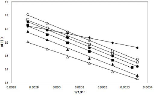
Figure 2-7 Logarithm of Henry’s Law Constant of different component in14.6% MEA weight fractions as a function of the inverse of temperature (Δ: MM, ▲: EM,  DMS, : nPM; : iPM, ●: nBM, ○: iBM). ... 46

Figure 2-8View of the dilutor cell after introducing CS2 ... 47

Figure 3-1 Distribution of anions and cations in the ionic atmosphere [59] ... 62

Figure 3-2 Association schemes for associating components [66] ... 68

Figure 3-3 Solvation between water carbon dioxide [70] ... 70

Figure 3-4 association schemes developed in this research ... 72

Figure 3-5 Reaction mechanism between CO2 and MEA (asymmetric model) ... 73

Figure 4-1. Comparison between experimental data (symbols) and adjusted ones using PR-CPA EoS (solid lines) for MEA-water binary system; (×) =333 K:Lenard et al. [32], (□)=343 K:Kim et al. [26], (△)=353 K :[26], (○)= 363 K:Tochigi et al. [33], (◇)=373 K [26]. ... 78

Figure 4-2. Comparison between experimental data (Kim et al. [26], symbols) and adjusted ones using PR-CPA EoS (solid lines) for MDEA-water binary system; (×)=313 K, (△)=333 K, (○)= 353 K, (◇)=373 K. ... 79

Figure 4-3. (b. is the zoom of a.) Comparison between experimental data from Jou et al. [21] for propane solubility in 35 wt % aqueous MDEA solution and adjusted data using PR-CPA EoS (solid lines). (×) =273 K, (□)=298 K, (△)=313 K (○)=323 K, (*)=348 K, (■)=398 K, (▲)=398 K, (●)=423 K, dashed line: VLLE interface. ... 83

Figure 4-4 Propane solubility in function of DEA concentration (up to 65 wt %) at 313K, 1.724 MPa, symbol :experimental data from Jou et al.[54], solid line: calculated data using PR-CPA EoS ... 84

20 Figure 4-5 PR-CPA EoS prediction on the ratio of methane solubility and the minimum solubility at 75 bar. dotted line=25 wt % MDEA, dashed line=35 wt % MDEA, solid line=50 wt % MDEA ... 85 Figure 4-6 PR-CPA EoS prediction of the temperature of minimum solubility of methane as function of MDEA concentration at different pressure, symbols: PR-CPA EoS prediction, (×) =5 MPa, (□)=7.5 MPa, (○)=10 MPa, lines :linear correlation ... 86 Figure 4-7. PR-CPA EoS prediction of the temperature of minimum solubility of methane as function of pressure in different aqueous MDEA solutions symbols: PR-CPA EoS

prediction (□) =50 wt % MDEA, (×)=35 wt % MDEA, (○)=25 wt % MDEA and (△)=pure

water, lines: linear correlation ... 87 Figure 4-8 Comparison between experimental data from Caroll et al. [106] for water content in propane rich phase of propane-MDEA(35 wt %)-water ternary system and predicted data using PR-CPA EoS (solid lines). (◆) =273K, (■)=298K, (▲)=323K, (×)=348K, (*)=373K, (●)=398K, (+)=423K ... 88 Figure 4-9. Comparison between experimental data from Mokraoui et al. [17] for solubility of ethane in aqueous MDEA solution and predicted data using PR-CPA EoS (solid lines). (△) =Pure water, (×)=25 wt % MDEA, (□)=50 wt % MDEA. ... 90 Figure 4-10. Comparison between experimental data from Mokraoui et al. [17] for solubility of propane in aqueous MDEA solution and predicted data using PR-CPA EoS (solid lines). (△) =Pure water, (×)=25 wt % MDEA, (□)=50 wt % MDEA. ... 91 Figure 4-11. Comparison between experimental data from Mokraoui et al. [17], Jou et al. [44] for solubility of nbutane in aqueous MDEA solution and predicted data using

PR-CPA EoS (solid lines). (△) =Pure water [17], (×) =25 wt % MDEA [17], (○)=35 wt %

MDEA [44], (□)=50 wt % MDEA [17],. ... 92 Figure 4-12 Comparison between experimental data (symbols) and adjusted ones using PR-CPA EoS (solid lines) for benzene solubility in water; (□): Jou et al. [112], (△) : Valtz

et al... 96 Figure 4-13 Comparison between experimental data (symbol) and adjusted ones using PR-CPA EoS (solid lines) for water solubility in benzene rich phase; (□): Jou et al. [112] . 97

21 Figure 4-14 Solubility of benzene in aqueous MDEA solution at VLLE condition. Experimental data: Valtz et al.[116]. (△) Pure water; (×) 25 wt % MDEA; (□) 50 wt %

MDEA. Solid lines: PR-CPA model prediction ... 98 Figure 4-15 Phase diagram (P-x-y) of methane-EM binary system at 272K, symbol: experimental data [117], Lines: adjusted data obtained with PR-CPA EoS. ... 101 Figure 4-16 Phase diagram (P,x,y)of methane-MM binary system at 304K, symbol: experimental data [117], Lines: adjusted data obtained with PR-CPA EoS. ... 101 Figure 4-17 Phase diagram (P,x,y)of water-MM binary system at 470K, symbol: experimental data from Awan et al. [117], Lines: adjusted data obtained with PR-CPA EoS. ... 102 Figure 4-18 Comparison between experimental data from Jou et al. [120] and ones obtained with PR-CPA EoS for EM-water –MDEA system (50 wt% MDEA): a. EM solubility, b. Methane solubility and c. EM composition in vapour phase. ... 104 Figure 4-19 Comparison between experimental data from Jou et al. [120] and ones obtained with PR-CPA EoS for MM-water –MDEA system (50 wt% MDEA): a. MM solubility, b. Methane solubility and c. MM composition in vapour phase. ... 105 Figure 4-20 Henry’s law constant in function of pressure for EM in aqueous MDEA solution. Symbols: experimental data this work (×) = 2000 ppm EM, (●) = 1000 ppm EM, Solid lines: model prediction for systems with 1000 ppm EM, dotted lines model prediction for systems with 2000 ppm EM. ... 107 Figure 4-21 Henry’s law constant in function of pressure for MM in aqueous MDEA solution. Symbols: experimental data obtained with 1 000 ppm of MM as initial composition in this work (×) = 333 K , (□) = 365 K . Dotted lines model prediction .. 107 Figure 4-22 Deviations of hydrocarbon and mercaptan solubility in aqueous alkanolamine solution. C1=methane, C2=ethane, C3=propane, C4=butane, C5=pentane, C6=hexane, B=benzene, T=toluene, MM=methyl mercaptan, EM=ethyl mercaptan ... 108 Figure 5-1 Comparison of experimental CO2 solubility in water and adjusted values by

PR-CPA EoS, solid line: without solvation, dotted lines: with solvation. symbol: experimental data from Valtz et al. [122] ; (○)=298 K , (□)=308 K (*)=318 K, ... 112 Figure 5-2 Comparison of total pressure of CO2-MDEA-water ternary system with 32 wt%

22 approach, Dotted Lines: with symmetric approach. Symbols: experimental data from Kuranov et al. [125]. (◆)=313 K, (▲)=333 K, (■)=373 K,( ●)=393 K，(×)=413 K . 115 Figure 5-3 Comparison of total pressure of CO2-MDEA-water ternary system with 32 wt%

MDEA and adjusted values obtained with PR-CPA EoS. Solid lines: with kij=0, Dotted

Lines: with adjusted kij. Symbols: experimental data from Kuranov et al. [125]. (◆)=313

K, (▲)=333 K, (■)=373 K, (●)=393 K，(×)=413 K ... 117 Figure 5-4 Comparison of total pressure of CO2-MDEA-water ternary system with 32 wt%

MDEA and adjusted values obtained with PR-CPA EoS. Solid lines: with CO2-water

solvation, Dotted Lines: without CO2-water solvation. Symbols: experimental data from

Kuranov et al. [125]. (◆)=313 K, (▲)=333 K, (■)=373 K, (●)=393 K，(×)=413 K . 119 Figure 5-5 Comparison of total pressure of CO2-MDEA-water ternary system with 19 wt%

MDEA and adjusted values obtained with PR-CPA EoS. Solid lines: with CO2-water

solvation, Dotted Lines: without CO2-water solvation. Symbols: experimental data from

Kuranov et al. [125]. (◆)=313 K, (▲)=333 K, (■)=373 K, (●)=393 K，(×)=413 K . 120 Figure 5-6 Prediction of total pressure of CO2-MDEA-water ternary system with 25 wt%

MDEA with PR-CPA EoS. Solid lines: with CO2-water solvation, Dotted Lines: without

CO2-water solvation. Symbols: experimental data from Sidi-Boumedine et al. [126].

(◆)=298 K, (▲)=313 K, (■)=348 K ... 120 Figure 5-7 Prediction of liquid phase electrolytes speciation of CO2-MDEA-water ternary

system with 30 wt % MDEA at 313K. Solid line: MDEA, dotted line: HCO3-1 symbol:

experimental data from Jakobsen et al. [127]: (△)=HCO3-1, (○)=MDEA ... 121

Figure 5-8 Prediction of enthalpy of absorption of CO2-MDEA-water ternary system with

20 wt % MDEA. Lines: PR-CPA EoS prediction, symbols: experimental data from Gupta et al. [129] ... 122 Figure 5-9 Comparison of total pressure of CO2-MDEA-water ternary system with 32 wt%

MDEA and adjusted values obtained with PR-CPA .Solid lines: PR-CPA EoS, Dotted Lines: DM model. Symbols: experimental data from Kuranov et al. [125]. (◆)=313 K, (▲)=333 K, (■)=373 K, (●)=393 K，(×)=413 K ... 124 Figure 5-10 Comparison of total pressure of CO2-MDEA-water ternary system with 19 wt% MDEA and adjusted values obtained with PR-CPA EoS .Solid lines: PR-CPA, Dotted Lines:

23 DM model. Symbols: experimental data Kuranov et al. [125]. (◆)=313 K, (▲)=333 K, (■)=373 K, (●)=393 K，(×)=413 K ... 125 Figure 5-11 Prediction of total pressure of CO2-MDEA-water ternary system with 25 wt%

MDEA. solid lines: PR-CPA EoS, Dotted Lines: DM model. Symbols: experimental data from Sidi-Boumedine et al. [126]. (◆)=298 K, (▲)=313 K,( ■)=348 K ... 125 Figure 5-12 Comparison of experimental H2S solubility in water and adjusted values

obtained with PR-CPA, symbol: experimental data from Selleck et al. [132]; (□)=311K (x)=344K, (○)=377 K , solid lines: PR-CPA EoS. ... 126 Figure 5-13 Comparison of total pressure of H2S-MDEA-water ternary system with 48 wt%

MDEA and adjusted values obtained with PR-CPA EoS. Symbols: experimental data from Sidi-Boumedine et al. [126] . Solid lines: PR-CPA EoS adjusted data. (◆)=313K, (■)=373 K. ... 128 Figure 5-14 Comparison of total pressure of H2S-MDEA-water ternary system with 20 wt%

MDEA and adjusted values obtained with PR-CPA EoS. Symbols: experimental data from Bhairi et al. [133] . Solid lines: PR-CPA EoS adjusted data. (◆)=311 K, (▲)=338 K, (■)=388 K. ... 129 Figure 5-15 Prediction of total pressure of H2S-MDEA-water ternary system with 35 wt%

MDEA. Symbols: experimental data from Jou et al. [134] . Solid lines: PR-CPA EoS. (◆)=313 K, (▲)=373 K. ... 130 Figure 5-16 Comparison of total pressure of CO2-MEA-water ternary system with 30 wt%

MEA and adjusted values obtained with PR-CPA. Solid lines: experimental data from Jou et al. [135]. (▲)=298 K, (●)=333 K， (×)=353 K, (+)=393 K ... 131 Figure 5-17 Prediction of liquid phase electrolytes speciation of CO2-MEA-water ternary

system with 30 wt % MEA at 313.15 K. Solid line: HCO3-1, dashed line: MEACOO-, dotted

line: MEA+MEAH+, symbols: experimental data from Hilliard et al. [136] (△)=HCO3

-1_{,(◇)= MEACOO}- _{(○)=MEA+MEAH}+ _{from Hilliard [137], (▲)=HCO}

3-1,(◆)=

MEACOO- (●)=MEA+MEAH+. ... 132

Figure 5-18 Prediction of vapour phase composition of CO2-MEA-water ternary system

with 30 wt % MEA at 333.15 K Lines predicted by PR-CPA EoS, Solid line: ywater, dashed

24 Figure 5-19 Prediction of vapour phase composition of CO2-MEA-water ternary system

with 30 wt % MEA at 313.15 K Lines predicted by PR-CPA EoS, Solid line: ywater, dashed

line:yMEA, symbol: experimental data from Hilliard et al. [137] (▲)=ywater,(◆)= yMEA 134

Figure 5-20 Prediction of enthalpy of absorption of CO2-MEA-water ternary system with

30 wt % MEA at 313.15, Solid line PR-CPA EoS, symbol: experimental data from Hilliard et al. [137] ... 135 Figure 5-21 Prediction of enthalpy of absorption of CO2-MEA-water ternary system with

30 wt % MEA at 393.15, Solid line PR-CPA EoS, symbol: experimental data from Hilliard et al. [137] ... 135 Figure 5-22 Comparison of H2S partial pressure of H2S-MEA-water ternary system with

30 wt% MEA and adjusted values obtained with PR-CPA. Solid lines: experimental data from Lee et al. [139]. (♦)=298 K, (▲)=313 K, (■)=333K, (●)=353 K， (×)=373 K, (+)=393 K ... 137 Figure 5-23 Prediction of H₂S partial pressure in a CO₂-H₂S-water-MEA(15 wt%) quaternary system : experimental data from Lee et al. [139]. P=0.001 for student t-test ... 139 Figure 5-24 Prediction of CO₂ partial pressure in a CO₂-H₂S-water-MEA(15 wt%) quaternary system : experimental data from Lee et al. [139]. P=0.033 for student t-test ... 140 Figure 5-25 Prediction of CO₂ partial pressure in a CO₂-H₂S-water-MDEA(50 wt%) quaternary system : experimental data from Jou et al. [142]. P=0.057 for student t-test ... 140 Figure 5-26 Prediction of H2S partial pressure in a CO₂-H₂S-water-MDEA(50 wt%)

quaternary system : experimental data from Jou et al. [142] P=0.073 for student t-test ... 141 A-0-1 FID calibration and deviation for EM ... 149 A-0-2 FID calibration and deviation for CH4... 150

A-0-3 TCD calibration and deviation for CH4 ... 151

A-0-4 TCD calibration and deviation for MM ... 152 A-0-5 TCD calibration and deviation for water ... 153

25 A-0-6 pressure calibration and deviation ... 154 Figure 0-1 Chromatograph solute peak area (A) as a function of time for CS2 in 50 wt%

MDEA aqueous solution at 328 K. ... 157 Figure 0-2 Chromatograph solute peak area (A) as a function of time for COS and CO2 in

1

2

Introduction

Among fossil fuels, natural gas is the cleanest, in terms of CO2 emission, burn efficiency

and amount of air pollutant [1]. Methane is the prevailing element of natural gas; therefore, there are also a variety of impurities. In fact, it contains usually considerable amounts of acid gases (CO2, H2S) which can lead to corrosion in equipments and pipelines if water is

present. Mercaptans are known as toxic molecules with undesirable odor, and fuel combustion of mercaptan molecules can produce SO2 which is undesirable chemical, they

can cause environmental issues. Acid gases and mercaptans must be removed from natural gas until acceptable standard. The treated natural gas contains as maximum as 2% of CO2,

2–4 ppm of H2S and 5–30 ppm of total mercaptans [2]. Chemical absorption with

alkanolamines [3] (such as monoethanolamine (MEA), diethanolamine (DEA), methyldiethanolamine (MDEA)) is the most well-established method to separate acid gas from natural gas. Acid gases react with alkanolamines in the absorber to form electrolyte species, mercaptans and hydrocarbons do not react with alkanolamines molecules, and they are physically absorbed by aqueous alkanolamine solution. The context and the absorption process will be presented in chapter 1. The main aim of this thesis is to develop an accurate thermodynamic model to describe alkane, aromatic and Mercaptans (methane, ethane, propane, n-butane, n-pentane, n-hexane, benzene, toluene, and Methyl Mercaptan, Ethyl Mercaptan) solubilities in aqueous alkanolamine solution, to describe acid gases (CO2,H2S)

solubilities in aqueous alkanolamine solutions, and to predict other crucial properties like: electrolyte concentration, vapor phase composition (mostly water content), and to predict phase diagram for multi-component system containing CO2-H2

S-alkanolamine-water-hydrocabon-mercaptan.

In addition, some experimental works were carried out. Methyl and Ethyl mercaptan solubility in aqueous MDEA partition coefficient was determined at three pressures up to 7MPa, at two temperatures of 333 and 365 K, by using a static-analytic method [4]. The other part of experimental work concerns the measurement of apparent Henry’s law

3

constants and infinite dilution activity coefficient for different sulphur component (MM, EM, nPM, iPM, nBM, iBM, DMS) in aqueous MEA solution by using gas stripping method [5]. The experimental set-ups and results are shown in chapter 2.

Chapter 3 describes the thermodynamic models involved in this work. Two different approaches have been presented: the symmetric and the dissymmetric approaches. The PR-CPA EoS has been chosen as the symmetric approach. It has an explicit part to account for hydrogen bonding, making it well suited to describe interested systems where water and alkanolamines molecules form hydrogen bonds between them and themselves (self and cross associations). Alkanes are considered as non-associating components. However, due to the presence of –OH or –SH functional group, aromatic and mercaptans are considered as solvated components. Unlike alkanes, aromatics and mercaptans, for CO2 and H2S, the

chemical reaction between CO2 / H2S – alkanolamine are treated as strong cross association

between them, the electrolytes formed after chemical reactions are considered as weak electrolyte which are neglected. The Desmukh–Mather model [6] has been chosen as the dissymmetric approach. This model utilizes the extended Debye–Hückel expression to describe all the activity coefficients of electrolyte species for long distance interactions; it uses an EoS and Henry’s law constant to represent the vapour phase. This model is widely used in acid gas-amine-water systems modelling, it is considered as a bench mark model to be compared with our PR-CPA EoS.

Chapter 4 summarizes the results of non-reactive components solubilities (including methane, ethane, propane, n-butane, n-pentane, n-hexane, benzene, toluene, and ethyl-benzene) and mercaptans (MM and EM) in aqueous MDEA, DEA and MEA solutions in VLE, LLE, and VLLE conditions will be treated with PR-CPA EoS. Different thermodynamic properties such as the temperature of minimum solubility, water content, and solubility of two alkanes mixtures in aqueous alkanolamine solutions will be predicted by PR-CPA for model validation. Moreover, experimental data measured in this work will be compared with PR-CPA EoS predictions.

In chapter 5, different configurations of the PR-CPA EoS with the pseudo chemical reaction approach will be investigated to better represent the solubility of acid gas solubility

4

in aqueous alkanolamine solution. CO2-MDEA-water ternary system is assigned to be the

example system to investigate. The PR-CPA EoS performance will compared to Deshmukh–Mather model results for this system. Different thermodynamic properties such as VLE, liquid phase speciation, enthalpy of absorption, and vapor phase composition will be predicted by PR-CPA EoS for model validation. The PR-CPA EoS will be also used to H2S-MDEA-H2O, CO2-MEA-H2O, and H2S-MEA-H2O ternary systems. And different

multicomponent systems such as CO2-H2S-H2O-CH4, CO2-H2S-MEA-H2O, CO2-H2

S-MDEA-H2O, CO2-MDEA-H2O-CH4 CO2-MDEA-H2O-CH4-EM systems will be predicted

by PR-CPA EoS.

5

Chapter 1 Acid gas removal from natural

gas

6

1 Acid gas removal from natural gas

Introduction

Chapter 1 describes the general context of natural gas treatment. The natural gas processing is introduced from upstream to downstream. Different technologies of gas treatment are briefly presented, such as adsorption, membrane, low temperature separation, physical absorption, and chemical absorption. This thesis focus on the chemical absorption, the principal of this process and different types of solvent are detailed in this chapter. The importance of thermodynamic model is highlighted during the modelling of absorption column. The objectives of this work is listed in the end of this chapter.

Le chapitre 1 décrit le contexte général du traitement du gaz naturel. Le traitement du gaz naturel est introduit de l'amont vers l'aval. Différentes technologies de traitement des gaz sont brièvement présentées, telles que l'adsorption, la membrane, la séparation à basse température, l'absorption physique et l'absorption chimique. Cette thèse se concentre sur l'absorption chimique, le principe de ce processus et les différents types de solvants sont détaillés dans ce chapitre. L'importance du modèle thermodynamique est mise en évidence lors de la modélisation de la colonne d'absorption. Les objectifs de ce travail sont présentés à la fin de ce chapitre.

7

1.1 The growth of energy demand of natural gas

The world’s population will increase by 1.5 billion people to reach 8.8 billion people by 2035. Over the same period, the world’s economy is estimated to be doubled [7]. Consequently, the demand of energy will be strongly increased, new energy sources with lower carbon content are under development. Hence natural gas is a major energy transition to meet growing global needs, it represents 24% of total primary energy in 2014. Natural gas is known as the cleanest of all fossil fuels, because it emits 30% less CO2 than oil and

50% less than coal to generate the same amount of heat [8]. The demand of natural gas is still increasing, the estimation is 1.8% per year [7], see Figure 1-1.

Figure 1-1 Shares of primary energy source from BP[7]

The growth natural gas demand in the world leads to a reassessment of the development potential of natural gas with high acid gas concentration reserves and shale gas reserves that were previously considered economically unsustainable.

8

1.2 Natural gas reserves

Natural gas is formed from the decomposition of plants, animals and micro-organisms. The most widely accepted theory states that fossil fuels are usually formed when organic materials are decayed and compressed under the earth’s crust at high pressure and for a very long time (millions of years). Usually, natural gas consist principally of methane (70%-90% on molar composition) and hydrocarbons (ethane, propane, butane, pentane, hexane, and Benzene, Toluene, Ethyl benzene and Xylenes). However, there may exist various impurities in natural gas reserves, we can cite CO2, H2S, sulphur components and

water. A typical composition of natural gas is shown in Table 1-1.

Table 1-1 : Example of natural gas composition [9]

Components Composition /mole %

Methane 84.07 Ethane 5.86 Propane 2.20 i-Butane 0.35 n-Butane 0.58 i-Pentane 0.27 n-pentane 0.25 n-Hexane 0.28

n-Heptane and heavier 0.76 Carbon dioxide 1.30 Hydrogen sulphide 0.63

Nitrogen 3.45

The composition of natural gas is related to the type, depth and location of the underground reservoirs of porous sedimentary deposit and the geology of the area. 40% of natural gas reserves are acid gases, i.e. the concentration of CO2 and H2S is considerable. Middle

9

Eastern and central Asian countries have the most important fields, and the concentration of acid gas vary from the location of the natural gas reservoir see Figure 1-2.

Figure 1-2 Global distribution of CO2 content in natural gas reserve [10]

Acid gases, majority including CO2, H2S and other sulphur species, need to be removed

down to sufficiently low levels to meet transportation specification. In fact, acid gases can lead to corrosion in equipments and pipelines if water is present. Corrosion is defined as an irreversible deterioration of a material because of a chemical reaction with its environment. If the reaction continues with the same intensity, the metal can be completely converted into metal salts.

Mercaptans and other sulphur components may also exist in natural gas reserves. Mercaptans are known as toxic molecules with undesirable odour, and fuel combustion of mercaptan molecules can produce Sulphur dioxide SO2 which is undesirable chemical. SO2

can cause environmental issues like acid rain.

The treated natural gas must contain as maximum as 2% of CO2, 2–4 ppm of H2S and 5–

10

removal technologies have been developed in the last few decades, such as: absorption, adsorption, membrane and low temperature separation technologies. The choice of technology depends on the partial pressure of acid gases in the fuel gas and expected purity of treated gas. Different technologies can be combined in order to benefit from the advantages of each process. Those technologies will be shortly presented in section 1.4.

1.3 Natural gas processing

A typical flow diagram of natural gas processing is shown in Figure 1-3. It shows how raw natural gas is processed into sales gas pipelined to the end user markets. It also displays the list of products during to the natural gas processing. The products include [11]:

 Sales gas (mainly methane)  Ethane

 Natural-gas condensate  Elemental sulphur

 Natural-Gas Liquids (NGL): propane, butanes and C5+

Raw natural gas is generally collected from a group of gas wells and is treated at the same collection site for water and natural gas condensate removal. The condensate is usually transported to an oil refinery and the water is disposed as waste. Then the raw gas is passed to an acid gas removal plant in order to remove H2S, CO2 and other sulphur components

(mercaptans, COS, CS2. Etc). There are many processes available for this purpose, they are

briefly introduced in next section, but chemical absorption with amine is the most historical and well established process, it is detailed in next section.

11

Figure 1-3. Flow diagram of a typical natural gas processing plant [12]

The acid gases are sent to a sulphur recovery unit which converts the H2S into elemental

sulphur or sulphuric acid. The Claus process is by far the most well-known process for sulphur recovery [13].

After passing though dehydration unit, mercury removal unit and nitrogen rejection unit, treated gas is sent to the NGL recovery unit. In this unit, gas can be divided into two parts: one part in gaseous form which contains a lot of methane and ethane, and second part in liquid form which is mainly composed of propane, butane and heavier hydrocarbons (C5 and above). The sales gas is delivered to the customer by pipeline or tanker as liquefied natural gas (LNG).

12

1.4 Acid gas removal technologies

During the near decades, several technologies such as adsorption, membrane, low temperature separation, physical absorption and chemical absorption have been developed in the aim of acid gas removal from natural gas. Each technology has its advantage and limitation, and is adapted to different situations. The combination of those technologies is also possible. This thesis focus on the chemical absorption process which is the most established one among those technologies.

1.4.1 Adsorption

Pressure Swing Adsorption (PSA) [14] is a gas separation process in which the adsorbent is regenerated by reducing the partial pressure of the adsorbed component. There are three main types of adsorbent: activated carbon, synthetic zeolites and Metal-Organic FrameWorks (MOFs). The main characteristics of an adsorbent are the selectivity, the effective adsorption amount, the mass transfer rate, and the heat of adsorption. The adsorption systems are particularly suited for medium scale processes but not suitable for large scale industrial acid gases capture.

1.4.2 Membrane

Membrane separation processes [15] can separate selectively acid gases from natural gas. They can be applied for high pressure feed gas containing high acid gas concentration. They are based on differences in permeabilities of the gas flowing through the membrane. The permeability of gases is related to the nature of the permanent species (size, shape, and polarity), and the physical-chemical properties of the membrane itself. Nowadays, there are principally two types of membrane which are commercially used for acid gas separation: polymeric membranes and inorganic membranes. Generally, polymeric membranes have good intrinsic transport properties, high processability and low cost[15]. However, inorganic membranes which are more expensive than polymeric membranes are more

13

preferment in terms of selectivity, temperature and wear resistance, chemically inertness [16].

1.4.3 Low temperature separation

Cryogenic separation is also known as low temperature distillation; it uses a very low temperature for purifying gas mixtures in the separation process [17]. Cryogenic separation is commercially used to liquefy and purify CO2 from natural gas only containing high CO2

concentrations (typically greater than 50%). The principle of cryogenic separation is condensation of gases. When the temperature is below the boiling point of CO2, it begins

to condense separate and turns into a liquid state. For other gases in natural gas, each of them will turn to a liquid at a different point, so they can be separated into pure components by using pressure and temperature control. The advantages of this process are the suitability to liquefy and purify the feed gas with high concentration of CO2 and for producing a liquid

CO2 ready for transportation by pipeline and does not require compression. The main

disadvantage of cryogenic separation is that the process is highly energy intensive for regeneration and can significantly decrease the overall plant efficiency when applied to streams with low CO2 concentration.

1.4.4 Physical absorption

Physical absorption processes [18] are the type of absorption processes where the solvent interacts only physically with acid gases. This process can be used when the feed gas is characterized by high CO2/H2S partial pressure and low temperatures. CO2/H2S is released

at atmospheric pressure. The existence of heavy hydrocarbon in the feed gas restricts the wide use of physical solvent. In addition, low acid gases partial pressures may also discourage the application of physical solvents. The choice of physical solvent is case dependent, for example: methanol is a physical solvent process that has been used for removing CO2, Selexol [19] and Glycol [20] are effective for capturing both CO2 and H2S,

Glycerol carbonate [21] has high selectivity for CO2 over H2S. The disadvantage of this

14 1.4.5 Chemical absorption

Chemical absorption processes are used to remove acid gases by aqueous action chemical reaction between a solvent with the gases. These processes use a solvent, either an alkanolamine (amine process [22]) or an alkali-salt(hot potassium carbonate processes [23]) in an aqueous solution. The amine process is widely used to purify natural gas with a wide range of partial pressure on acid gases, and it has lower equipment and operation cost. The common amine based solvents used for the absorption process are MEA, DEA and MDEA that reacts with the acid gas (CO2 and H2S). H2S and CO2 can be dissociated from aqueous

amine solution by heat.

1.5 Chemical absorption process

1.5.1 1 The principal of chemical absorption process

Absorption with chemical solvents based on amine has been widely used for the removal of acid gas from natural gas in the gas processing industry. Alkanolamines are the most commonly used solvent for acid gas removal process. As shown in Figure 1-4, the amine absorption process consists two columns: “absorber” (contactor) and “regenerator” (stripper). In the absorber, amine solution is in counter current with the feed gas stream, and acid-base reaction takes place between acid gases impurities and amine solution. The treated gas stream leaves at the top of the absorber and goes for further process. At the meantime, the amine solution becomes loaded with acid gases, also called “rich amine”. It should be noted that hydrocarbons and aromatics are also physically dissolved in rich amine solution in the absorber. Therefore, the rich amine solution is sent to one or two flush drums in order to recover dissolved hydrocarbons. The recovered hydrocarbons are used as plant energy source. Before going into the top of regenerator, the rich amine solution is heated by lean amine stream in a heat exchanger. When the rich amine solution flows down from the top of the regenerator to the reboiler, the chemical bends between acid gases and amines are broken by the heat. Acid gases are released and exit from the top

15

of the regenerator, they can be sent to sulphur recovery units. The lean amine solution leaves from the bottom of the regenerator and then goes though the filtering and skimming unit for removing heavy liquid hydrocarbons.

Figure 1-4 Typical Amine Flow Diagram[24]

Since the reactions between acid gases and amines are exothermic, the capacity of absorption is more appreciate at lower temperature. However, the reaction rate is very slow at lower temperature. Typically, in amine process, absorber is operated at 40 °C which is a compromise between absorption capacity and reaction rate. The absorber operating pressure is typically 7 MPa. For the regenerator, although the regeneration of amine is better at higher temperature, high temperature could lead to the degradation of amine molecules and corrosion of equipment. Therefore, the typical operating temperature of the regenerator is around 120 °C. The operational pressure of regenerator is around 0.1-0.2 MPa.

1.5.2 The types of amines

Flash drum Inlet separator Contactor Stripper Outlet separator Sour gas Sweet gas Acid gas Condenser Reclaimer Heat Reboiler Cooler

Lean solvent booster Rich/lean

Exchanger

Fig 21-4 Typical Gas Sweetening by Chemical Reaction

Solvent Tank

Flash Drum

16

Nowadays, MonoEthanolAmine (MEA), DiEthanolAmine (DEA), and MethyDiEthanolAmine (MDEA) are the most commonly used to purify natural gas, their structures are shown in Figure 1-5.

Figure 1-5 Structural formulae for alkanolamines used in gas treating units

Alkanolamines contain both the alcohol functional groups -OH and the amine functional groups -NH. Due to alcohol functional groups, alkanolamines are totally miscible with water. Alkanolamine is basic because of the presence of amine functional groups. Here, R represents the functional group HOCH2CH2-, MEA has the chemical formula RNH2, DEA

has R2NH and MDEA has R2N-CH3. The reaction between H2S and the alkanolamines can

generally be represented by (we take MEA as an example):

2 2 [ 3] [ ]

RNH H S RNH  HS  (0.1)

The reactions are instantaneous, and occur with primary, secondary and tertiary amines. However, reactions with CO2 depend on the nature of the alkanolamine molecule. Primary

and secondary amines react with CO2 and form carbamate, it can be written as (we take

MEA as an example):

2 2 2 [ ] 3

RNH CO H O RNH COOH O (0.2)

Ternary alkanolamines (MDEA) cannot directly react with CO2, because there is no proton

on the nitrogen atom. Therefore, CO2 reacts firstly with water to form carbonic acid

(H2CO3), and then carbonic acid reacts with the alkanolamine. It can be written as:

2 3 2 2 [ 2 4] 3

R NCH CO H O R NCH HCO (0.3)

Primary and secondary amines react simultaneously with both H2S and CO2, tertiary

17

be used to selective capture of H2S [25]. The selective removal and other advantages of

MDEA make it the most widely used amine in natural gas treatment industry: lower regeneration energy required compared to MEA and DEA; significantly lower vapour pressure, see Figure 1-6; higher absorption capacity; very low corrosion rate; higher chemical stability, lower capacity for absorption of hydrocarbons [26]. Those advantages of MDEA result in lower energy consumption for solvent regeneration, smaller equipment size and lower plant cost. Moreover, additives such as piperazine can be used to increase the rate of reaction between CO2 and MDEA, make it suitable for simultaneous removal of

H2S and CO2 [27]. However, MDEA is more expensive than MEA and DEA.

Figure 1-6.Vapour pressures of different alkanolamines as a function of inverse of temperature, data from NIST (◇)=MEA, (○)=DEA, (Δ)=MDEA

MEA is only applied for treatment of gases containing low concentrations of CO2 and H2S.

The advantages of MEA are: high reactivity and low cost [28,29]. The main disadvantages of MEA are: high corrosiveness, high heat of regeneration, high cost of plant, high vapour

-5 0 5 10 15 20 0.001 0.0015 0.002 0.0025 0.003 0.0035 0.004 ln ( P ) T-1_/K-1

18

pressure leading to solvent losses by vaporization. MEA may form nonregenerative compound with COS and/or CS2 [30,31].

DEA is a compromise between MDEA and MEA, it has lower reactivity than MEA, but higher than MDEA. DEA is also less corrosive than MEA, more corrosive than MDEA [32]. Unlike MEA, DEA do not generate nonregenerative compound with COS and/or CS2.

Moreover, DEA has lower vapour pressure than MEA and MDEA.

1.5.3 Modelling of amine absorption columns

The modelling of amine absorption columns is essentially important for process simulation and design in order to meet sell gas specification and minimize capital/operation costs. There are two different approaches are available. One is the equilibrium model, in which the vapour and liquid phases are in the thermodynamic equilibrium. Another is the non-equilibrium model which is also called rate based model accounting the mass transfer rate across the vapour-liquid interface.

1.5.3.1 Equilibrium model

The equilibrium model is the traditional way of analysing the distillation process, which assumes that each gas stream leaving from a tray or a packing segment is in thermodynamic equilibrium with the corresponding liquid stream leaving from the same tray or packing segment. For chemical absorption columns, the chemical reaction must also be taken into account. The whole column is divided into numbers of stages, see Figure 1-7.

19

Figure 1-7 Decomposition of the distillation into theoretical stages [33]

Where V is given as the vapour stream flow and L given as the liquid stream flow

Each stage of equilibrium represents an ideal tray or packaging segment. These stages are represented with the equilibrium model with MESH equations. MESH Equations [33] include:

 Material balances

 Equilibrium relationships (to express the assumption that the streams leaving the stage are in equilibrium with each other)

 Summation equations (mole fractions are perverse quantities and won’t sum to unity unless you force them to)

 Heat or enthalpy balances (processes conserve energy, as well as mass).

In the reality, the stream leaving from a tray of column is not in thermodynamic equilibrium with the liquid inside. The compositions of streams depend also on the rates of mass transfer from the vapour to the liquid phases. Therefore, correlation parameters such as tray efficiencies or Height Equivalent to a Theoretical Plate (HETP) are needed to fit the gap between the equilibrium-based theoretical description and real column conditions. For tray columns see Figure 1-8, Murphree efficiency [34] is the mostly used one to describe the real trays from the ideal trays in modelling and design, it is expressed as follow:

20

Figure 1-8 Flow patterns on a column tray [33]

, * iL iE Murph i iL iE y y E y y   

(0.4)

Where * represents thermodynamic equilibrium condition: y*=K x*, x is the mole

composition of liquid phase.

For the packed columns, the HETP is a number that is easy to use in column design. Usually, HETPs are estimated from past experience with similar processes. However, for new processes, this approach cannot be used, and often fails even for old processes.

Thanks to its simplicity, the equilibrium model has been used to simulate and design columns for more than 100 years. However, equilibrium model still has some major weaknesses to be improved. For example, tray efficiency or HETP correlation parameters vary from component to component and from tray to tray, in a multicomponent mixture.

21 1.5.3.2 Non-equilibrium model (rate-based model)

In order to improve the model and description of column, rate-based model has been developed in recent years. It treats separation processes as mass-transfer-rate-governed processes that they really are. The building block of the non-equilibrium model is shown in Figure 1-9.

Figure 1-9 1D schematic diagram of a non-equilibrium stage [33]

The equations applied in non-equilibrium model is named as MERSHQ equations [33]:

 M:material balances •  E: Energy balances

 R: mass and heat transfer rate equations  S: summation equations

 H: hydraulic equations for pressure drop  Q: equilibrium equations

Some of these equations are also used in equilibrium model. However, the significant difference of non-equilibrium model from equilibrium model is that the separate balance equations have to be written for each phase [33]. The models describing mass and energy

22

transfer are crucial to determine the interfacial molar and energy fluxes. The two-film model is the most commonly used one. The two- film model of CO2 absorption is illustrated

in Figure 1-10.

Figure 1-10 Illustration of the gas and liquid mass transfer occurring in a segment of packed column during the absorption process [35]

In two-film model, stationary gas and liquid films are assumed to form on both sides of gas-liquid interface. CO2 in the gas bulk passes through the gas film, then crosses the

gas-liquid interface (where the reactions between CO2 and amine start to take place), and then

enters into the liquid film. According to the two film theory, since the thickness of films is extremely thin, mass transfer within the films is dominated by concentration gradient due to molecular diffusion. The mass transfer relations can be described by following equations:

2 2 2

*

( )

CO G CO CO

N K P P

(0.5)

where NCO2 is the CO2 molar flux across the interface, KG is the overall mass transfer

coefficient of CO2 in gas, P*CO2 is the equilibrium CO2 partial pressure in the bulk liquid,

and PCO2 is the CO2 partial pressure in the bulk gas. P*CO2 is calculated using

Henry’s law with following Equation:

2 2 2

* b

CO CO CO

23

Where HCO2 is the Henry constant of CO2 in aqueous solution, CbCO2 is the concentration

of CO2 in the bulk liquid.

According to the two films theory, the overall mass transfer coefficient KG is expressed by

following Equation: 2 ' 1 1 CO G G l H K  k  Ek

(0.7)

With kG is the mass transfer coefficient in the gas phase, kl’ is the mass transfer coefficient

without reaction in the liquid phase and E is the enhancement factor due to chemical reactions.

In real chemical absorption process, thermodynamic equilibrium is rarely reached; it is rather than a complex rate-controlled process that happens far from thermodynamic equilibrium. Non-equilibrium model is able to take into account those phenomenons.

1.6 The importance of the thermodynamic model

24

Figure 1-11 illustrates the physical property requirements for equilibrium and non-equilibrium models, it can been seen that both non-equilibrium and non-non-equilibrium model need thermodynamic properties such as: activity coefficients, vapour pressures, fugacity coefficient, densities and enthalpies. Those thermodynamic properties are provided by reliable thermodynamic model prediction or correlations. Moreover, other physical properties required by non-equilibrium model such as viscosities, surface tension, diffusivities and thermal conductivities need accurate density prediction in the correlations. Thus it is essential that accurate prediction of thermodynamic properties is the key for chemical absorption column design.

1.7 Scope of this thesis

Thermodynamic model is of high importance as it is directly linked to the determination of the maximum absorption capacity of the solvent, as a consequence the quantity of solvent to be considered in the columns. An accurate thermodynamic model is able to predict the loose of hydrocarbons (solubility in aqueous alkanolamine solution), the loose of solvent (vapour phase composition), and the speciation of liquid phase. Furthermore, it also describes the absorption/desorption enthalpy behaviour.

A key challenge is to develop a thermodynamic model which is able to accurately predict the above properties with a wide range of temperature, a wide range of amine concentration and a wide range of acid gases loading ratio. The fluids involved in acid gases removal process are: Acid gases (H2S and CO2), alkanolamines (MEA, DEA,

MDEA), water, Alkane and aromatic hydrocarbons (methane, ethane, propane, n-butane, n-pentane, n-hexane, benzene, toluene) and mercaptans. They make the system very complex, it contains liquid phase speciation, intermolecular association via hydrogen

25

bonds and chemical reactions. The classical models used for such fluids are reviewed in chapter 3.

Thermodynamic modelling for these systems requires parameter adjustments from experimental data. For acid gas, alkane and aromatic in alkanolamine solutions, various Vapour-Liquid Equilibrium, Liquid-Liquid Equilibrium, Vapour-Liquid-Liquid experimental data are available in the literature or GPA research reports, lists of reference are detailed in chapter 4 and 5. VLE experimental measurement has been carried out concerning MM or EM in aqueous MDEA by using experimental set-up and procedure at CTP, the experimental work is detailed in chapter 2.

26

`

Chapter 2. Experimental work