Open Access
Research article
Phenology of marine turtle nesting revealed by statistical model of
the nesting season
Marc Girondot*
1, Philippe Rivalan
1, Ronald Wongsopawiro
2,
Jean-Paul Briane
1, Vincent Hulin
1, Stéphane Caut
1, Elodie Guirlet
1and
Matthew H Godfrey
3Address: 1Ecologie, Systématique et Evolution, UMR 8079, Université Paris-Sud, ENGREF et CNRS, Bât. 362, 91405 Orsay cedex, France, 2Réserve Naturelle de 1'Amana, 270 avenue Paul Henri, 97319 Awala-Yalimapo, Guyane française and 3NC Wildlife Resources Commission, 1507 Ann St., Beaufort, NC 28516, USA
Email: Marc Girondot* - marc.girondot@ese.u-psud.fr; Philippe Rivalan - philippe.rivalan@ese.u-psud.fr;
Ronald Wongsopawiro - rwongsopawiro@yahoo.fr; Jean-Paul Briane - jean-paul.briane@ese.u-psud.fr; Vincent Hulin - vincent.hulin@ese.u-psud.fr; Stéphane Caut - stephane.caut@ese.u-vincent.hulin@ese.u-psud.fr; Elodie Guirlet - elodie.guirlet@ese.u-vincent.hulin@ese.u-psud.fr;
Matthew H Godfrey - godfreym@coastalnet.com * Corresponding author
Abstract
Background: Marine turtles deposit their eggs on tropical or subtropical beaches during discrete nesting seasons that span several months. The number and distribution of nests laid during a nesting season provide vital information on various aspects of marine turtle ecology and conservation. Results: In the case of leatherback sea turtles nesting in French Guiana, we developed a mathematical model to explore the phenology of their nesting season, derived from an incomplete nest count dataset. We detected 3 primary components in the nest distribution of leatherbacks: an overall shape that corresponds to the arrival and departure of leatherback females in the Guianas region, a sinusoidal pattern with a period of approximately 10 days that is related to physiological constraints of nesting female leatherbacks, and a sinusoidal pattern with a period of approximately 15 days that likely reflects the influence of spring high tides on nesting female turtles.
Conclusion: The model proposed here offers a variety of uses for both marine turtles and also other taxa when individuals are observed in a particular location for only part of the year.
Background
Many species migrate and hence are present at a particular geographic location during only part of the year [1,2]. This behavior often produces 'tidal-waves' in the density of individuals along the migration route [3] with a lower fre-quency signal at wintering or aestivating grounds where the animals tend to stay longer. Accurate detection and quantification of individuals of a population during
migration is challenging because the movement of indi-viduals often masks or amplifies the true size of the pop-ulation, particularly when not all individuals migrate each year [4]. Periodic signals of high frequency may also be observed even when animals are resident at a particular location. For example, the presence of auklets peaks in the morning and in the evening at some colonies [5]. In this latter example, population estimates may vary depending Published: 31 August 2006
BMC Ecology 2006, 6:11 doi:10.1186/1472-6785-6-11
Received: 23 December 2005 Accepted: 31 August 2006 This article is available from: http://www.biomedcentral.com/1472-6785/6/11
© 2006 Girondot et al; licensee BioMed Central Ltd.
This is an Open Access article distributed under the terms of the Creative Commons Attribution License (http://creativecommons.org/licenses/by/2.0), which permits unrestricted use, distribution, and reproduction in any medium, provided the original work is properly cited.
on whether the crepuscular peaks in presence were taken into account [5]. Marine turtles exhibit variable seasonal migration patterns, with adult females being present on nesting beaches for only part of the year [6]. When on the beach, nesting sea turtles can be observed and counted as part of estimating population size [7].
Calculating the size of a marine turtle population is an essential step in assessing population status and trends [eg. [8]]. There are various challenges associated with directly counting the total number of individuals in a marine turtle population, including cryptic life history stages, trans-oceanic dispersal, and nonsequential annual reproduction [9]. As a result, researchers have tradition-ally relied on enumerating numbers of nests laid by a pop-ulation as an index of poppop-ulation size [7]. Because marine turtles nest often on open sandy tropical and subtropical beaches, and because the adult females leave wide deep tracks on the beach after nesting, it is a relatively easy task to identify a sea turtle nesting crawl [10]. However, not every crawl of a female sea turtle on the beach results in a nest; for instance, when a female is disturbed before ovi-position, she may abandon the nesting attempt before successfully laying eggs [10]. If tracks from non-nesting and nesting turtles are confounded during monitoring, this may strongly bias the estimated number of nests laid during a night. In the case of leatherbacks (Dermochelys
coriacea), this potential bias can be greatly reduced by
counting only those tracks that also contain a body-pit made during the nesting process: it is relatively rare (< 10% of the time) for leatherbacks to abandon the nesting process once they have made a body pit [10]. Another challenge in counting sea turtle nests is that nesting sea-sons usually span several months and turtles can lay their eggs on remote beaches that are difficult to access. As a result, for many sea turtle monitoring programs there are often temporal and/or spatial gaps in monitoring effort that must be corrected for, particularly when comparing datasets from different years or populations.
Several correction factors for gaps in sea turtle nest counts have been previously suggested [11-13]. One simple method used to correct for an incomplete dataset from a sea turtle nesting beach is = n/(proportion of beach
cov-ered) [adapted from [30]]. This correction assumes that all
beach sections being monitored are homogeneous; a bias is introduced if they are not. This may be irrelevant if the introduced bias is constant and one is interested only in trends of the abundance of adult females [14]. However, if the sections of the beach surveyed are not similar from year to year, the introduced bias will fluctuate, rendering this simple correction factor unsuitable. A more compli-cated situation occurs when there are temporal gaps
dur-ing monitordur-ing of the nestdur-ing season. As the temporal distribution of nests during a season tends to be bell-shaped, a simple extrapolation based on the proportion of the season that was monitored to correct for temporal gaps in nest monitoring will likely give false results. Fur-thermore, the distribution of nests during the season is dependent on many factors, such as the total number of nesting females, the timing of initial nesting dates for individual females and the distribution of total number of nests laid during the season by each female. Marine turtles are iteroparous [15], nesting up to 14 times in a single sea-son in the case of leatherbacks in French Guiana [16]. The internesting interval for females varies according to spe-cies: from 10 days on average for leatherbacks [16] up to 28 days for olive ridley (Lepidochelys olivacea) females in mass nesting events [17]. The internesting interval within some species can vary with fluctuating water temperatures [18].
The temporal pattern of internesting intervals within a single nesting season can produce fluctuations in the total distribution of nests, resulting in successive peaks of nests on certain days during the nesting season. Peaks in nesting activity every ~15 days in apparent synchrony with the lunar phase and tide level have been observed on the leatherback nesting beach of Ya:lima:po beach in French Guiana [16]. This synchrony may be due to some females adjusting their subsequent nesting date to coincide with a particular lunar phase/tide level; nevertheless, the overall mean internesting interval is 10 days for this population [16].
The objective of this study was to develop a method that can transform an incomplete dataset of nesting activity for a sea turtle population into a dataset that accurately describes both the pattern of nesting distribution during the nesting season and any possible short-term fluctua-tions. The gaps in the data could be both spatial and tem-poral. The objective was achieved by both extrapolation and interpolation, based on a derived realistic model of the nesting season that included parameters that account for variation in the shape of the nesting season. The result-ant model is useful not only for calculating the total number of nests laid (and its standard error) during an entire season, but also for facilitating comparisons across nesting beach datasets that contain dissimilar spatio-tem-poral gaps.
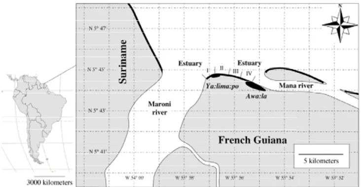
We tested the developed method using an incomplete leatherback nest count dataset (2002) on Ya:lima:po nest-ing beach in French Guiana (Figure 1), and tested it usnest-ing a complete nest count dataset from 1987.
Results
Ya:lima:po entire beach – 2002 data (Table 1)
A total of 3356 nests were counted during 171 field days from 1/3/2002 until 31/12/2002 on the Ya:lima:po nest-ing beach. The Akaike Information Content (AIC) of the 8 models describing the shape of the nesting season was lowest when the K1 parameter was fixed to 0. However, the various model combinations with K1 = 0 and/or K2 = 0 had essentially the same support (i.e. Akaike weights were similar). In contrast, the models with the min parameter fixed to 0 showed considerable lower support. As outlined above, our initial model selection criteria were a) low AIC value and b) fewer parameters. From this, the initial model we retained used 9 parameters (S1, P1, S2, P2, Min,
Max, a, b, c). The goodness of fit for this model was r2 =
0.85 and it estimated a seasonal total of 4652 ± 73SD nests.
We added a sinusoid function to this pattern, by generat-ing a map of -Ln Likelihood with varygenerat-ing φ1 and Δ1 param-eters (Figure 2). The maximum likelihood was observed
Table 1: Model selection for leatherback nest counts on Ya:lima:po beach in 2002. Selected models are in bold.
Models rank by AIC -Ln L Parameters AIC Akaike weights Nests & SD
A: No sinusoid Intra Inter
S1 P1 S2 P2 K2 Max Min 471.31 10 962.63 0.3393 S1 P1 K1 S2 P2 Max Min 471.61 10 963.22 0.2525 S1 P1 S2 P2 Max Min 472.60 9 963.22 0.2520 0.0000 4652 SD 73 S1 P1 K1 S2 P2 K2 Max Min 471.16 11 964.32 0.1454 S1 P1 S2 P2 Max 477.79 8 971.57 0.0039 S1 P1 K1 S2 P2 Max 476.80 9 971.61 0.0038 S1 P1 S2 P2 K2 Max 477.59 9 973.18 0.0017 S1 P1 K1 S2 P2 K2 Max 476.79 10 973.58 0.0014 B: One sinusoid Δ1 φ1 β1 458.32 12 940.65 0.3413 Δ1 φ1 α1 β1 457.52 13 941.05 0.2793 0.0005 4719 SD 62 Δ1 φ1 τ1 β1 457.57 13 941.14 0.2674 Δ1 φ1τ1 α1 β1 457.45 14 942.90 0.1105 Δ1 φ1 α1 463.76 12 951.52 0.0015 C: Two sinusoids Δ2 φ2 α2 β2 449.21 16 930.54 0.6065 0.0864 4716 SD 58 Δ2 φ2 τ2 α2 β2 449.07 17 932.14 0.2730 Δ2 φ2 β2 452.84 15 935.69 0.0463 Δ2 φ2 α2 452.93 15 935.87 0.0423 Δ2 φ2 τ2 β2 452.21 16 936.42 0.0320 D: Three sinusoids Δ3 φ3 α3 β3 441.91 20 923.822 0.3994 Δ3 φ3 β3 442.95 19 923.900 0.3842 0.9132 Δ3 φ3 τ3 α3 β3 441.91 21 925.822 0.1469 Δ3 φ3 τ3 β3 444.27 20 928.550 0.0376 Δ3 φ3 α3 445.44 19 928.878 0.0319
Map of Ya:lima:po beach within the estuary of the Maroni and Mana rivers
Figure 1
Map of Ya:lima:po beach within the estuary of the Maroni and Mana rivers. Nesting beach sections used in this study are indicated in bold.
for φ1 = 9.5 and Δ1 = 6.75. These values were used as initial points to search for values of α1,β1, φ1, Δ1, and τ1
parame-ters that also maximized likelihood. We then searched for a simpler model assuming α1 = 0 and/or β1 = 0 and/or τ1
= l. The model with lowest AIC had a fitted value of τ1. However, based on Akaike weights, this model exhibited a goodness of fit similar to the model with τ1 = 0 (0.50 vs.
0.49). As this latter model was simpler, we retained it for further tests. When one sinusoid was added, the AIC = 940.65, much lower than AIC = 963.22 prior to the addi-tion of the sinusoid. The goodness of fit for this model was r2 = 0.87 and the total number of nests is estimated to
be 4719 ± 62SD.
A second sinusoid was added using the same procedure. The map of -Ln Likelihood showed a minimum for (φ1 = 14 and Δ1 = 4. These values were used as initial points to search for values of α2, β2, φ2, Δ2, and τ2 parameters that
maximized likelihood. Then, we searched for a simpler model by assuming α2 = 0 and/or β2 = 0 and/or τ2 = l. The
model with the lowest AIC value assumed that τ2 = l. When the second sinusoid was added, the AIC = 930.54 and was lower than the AIC obtained with one sinusoid (AIC = 940.65). The goodness of fit for this two-sinusoid model was r2 = 0.88 and the total number of nests it
esti-mated was 4716 ± 58SD (Figure 3). The addition of a third
sinusoid gave the model lower a AIC (923.90), but based on Akaike weight the overall fit was not significantly bet-ter than the model with only two sinusoids. Therefore, the best-fit model based on both AIC and Akaike weight crite-ria had two sinusoids.
Analysis of beach sections – 2002 data
Nest distribution for each beach section (Figure 1) was fit-ted as previously described. A homogeneity test showed that the global shape of nesting was significantly different for the four beach sections (LRT = 391.65, DF = 18, p < 0.0001). A similar conclusion was obtained when only the beginning of the nesting season was assumed to be Leatherback nest distribution during the 1987 and 2002 nest-ing seasons in Ya:lima:po nestnest-ing beach
Figure 3
Leatherback nest distribution during the 1987 and 2002 nest-ing seasons in Ya:lima:po nestnest-ing beach. Black points are the nest counts. The central curve is the best fitted model and the upper and lower curves are the error envelopes (±2 SD). The vertical bars represent, from right to left, d+10%, d+25%, d+50%, day at peak, d-50%, d-25%, d-10% values (see text). -Ln L is -logarithm of maximum likelihood for the cor-responding model and AIC is the Akaike Information Con-tent.
Number of nests per night
M A M J J A S O N D 0 10 20 30 40 50 60 70 80 90 100
2002
-Ln L=449.21 AIC=930.54 r2=0.88 Nests=4716 SD 58 0 100 200 300 400 500 600 700 800Number of nests per night
1987
-Ln L=829.32 AIC=1692.65 r2=0.86 Nests=33424 SD 40 M A M J J A S O N DMap of -Ln Likelihood with varying φ1 and Δ1 parameters for 2002 nesting season
Figure 2
Map of-Ln Likelihood with varying φ1 and Δ1 parameters for 2002 nesting season. 5 6 7 8 9 10 11 12 13 14 15 16 5 6 7 8 4 0 1 2 3 1 475 460 -Ln L 1
identical (LRT = 67.23, DF = 9, p < 0.0001) or the end of nesting season was assumed to be identical (LRT = 294.27, DF = 9, p < 0.0001). The index d+10% that describes the beginning of the nesting season showed a significant spa-tial tendency, with the nesting season beginning later in the western section of the beach (Kendall rank correla-tion, p = 0.04), but no spatial influence was observed for either the peak of the season or the d-10% descriptor of the end of the nesting season (p > 0.05).
Although the shapes of nest distribution among the differ-ent beach sections were significantly differdiffer-ent, the use of a single model for the global shape of nest distribution dur-ing the nestdur-ing season did not affect the estimates of total nest numbers for each zone (Figure 4).
When one sinusoid with a period varying from 5 to 16 days by steps of 0.25 days was added to the models, the beach sections also showed strong differences. Indeed, the sinusoidal period appeared to be different according to the position of the beach section analyzed. The 14.25-days signal was significantly strong within section I whereas the 9.8-days signal was significantly strong within section IV (Figure 5).
Ya:lima:po entire beach – 1987 data (Table 2)
A total of 33337 nests were counted during 178 field days from 1/3/1987 until 15/9/1987 on Ya:lima:po nesting beach. Only 22 daily counts were missing at the end of the nesting season. This time-series can therefore be
consid-ered as essentially complete as the nesting after July is rel-atively sparse. The AIC of the 8 models describing the overall shape of nesting season was lowest when the K1
parameter was fixed to 0, but was not significantly differ-ent from several other models based on Akaike weight (Table 2A). We choose the first one in the series with Akaike weight > 0.05 and minimum number of fitted parameters.
We added a sinusoid function to this pattern, by generat-ing a map of -Ln Likelihood with varygenerat-ing φ1 and Δ1
param-Likelihood for nest distributions on the different beach sec-tions when one sinusoid with varying period was added Figure 5
Likelihood for nest distributions on the different beach sec-tions when one sinusoid with varying period was added. The dashed line defined the limit of -Ln L statistical significance using Akaike weight after applying a Bonferronni correction for multiple tests.
Section I
Section II
Section III
Section IV
1in days
-Ln L
254 256 258 260 262 264 266 268 270 272 274 5 6 7 8 9 10 11 12 13 14 15 16 430 432 434 436 438 440 442 5 6 7 8 9 10 11 12 13 14 15 16 88 90 92 94 96 98 100 102 104 106 5 6 7 8 9 10 11 12 13 14 15 16 372 373 374 375 376 377 378 379 380 381 382 5 6 7 8 9 10 11 12 13 14 15 16Estimated nest numbers for various beach sections if each beach section was fitted using its own model (4 different models, open bars) or if a single fitted model was used for all beach sections (1 single model, closed bars)
Figure 4
Estimated nest numbers for various beach sections if each beach section was fitted using its own model (4 different models, open bars) or if a single fitted model was used for all beach sections (1 single model, closed bars).
0 1000 2000 3000 4000 5000
Section I Section II Section III Section IV Total
Shape of nesting season fitted individually for each section Shape of nesting season fitted once for all sections
Number of nests
eters. The maximum likelihood was observed for (φ1 =
15.25 and Δ1 = ll. These values were used as initial points to search for values of the α1, β1, φ1, Δ1 and τ1 parameters that maximized likelihood. We then searched for a sim-pler model assuming α1 = 0 and/or β1 = 0 and/or τ1 = 1 (Table 2A). The model with the lowest AIC had a nearly identical AIC value to the model that was had one less parameter (τ1 was set to 1). Using the principle of parsi-mony, we retained the model with fewer parameters for further exploration. Second and third sinusoidal signals were added to the model; we selected the single model within all groups of models (0, 1, 2, or 3 sinusoidal sig-nals added) with the lowest AIC values. Of these four, we found that the model with 2 sinusoidal signals had the lowest Akaike weight (Table 2). The two sinusoidal peri-ods fitted were 10.60 and 15.34 days. The Gratiot et al. model [19] when applied to this time-series was strongly rejected compared to the model presented here (AIC 2047.30 vs. 1693.67; p < 10-10 based on Akaike weight).
The number of observed nests during the 178 night
patrols was 33337. The number of nests calculated by the models was as follows: 33223 (ε = -0.34%) for no sinusoi-dal signal, 33305 (ε = -0.09%) for 1 sinusoidal signal added, and 33118 (ε = -0.65%) for 2 sinusoidal signals added (Figure 3). All three estimates are close to the observed number of nests (note that the number of nests reported in Table 2 are for the entire nesting season, including the final 22 days without available nest counts). The periodic signal within number of nests that was detected in the 1987 database comprised of 161 consecu-tive day counts can be also tested using classical mathe-matical tools. The Multi-Taper method (MTM) of spectral analysis provides a means for spectral estimation [20,21] of a time series that is believed to exhibit a spectrum con-taining both continuous and singular components. A MTM test for white noise in this time-series indeed detects a significant period signal at both 10.60 days (p < 0.01) and at 15.34 days (p < 0.05). However, the MTM method can be used only with continuous time-series, which
Table 2: Model selection for leatherback nest counts on Ya:lima:po beach in 1987. Selected models are in bold.
Model ranked by AIC -Ln L Parameters AIC Akaike Weights Nests & SD
A: No sinusoid Intra Inter
S1 P1 K1 S2 P2 Max Min 857.26 10 1734.53 0.3551 S1 P1 S2 P2 K2 Max 858.92 9 1735.84 0.1847 0.0000 33563 SD 44 S1 P1 K1 S2 P2 Max 859.20 9 1736.41 0.1392 S1 P1 K1 S2 P2 K2 Max Min 857.26 11 1736.54 0.1306 S1 P1 K1 S2 P2 K2 Max 858.56 10 1737.13 0.0972 S1 P1 S2 P2 K2 Max Min 858.94 10 1737.90 0.0661 S1 P1 S2 P2 Max Min 860.92 9 1739.85 0.0249 S1 P1 S2 P2 Max 864.34 8 1744.69 0.0022 B: One sinusoid Δ1 φ1 τ1 α1 β1 844.89 14 1717.79 0.4755 Δ1 φ1 α1 β1 845.94 13 1717.90 0.4494 0.0000 33624 SD 49 Δ1 φ1 α1 848.78 12 1721.56 0.0722 Δ1 φ1 β1 852.30 12 1728.61 0.0021 Δ1 φ1τ1 β1 852.32 13 1730.64 0.0008 C: Two sinusoids Δ2 φ2 τ2 α2 β2 828.43 18 1692.86 0.5988 Δ2 φ2 α2 β2 829.83 17 1693.67 0.3992 0.1168 33424 SD 40 Δ2 φ2 α2 836.10 16 1704.20 0.0021 Δ2 φ2 τ2 β2 841.28 17 1716.56 0.0000 Δ2 φ2 β2 842.35 16 1716.71 0.0000 D: Three sinusoids Δ3 φ3 τ3 β3 823.81 21 1689.63 0.4555 0.8832 Δ3 φ3 α3 β3 824.47 21 1690.94 0.2370 Δ3 φ3 τ3 α3 β3 823.80 22 1691.60 0.1704 Δ3 φ3 τ3 β3 826.21 20 1692.42 0.1129 Δ3 φ3 α3 827.74 20 1695.49 0.0243
therefore makes it ineffective when analyzing marine tur-tle datasets that contain gaps in coverage.
Discussion
The total number of nests deposited during the nesting season is often used as an index of abundance for marine turtle species. To obtain reliable data, monitoring of the nesting beach should be conducted on a regular basis dur-ing the nestdur-ing season. However, nestdur-ing seasons can span up 6 months or more, making it challenging to effectively collect data on a daily basis [12]. It is common for nesting beach datasets to be missing information, either during, at the beginning and/or at end of the nesting season. One means to account for data gaps during the nesting season is to employ interpolation. For instance, Girondot & Fretey [16] were able to fill in data gaps for a leatherback nesting population using interpolation with a small asso-ciated error (5%). However, this procedure is inadequate if the beginning and/or the end of a nesting season is not monitored. Troëng et al. [8] used a moving average, but again, the behavior of such a function can be erratic at the boundaries of the time-series. Yet gaps at the beginning or end of the season are common because research teams tend to concentrate monitoring effort at the peak of the nesting season. To be able to extrapolate data, one needs an equation that accurately describes the global nesting season. A recently proposed symmetrical model of a leath-erback nesting season [19] is inadequate for modeling the dataset from Ya:lima:po because the time series analyzed above was not symmetrical (for example, based on the 2002 time-series: symmetric model with S1 = S2 and (K1 =
K2) ≠ 0 AIC 966.26 or S1 = S2 and K1 = K2 = 0 AIC 964.51 vs. asymmetrical model – see Table 1B – S1 ≠ S2 and K1 = K2 = 0 AIC 963.22). Also, nest counts outside the main sinusoid were calculated separately before the fitting pro-cedure used by Gratiot et al. [19]. Finally, a fitting proce-dure based on two rounds should be avoided, as they generally do not converge on the best fit of the data. In contrast, we have shown that the best fit model describ-ing the nestdescrib-ing season of leatherback at Ya:lima:po exhib-its three components: an overall shape describing the nesting season and two sinusoids signals. For 1987, one signal has a period of 10.60 ± 0.0003 SD days and the other a period of 15.34 ± 0.0004 SD days. For 2002, one signal has a period of 9.74 ± 0.01 SD days and the other a period of 14.11 ± 0.004 SD days. The first signal likely rep-resents the reproductive cycle of females that nest sequen-tially during the nesting season, with nests separated by approximately nine to ten days [16]. The second signal could be related to the lunar or tidal phase when full and new moon alternate every 14.25 days [16]. This signal was particularly strong for the beach section located furthest within the estuary (Section I, Figure 5). In this section, the peak of nesting coincided with the spring high tides
observed during each full and new moons. Interestingly, it has been observed that greater numbers of female leath-erbacks become trapped in exposed mud flats after nest-ing durnest-ing neap tides on the nearby beaches in Suriname [22]. However, we do not think that the peak of nesting during spring tides represents a selective avoidance response to this potential mortality factor, for the follow-ing two reasons. First, the actual mortality rate is low for females that are temporarily trapped in the mud-flats (M.G., personal observation), making it unlikely that this would constitute a strong selective pressure. Second, the peak of nesting during spring tide is not observed in all beach sections (Figure 4). Nesting at high tide during spring tide could be also viewed as a way to minimize energy expenditure while selecting a suitable site for nest-ing on the beach [23]. Alternatively, the peaks in nestnest-ing distribution at spring high tide could result from currents in the Maroni river that may prevent individual leather-backs from nesting too far inside the estuary at neap tide (Figure 1). However, an expected complementary peak at neap tide in other beach sections further away from the Maroni was not detected (Figure 5). A third possible explanation is that a shift of female turtles from other nesting beaches in the region (Figure 1) to Ya:lima:po beach may be associated with the spring high tide. Cur-rent data are insufficient to test this hypothesis.
In French Guiana, leatherback females can adjust their return nesting date from 6 to 16 days between two nesting events in order to be closer to a full or new moon [16]. This effect was not observed in leatherbacks nesting on the Pacific coast of Costa Rica [24]. However, the number of observations available from Costa Rica was only one tenth of the number in Girondot & Fretey [16], which is insuffi-cient to detect an effect similar to the one observed in Ya:lima:po (M.G., unpublished results). Note that even with this significant peak of nesting at the spring high tide, leatherbacks in French Guiana have a stronger signature at 9.8 days that is the characteristic nesting interval for this species [25]. Stronger and more significant periodic sig-nals were detected at both ends of the Ya:lima:po nesting beach (Sections I and IV, Figure 5). The lack of significant signal in sections II and III is probably the consequence of reduced environmental constraints from tide or river cur-rents for the central sections of the beach.
The numbers of total nests calculated by the various meth-ods proposed here were not significantly different: the additions of one or two sinusoidal signals in 2002 changed the estimation of total nest number from 4652 ± 73 SD (no sinusoids), to 4719 ± 62 SD (one sinusoid) and 4716 ± 58 SD (two sinusoids). Given the consistency of total nest estimates, one could question why a more com-plex model is needed. It should be noted that the standard deviations of the estimates were lower with the addition
of sinusoids because these sinusoids explained some of the variation that was expressed by the standard deviation of the simpler models (Figure 6). Therefore, the beta risk was reduced when the estimate was derived with the more complex model.
Conclusion
The model proposed here offers a variety of uses beyond its application in accurately estimating total counts from an incomplete dataset. It also can detect intraseasonal concentrations of animals that may be the result of behav-ioral interactions, synchronization with external factors and/or biological constraints. When applied to leather-backs nesting in French Guiana, the model detected 3 principal components that contribute to the seasonal nest distribution: a global shape that corresponds to the arrival and departure of leatherback females in the Guianas region, a sinusoidal pattern with a period of approxi-mately 10 days that is related to physiological constraints of nesting leatherbacks, and a sinusoidal pattern with a longer period that likely reflects the influence of the spring high tide on nesting turtles.
The proposed model is an improvement over previously published methods [8,16,19] but we should keep in mind that nest number is only an index of the population size. Indeed, variable remigration interval [26] and variable number of nest per female [15] affect also strongly the observed number of nests for a particular year.
Methods
Nesting dataNest count data were collected in 1987 and 2002 on Ya:lima:po nesting beach in French Guiana (Figure 1). This nesting beach is approximately 4 km long and was divided into 4 sections that were roughly equal in dis-tance. Nesting activity of leatherback turtles was moni-tored either by conducting daily dawn patrols to count all nest tracks made the previous night and/or by counting individual nesting females at night when total nests per night > 50 [see complete description in [27]]. False crawls are relatively rare in leatherbacks nesting in French Guiana and only tracks that reach the upper part of the beach and had signs of post-oviposition camouflaging by the female turtle were counted as nests. Nest counts were made during the primary nesting season, from 1st March (defined as day 0) until 15 September 1987 or 31 Decem-ber 2002. Data for January and February were not included because leatherbacks display a smaller second-ary nesting season during these months [28]. In 1987,178 nights from 1/3/1987 until 15/9/1987 were worked on the Ya:lima:po nesting beach. Only 22 daily counts were missing at the end of the nesting season (10/8/1987 to 31/8/1987). This time-series can be considered as nearly complete as the nesting after July is relatively rare. A total of 33337 nests were counted during the 1987 season. Of the 305 days of the 2002 primary nesting season, 3356 nests were counted on 171 nights (56% coverage). Whether observed at night or the following morning, each nest was assigned the date prior to midnight of the night it was laid. The lunar phase for each night was also calcu-lated using internet moon phase calculator [29].
The model to describe the nesting season
Nesting seasons of marine turtles are typically character-ized by a peak of nesting approximately during the middle of the nesting season. The number of nests at the start and end of the nesting season is low ; generally less than one nest per week or per month in some populations (unpub-lished data). This typical pattern has been modeled as a sinusoid function [19]. However, this function presup-poses that the shape of the seasonal nesting distribution is symmetrical. Several different populations of marine tur-tles display asymmetrical peaked patterns associated with their nesting season [e.g. [30-32]]. Moreover, the assump-tion that the temporal nesting distribuassump-tion of sea turtles is a simple sinusoid has several inherent statistical weak-nesses (see below).
As an alternative, the seasonal nesting pattern can be modeled using the product of two sigmoid equations, the first one ranging from 0 to 1 and the second one from 1 to 0. The product shows a 0-1-0 pattern if the transition of the first equation is observed at an abscissa of lower value than the second one. For each sigmoid equation, we use a Standard deviations of the fitted model with zero, one or
two sinusoids added to the global pattern Figure 6
Standard deviations of the fitted model with zero, one or two sinusoids added to the global pattern.
No sinusoid
One sinusoid
Two sinusoids
Nest count for a night Fitted standard deviation model for a night
0 10 20 30 40 50 60 70 0 50 100 150 200
modified form of the Verhulst equation [33] that allows asymmetry to be set. Note that the first-order derivative of this equation is similar to the Richards equation [34]:
where d is the Julian date, P is related to the dates before and after the peak nesting day when there is an observed maximum rate of change (increase or decrease) in nest numbers, and S and K are related to the change in slope of the change in nest numbers at date P.
The value of M(d) ranges from 0 to 1 with M(d) = 0.5 for
P = d, with d being the number of days since the start of
the nesting season. The steepness of M(d) at P = d depends on S and K values. M(d) is increasing when S is negative (i.e. at the start of the nesting season) and decreasing when S is positive (i.e. at the end of nesting season). Asymmetry around P is determined by a positive or nega-tive value of K. The equation (1) is reduced to a simple logistic equation (i.e. symmetrical around P) when K = 0. To avoid a computing overflow, the equation (1) was sim-plified to
when
and to when K > 3 and sign(P-d) = sign(S).
The mathematical description of a nesting season can therefore be expressed as:
N(d) = min + (max - min) · (M1 (d) · M2 (d)) (2) with M1(d) and M2(d) being the first and second halves of the nesting season, respectively. The difference between the two largely rests on the sign of the S parameter: S1 is negative, S2 is positive and P1 <P2. The parameter min is
the basal level of nesting outside the nesting season and
max-min is a scaling factor. Note that max is not the
maxi-mum of the function because (M1(d) · M2 (d)) can be lower than 1 at the peak of nesting season. The maximum must be calculated numerically.
The entire nesting season can be expressed using equation (2), which is based on 8 parameters. The number of parameters can be reduced using the Verhulst equation around P1 (K1 = 0), P2 (K2 = 0), or both. The basal level of nests min can be fixed to 0. Also, if it is assumed that the
beginning and the end of nesting season show similar shapes, this can be expressed by setting S1 = -S2 and K1 =
K2. The most reduced form of equation 2 uses only 4 parameters (min = 0, K1 = K2 = 0, S1 = -S2). The test for an asymmetrical shape of the nesting season was performed by forcing S2 = -S1 and K1 = K2.
Equation (2) describes the global shape of the nesting sea-son. A more complete model could also incorporate peri-odic variation within the nesting season. Traditionally, spectral analysis has been used to describe periodic pat-terns, but the discontinuities in the daily nest count data-set makes the use of these tools inappropriate [35]. Instead, a sinusoid function was incorporated into the equation (2) and the corresponding parameters are fitted against the daily nest counts. When several periodic sig-nals were detected, the sum of/sinusoid equations was used:
Parameter φ defines the period of the sinusoidal pattern and Δ is the phase shift. The amplitude of variation is gov-erned by α, β and τ parameters. If the amplitude is inde-pendent of the number of nests, then α ≠ 0 and β = 0 (the parameter τ is not used and set to 1). If α ≠ 0 and β ≠ 0, then the amplitude(s) of the fluctuations have two com-ponents, one dependent and one independent of the number of nests. The parameter τ ≠ l renders a non-linear dependent relationship between amplitude of the fluctu-ations and number of nests. Equation (3) implies that sinusoid signals are additive. It can be changed to allow a multiplicative effect but this kind of model performs less well than the additive model and will not be discussed further (data not shown). The model defined with equa-tion (3) uses 5l parameters more than the model defined with equation (2). Equation (3) can be simplified setting α = 0 or β = 0 and/or τ = l (3 or 4 parameters).
The curve was fitted to experimental data by maximum likelihood method using a simplex search [36] followed by a gradient search [37]. For this purpose, we assumed that the nest distribution for day d is normally distributed with a standard deviation σa = Exp(a.N'(d)c + b) where a, b and c are parameters that are also fitted. This function has the advantage of being strictly positive and monotonically increasing according to N'(d) when a and c are positive. It also accounts for the observed heteroskedasticity, i.e. nest counts were more dispersed at the peak of nesting season. An alternative is to use the lognormal distribution for nest number which has the advantage of being always positive but also requires a forced origin that is not zero as zero nests is not a possible output.
M d e e S P d e K K ( ) ( ) / = + −
(
)
⎛ ⎝ ⎜ ⎞ ⎠ ⎟ ( ) − ⎛ ⎝⎜ ⎞ ⎠⎟ − 1 2 1 1 1 1 M d e eK e eK S P d ( ) / ( ) = −(
−)
⎛ ⎝ ⎜ ⎞ ⎠ ⎟ − ⎛ ⎝⎜ ⎞⎠⎟ 1 2 1 1 2 1 1 e S P d K e −(
)
⎛⎝⎜ ( − )⎞⎠⎟ 1 2e d P SeK − ⎛ ⎝⎜ ⎞ ⎠⎟ ′ = + ⎛ + ⎝ ⎜ ⎞⎠⎟(
+ ⋅)
⎛ ⎝ ⎜⎜ ⎞⎠⎟⎟ ( ) =∑
N d N d d k N d k k k k l k ( ) ( ) sin 2 ( ) 3 1 π φ α β τ ΔFor ease of use, this modeling application has been scripted for both MacOS and Microsoft Windows plat-forms [38].
Model selection and goodness of fit
Model selection was performed using the Akaike Informa-tion Content [39]. This is a ranking measure that takes into account the quality of the fit of the model to the data while penalizing for the number of parameters used: AIC = -2 In L + 2 M (4)
where L = maximum likelihood, and M = the number of parameters. The models with the lowest values of AIC were retained as good candidate models and ΔAIC was
cal-culated as the difference in value of AIC between a partic-ular model and the one with the lowest AIC. Akaike weights (wi = exp(-ΔAIC/2) normalized to 1) were used to evaluate the relative support of various tested models [40]. Akaike weights can be directly interpreted as condi-tional probabilities for each model. Ideally, the model with the lowest AIC was kept for further testing. When two or more models possessed similar Akaike weights, the model with the lowest number of parameters was selected. When several of these models had the same number of parameters, the model with the lowest AIC among them was selected.
When varying the period of sinusoid signal within the nesting season, the significance levels of the models with or without sinusoidal signals were tested using Akaike weight after a Bonferronni correction. Let L0 be the -Ln likelihood of the best model without a sinusoid and let B be a matrix of b -Ln likelihoods (b is the Bonferronni cor-rection factor) obtained by varying φ1 parameter and fit-ting β1 and Δ1. A likelihood i of the B matrix was considered as being significantly better than L0 if wi < 0.05/b. Therefore, a model with a sinusoid was signifi-cantly better (p < 0.05) than the model without one if the difference between likelihoods was higher than
.
Goodness of fit was evaluated using the coefficient of determination (r2) between the observed and estimated
nest numbers to facilitate comparisons with a previously published method [19]. However, it is important to note that the r2 statistic is inadequate for non-stationary
time-series such as those analyzed here, as any distribution showing a peak at the middle of the time-series will gen-erate an inflated r2 value.
For the model being fitted, the error ε in per cent on the estimate of the total number of nests was calculated as [19]:
with n(t) being the observed number of nests for night t.
Note that this formula assumes that nest counts are known for each day of the time series, which is rarely the case and only days with known nest counts were used to calculate ε.
The standard error for the parameters was estimated using a standard procedure to estimate the variance of a func-tion about a point [41]. In short, when applied to the error in the location of one point this procedure is directly related to the uncertainty in the model relative to the posi-tion of the peak (mathematically represented by the standard error in the estimation of the point where the first derivative is zero). It is inversely related to the value of the second derivative about the maximum. It is approx-imated using a fourth order polynomial function around the fitted value for each parameter [41].
Synthetic parameters
Not all parameters involved in equation (2) could be directly derived to describe aspects of nesting season (beginning, end, or length) because of complex interac-tions between them. Rather, several new statistics were calculated. The d+x% and d-x% values are the days where
N(d) is equal to x% of the maximum nest number (d+
indicates the start of nesting season and d- the end of nest-ing season with x = 10, 25 and 50%). The values d+x% and d-x% are an index that is proportional to the begin-ning and the end of nesting season. The value d-x% – d+x% is an index related to the length of the nesting sea-son. Equation (2) cannot be transformed to directly obtain the d ± x% values, rather a numerical approxima-tion was required. The standard errors for the d ± x% val-ues were obtained by 100 replications of equation (2) with parameter values obtained randomly from values that maximized the likelihood while taking into account the standard error. The total number of nests deposited during the entire season was the sum of the number of nests laid per night.
Homogeneity test
The test for homogeneity of the nest distribution for sev-eral nesting beaches was performed using likelihood ratio test and AIC comparison. We assumed that Li was the maximum likelihood and Mi was the number of parame-ters for beach section i. Under the hypothesis that nest dis-tribution was the same for all these nesting beach sections,
2 0 05 1 0 05 + −
(
)
⎛ ⎝ ⎜ ⎞ ⎠ ⎟ ln . / . / b b ε =⎛ ′ − ⎝ ⎜⎜ ⎞ ⎠ ⎟⎟ = =∑
=∑
N t n t∑
n t t t t ( ) ( ) ( ) 1 365 1 365 1 365a single common set of parameters could be calculated. Some parameters may be allowed to vary in specific cir-cumstances, for example max and min might vary to take into account that, on various beach sections, the total number of nests laid can be different. When k nesting beach sections are compared, the likelihood of these k sec-tions analyzed with a single set of M parameters is L. The statistic -2 In (∏ Li/L) is distributed as a χ2 with M-ΣM
i
degrees of freedom.
Authors' contributions
MG initiated this project and conducted most of the anal-yses. PR refined some hypothesis and conducted some analyses. JPB helped with statistics and conducted some analyses. MHG refined some hypotheses and headed fieldwork. RW headed fieldwork. VH, EG and SC helped collect field data.
Acknowledgements
Many individuals from the different organizations involved in marine turtle field work in French Guiana have helped collect the data used in this study: Kulalashi from the villages of Ya:lima:po and Awa:la, Eric Hansen and Johan Chevalier (Office National de la Chasse et de la Faune Sauvage), the Réserve Naturelle de 1'Amana, and the Syndicat Intercommunal à Vocation Unique de 1'Amana. Financial support was provided by the Direction Régionale de I'Environnement Guyane, the Ministère de 1'Ecologie et du Développement Durable, Créocéan and Hardman Resources LTD. This paper greatly benefited from the comments of three referees.
References
1. Alerstam T: Bird migration Cambridge, UK: Cambridge University Press; 1990.
2. Berthold P: Control of bird migration London, UK: Chapman and Hall; 1996.
3. Burdick HC: A marked migration wave during the 1943 spring
season. Bird-Banding 1943, 14:131-133.
4. Winker K, Escalante P, Rappole JH, Ramos MA, Oehlenschlager RJ, Warner DW: Periodic migration and lowland forest refugia in
a "sedentary" neotropical bird, Wetmore's bush-tanager.
Conservation Biology 1997, 11:692-697.
5. Byrd GV, Day RH, Knudtson EP: Pattern of colony attendance
and censusing of auklets at Buldir Island, Alaska. Condor 1983, 85:274-280.
6. James MC, Eckert SA, Myers RA: Migratory and reproductive
movements of male leatherback turtles (Dermochelys coria-cea). Marine Biology 2005, 147:845-853.
7. Gerrodette T, Taylor BL: Estimating population size. In Research and management techniques for the conservation of sea turtles Edited by: Eckert KL, Bjorndal KA, Abreu-Grobois FA, Donnelly M. IUCN/SSC Marine Turtle Specialist Group Publication No. 4; 1999:67-71. 8. Troëng S, Chacón D, Dick B: Possible decline in leatherback
tur-tle Dermochelys coriacea nesting along the coast of Carib-bean Central America. Oryx 2004, 38:395-403.
9. Bolten AB, Witherington BE: Loggerhead Sea Turtles Washington, D.C.: Smithsonian Books; 2003.
10. Schroeder B, Murphy S: Population surveys (ground and aerial)
on nesting beaches. In Research and Management Techniques for the
Conservation of Sea Turtles Edited by: Eckert KL, Bjorndal KA, Abreu-Grobois FA, Donnelly M. IUCN/SSC Marine Turtle Specialist Group Publication No. 4; 1999:45-55.
11. Gates CE, Valverde RA, Mo CL, Chaves AC, Ballesteros J, Peskin J:
Estimating arribada size using a modified instantaneous count procedure. Journal of Agricultural Biological and Environmental
Statistics 1996, 1:275-287.
12. Kerr R, Richardson JI, Richardson TH: Estimating the annual size
of hawksbill (Eretmochelys imbricatd) nesting populations
from mark-recapture studies: the use for long-term data to provide statistics for optimizing survey effort. Chelonian
Con-servation and Biology 1999, 3:251-256.
13. Marquez MR, Van Dissel HG: A method for evaluating the
number of massed nesting olive ridley sea turtles, Lepidoche-lys olivacea, during an arribazon, with comments on arriba-zon behaviour. Netherlands Journal of Zoology 1982, 32:419-425.
14. Buckland ST, Anderson DR, Burnham KP, Laake JL: Distance sampling: Estimating abundance of biological populations London, UK: Chapman & Hall; 1993.
15. Rivalan P, Pradel R, Choquet R, Girondot M, Prévot-Julliard A-C:
Estimating clutch frequency in marine turtles through stop-over duration. Marine Ecology-Progress Series 2006 in press.
16. Girondot M, Fretey J: Leatherback turtles, Dermochelys
coria-cea, nesting in French Guiana, 1978–1995. Chelonian Conserva-tion and Biology 1996, 2:204-208.
17. Kalb H: Behavior and physiology of solitary and arribada
nest-ing Olive Ridley sea turtles (Lepidochelys olivacea) durnest-ing the internesting period. In Ph.D. Dissertation Texas A&M University,
College Station; 1999.
18. Sato K, Matsuzawa Y, Tanaka H, Bando T, Minamikawa S, Sakamoto W, Naito Y: Internesting intervals of loggerhead turtles,
Caretta caretta, and green turtles, Chelonia mydas, are affected by temperature. Canadian Journal of Zoology 1998, 76:1651-1662.
19. Gratiot N, Gratiot J, de Thoisy B, Kelle L: Estimation of marine
turtles nesting season from incomplete data; statistical adjustment of a sinusoidal function. Animal Conservation 2006, 9:95-102.
20. Thomson DJ: Spectrum estimation and harmonic analysis. Pro-ceedings IEEE 1982, 70:1055-1096.
21. Percival DB, Walden AT: Spectral analysis for physical applications Cam-bridge, UK: Cambridge University Press; 1993.
22. Hilterman M, Goverse E: Annual Report on the 2003
Leather-back Turtle Research and Monitoring Project in Suriname.
Guianas forests & environmental conservation project 2004:25. 23. Mrosovsky N: Ecology and nest-site selection of leatherback
turtles Dermochelys coriacea. Biological Conservation 1983, 26:47-56.
24. Lux J, Reina R, Stokes L: Nesting activity of leatherback turtles
(Dermochelys coriacea) in relation to tidal and lunar cycles at Playa Grande, Costa Rica. In Proceedings of the Twenty-Second
Annual Symposium on Sea Turtle Biology and Conservation Miami FL Edited by: Seminoff JA. NOAA Technical Memorandum NMFS-SEFSC-503; 2003:215-216.
25. Reina RD, Mayor PA, Spotila JR, Piedra R, Paladino FV: Nesting
Ecol-ogy of the Leatherback Turtle, Dermochelys coriacea, at Parque Nacional Marino Las Baulas, Costa Rica: 1988–1989 to 1999–2000. Copeia 2002, 2002:653-664.
26. Hays GC: The implications of variable remigration intervals
for the assessment of population size in marine turtles.
Jour-nal of Theoretical Biology 2000, 206:221-227.
27. Chevalier J, Girondot M: Dynamique de pontes des Tortues
luths en Guyane française durant la saison 1997. Bull Soc Herp
Fr 1998, 85–86:5-19.
28. Chevalier J, Talvy G, Lieutenant S, Lochon S, Girondot M: Study of
a bimodal nesting season for leatherback turtles (Dermoche-lys coriacea) in French Guiana. In 19th Annual Symposium on Sea Turtle Biology and Conservation; South Padre Island, TX Edited by: Kalb H, Wibbels T. U.S. Dept. Commerce. NOAA Tech. Memo. NMFS-SEFSC-443; 1999:264-267.
29. Moon Phase Calculator [http://stardate.org/nightsky/moon/]
30. Diamond AW: Breeding biology and conservation of hawksbill
turtles, Eretmochelys imbricata L., on Cousin Island, Sey-chelles. Biological Conservation 1976, 9:199-215.
31. Duque VM, Paez VP: Nesting ecology and conservation of the
leatherback turtle, Dermochelys coriacea, at La Playona, Chocoan Gulf of Uraba (Colombia), in 1998. Actualidades
Bio-logicas Medellin 2000, 22:37-53.
32. Steyermark AC, Williams K, Spotila JR, Paladino FV, Rostal DC, Mor-reale SJ, Koberg MT, Arauz R: Nesting leatherback turtles at Las
Baulas National Park, Costa Rica. Chelonian Conservation and
Biol-ogy 1996, 2:173-183.
33. Verhulst PF: Deuxième mémoire sur la loi d'accroissement de
la population. Mémoires de l'Académie Roy ale des Sciences, des Lettres
Publish with BioMed Central and every scientist can read your work free of charge "BioMed Central will be the most significant development for disseminating the results of biomedical researc h in our lifetime."
Sir Paul Nurse, Cancer Research UK
Your research papers will be:
available free of charge to the entire biomedical community peer reviewed and published immediately upon acceptance cited in PubMed and archived on PubMed Central yours — you keep the copyright
Submit your manuscript here:
http://www.biomedcentral.com/info/publishing_adv.asp
BioMedcentral
34. Richards FJ: A flexible growth function for emperical use. Jour-nal of Experimental Botany 1959, 29:290-300.
35. Kirchner JW, Weil A: No fractals in fossils extinction statistics. Nature 1998, 395:337-338.
36. Press WH, Teukolshy SA, Vetterling WT, Flannery BP: Numerical Rec-ipes in C : The Art of Scientific Computing Cambridge, UK: Cambridge University Press; 1992.
37. Greenstadt J: On the relative efficiencies of gradient methods. Mathematics of Computation 1967, 21:360-367.
38. Parametric nest distribution [http://www.ese.u-psud.fr/epc/con
servation/pnd/]
39. Akaike H: A new look at the statistical model identification. Ieee Transactions on Automatic Control 1974, 19:716-723.
40. Burnham KP, Anderson DR: Model selection and inference. A practical information-theoretic approach New York, US: Springer-Verlag; 1998. 41. Rice JA: Mathematical statistics and data analysis Belmont, CA: Duxbury