HAL Id: hal-01847657
https://hal-imt-atlantique.archives-ouvertes.fr/hal-01847657
Submitted on 23 Jul 2018
HAL is a multi-disciplinary open access
archive for the deposit and dissemination of
sci-entific research documents, whether they are
pub-lished or not. The documents may come from
teaching and research institutions in France or
abroad, or from public or private research centers.
L’archive ouverte pluridisciplinaire HAL, est
destinée au dépôt et à la diffusion de documents
scientifiques de niveau recherche, publiés ou non,
émanant des établissements d’enseignement et de
recherche français ou étrangers, des laboratoires
publics ou privés.
Scalable Deterministic Scheduling for WDM Slot
Switching Xhaul with Zero-Jitter
Bogdan Uscumlic, Dominique Chiaroni, Brice Leclerc, Thierry Zami, Annie
Gravey, Philippe Gravey, Michel Morvan, Dominique Barth, Djamel Amar
To cite this version:
Bogdan Uscumlic, Dominique Chiaroni, Brice Leclerc, Thierry Zami, Annie Gravey, et al..
Scal-able Deterministic Scheduling for WDM Slot Switching Xhaul with Zero-Jitter.
2018
Interna-tional Conference on Optical Network Design and Modeling (ONDM), May 2018, Dublin, France.
�10.23919/ONDM.2018.8396114�. �hal-01847657�
Scalable Deterministic Scheduling for WDM Slot
Switching Xhaul with Zero-Jitter
Bogdan Uscumlic
1, Dominique Chiaroni
1, Brice Leclerc
1, Thierry Zami
2, Annie Gravey
3, Philippe Gravey
3, Michel
Morvan
3, Dominique Barth
4and Djamel Amar
31Nokia Bell Labs, Paris Saclay, France, [email protected] 2Nokia, Paris Saclay, France, [email protected]
3IMT Atlantique Bretagne-Pays de la Loire, Brest, France, [email protected] 4DAVID, Université de Versailles Saint-Quentin-en-Yvelines, Versailles, France, [email protected]
Abstract— A low-cost WDM slot switching "N-GREEN"
network is studied for the Xhaul application. We assess the impact of inter-slot intervals on the jitter in N-GREEN and propose a deterministic scheduler ensuring a zero-jitter performance as needed by CPRI traffic. We also propose an integer linear program and a corresponding scalable heuristic and use these tools to evaluate the efficiency of the new scheduler within the N-GREEN technology. The results show important savings and improvements in cost, energy consumption, latency and jitter using N-GREEN w.r.t. state-of-the-art Ethernet Xhaul.
Keywords— 5G; Xhaul; zero-jitter; deterministic scheduling; scalability; WDM slot switching.
I. INTRODUCTION
The Ethernet-based fronthaul scheduling problem has recently become a topic of many research groups. Although Ethernet is a mature technology, Ethernet-based fronthaul exploiting statistical multiplexing has difficulties to support synchronization constraints, low jitter (<65ns) and latency (<100 µs) for the CPRI (Common Public Radio Interface) traffic [1] in this network segment.
Recently, a new WDM slot switching technology called WDM Slotted Add/Drop Multiplexer (WSADM), investigated in the ANR N-GREEN project, has been proposed for the 5G fronthaul/Xhaul networks [2], [3]. The WSADM technology of the N-GREEN project exploits the WDM transparency for the transit traffic to lower the cost of optical components and adopt off-the-shelf devices. The WDM slot technology (in which the data is carried simultaneously over 10 wavelengths [2]) has the potential to provide a low-cost [3] and performant fronthaul/Xhaul. However, the problem of the deterministic scheduling of isochronous (CPRI) traffic over a time slotted ring (such as adopted in N-GREEN), where each time slot starts after a fixed size inter-slot interval (“guard time”, 𝑇𝐺), has not
yet been solved. Furthermore, the scalable scheduling method has not yet been proposed. Indeed, the scalability of the scheduling mechanism is needed to reduce the network reconfiguration time, since the scheduler will be implemented at the SDN (software defined networking) controller, enabling the logically centralized network control.
Our main contributions are as follows. For a first time, the impact of guard time on the jitter performance is considered in the scope of deterministic scheduling. Then, a deterministic scheduler with zero-jitter is proposed for N-GREEN. For this scheduler, a solution is proposed in the form of Integer Linear Program (ILP), enabling to achieve the scheduling at optimal network cost. Next, a heuristic algorithm based on the greedy approach is designed as an alternative scalable solution for the same scheduling. Finally, by using the previously developed tools, we evaluate the cost, jitter and latency advantages of the N-GREEN technology when compared to a state-of-the-art Ethernet Xhaul.
The remainder of the paper is organized as follows. In Section II we present the N-GREEN network and node architecture and define the properties of the WDM transponders (WDM-TRX) used for the network operation. Section III defines the scheduling solution that we propose for the WDM slot switching Xhaul network. In Section IV, we detail the mathematical model (based on ILP) implementing the previous scheduling algorithm. Section V introduces the greedy algorithm for the scalable scheduling, while Section VI provides detailed numerical results, evaluating the cost and the power consumption of the N-GREEN network. Finally, concluding remarks are provided in Section VII.
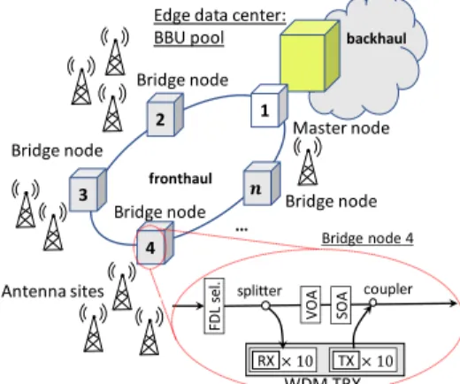
Fig. 1. N-GREEN network architecture (example of the application in the fronthaul)
TX RX Edge data center: BBU pool 1 2 3 4 Master node Bridge node Bridge node Bridge node Bridge node backhaul fronthaul Antenna sites … FD L se l. VO A SO A Bridge node 4 splitter coupler WDM TRX
II. N-GREEN NETWORK ARCHITECTURE
An example of the GREEN ring in the fronthaul and N-GREEN’s node architecture are illustrated in Fig. 1. Network is composed of 𝑛 nodes, one of which is the master node, having a role of hub and interconnecting the ring with the edge cloud. The other nodes are called the “bridge nodes”.
The N-GREEN node is composed of: a) splitters and couplers for the traffic reception/extraction via a set of WDM-TRX transponders operating at 100 Gbit/s (a single WDM-TRX operates physically with 10 single-wavelength receivers, RX, and 10 single-wavelength transmitters, TX; each RX and TX operate at 10 Gbit/s); b) variable optical attenuator (VOA) and semiconductor optical amplifier (SOA) for WDM slot blocking/bypassing and c) Fiber Delay Line (FDL) selection box, for adjusting the propagation time of the transit traffic to enable the processing of the control channel [2].
N-GREEN ring operates on a time slot basis (with time slot duration of 𝑇𝑆=1 µs). The time slots carry the “WDM slots”
which encapsulate and transport the client data simultaneously over 10 wavelengths. Note that the privileged solution for N-GREEN consists in using the WDM-TRX transponders (case called: “CONF. 1”), but to validate the techno-economic interest of N-GREEN, we also consider the case “CONF. 2” where the TRX transponders at 10 Gbit/s are used (1 TRX is composed of 1 wavelength RX and of 1 single-wavelength TX). The inserted WDM slots are separated by a guard time of 𝑇𝐺=50 ns. Regarding the control plane, the
network uses a dedicated wavelength channel for the node and network synchronization and for the transport of the control information, that is processed at each network node. The master node is connected to the SDN controller.
For statistical scheduling, WDM slot switching has been already demonstrated as highly cost efficient when compared to an electronic Ethernet technology or to a single channel approach [2]. Indeed, WDM slots allow to reduce the costs of the active components, either immediately for the optical gates that can serve for the entire ring bandwidth, either by benefiting from the savings resulting from the integrations of WDM-TRX transponders. Furthermore, N-GREEN network offers the same functionalities as Ethernet (through a processing of all the bus), while being in line with the recent Datacom technology evolution (towards WDM-TRX).
III. ZERO-JITTER AND DETERMINISTIC LATENCY SCHEDULING FOR N-GREENXHAUL
The scheduling of CPRI (or isochronous) traffic in N-GREEN consists in: a) aggregating different flows over the same transmission resource (wavelength or waveband) so that the resource use is maximized; b) properly positioning the CPRI packets within subsequent time slots to avoid any jitter and latency due to the packet insertion process and c) including the perturbation caused by the guard time in the jitter guarantees.
To address the scheduling problem, we first note that the positions of the scheduled subsequent CPRI packets in the N-GREEN time slots will vary from slot to slot, since the period
of the CPRI flow is not necessarily the same as the time slot duration 𝑇𝑆. This means that the transmission resource allocated
to the transport of CPRI flows needs to be “continuous”. The continuity can be assured either by allocating a physical channel to this transport (as seen so far) or by allocating a virtual channel to it (in CONF. 1 only). For instance, to ensure a 10 Gbit/s transport, we could either allocate a wavelength of 10 Gbit/s to it, or use a periodic “temporal slice” of sufficient capacity, e.g. we could use a 100 Gbit/s WDM TRX during 1/10 of the time. For a physical channel, the jitter introduced by the guard time 𝑇𝐺 (and limited to the value of 𝑇𝐺), in a general case,
is experienced when inserting the CPRI traffic into the optical medium. For a virtual channel, the guard time does not impact the scheduling (as it is not perceived during the emission by the source), and scheduling with zero-jitter is then achieved.
The scheduling that we propose is based on the optimal solution in form of ILP and on the greedy algorithm, defined over a scheduling cycle of size 𝑆, and minimizing the network cost (equal to the cost of network’s transponders and channels, transponders being the most expensive components). To precisely account for the CPRI packet position within a time slot, we introduce a notion of “subslot”, i.e. we suppose that each time slot is composed of exactly 𝐿 equally sized “subslots” (𝐿 is a given parameter). Let us suppose that 𝑆=𝑚 ∙ 𝐿, where 𝑚 is the number of time slots after which the scheduling is repeated cyclically by all network nodes. Next, for CPRI flow 𝑑, exchanged between nodes 𝑖 and 𝑗, we define the parameters: 𝛼(𝑖,𝑗)𝑑 - the number of subsequent subslots corresponding to a
transmission duration of a single CPRI packet and 𝛽(𝑖,𝑗)𝑑 – the
number ofsubsequent subslots between the consecutive CPRI packets (both calculated from 𝐿), and 𝐹(𝑖,𝑗)𝑑 – the number of
times the CPRI packets have to be scheduled in a single scheduler cycle 𝑆 (calculated from 𝑆). To get 𝑆, we define it as the least common multiple of numbers 𝛼(𝑖𝑑11,𝑗1)+ 𝛽
(𝑖1,𝑗1) 𝑑1 , 𝛼
(𝑖2,𝑗2)
𝑑2 +
𝛽(𝑖𝑑22,𝑗2), …, 𝐿. Finally, the value of 𝑆 allows us to find 𝑚.
As a theoretical contribution, we formulate a theorem on the scheduling of isochronous flows, that we have confirmed by the simulations. The theorem can be easily proven by contradiction and shows that the isochronous flows with periods that are not the multiples of the same base period cannot be scheduled on the same channel.
Theorem. Let 𝑃(𝑖,𝑗)𝑑 = 𝛼
(𝑖,𝑗)𝑑 + 𝛽(𝑖,𝑗)𝑑 , for all isochronous
flows defined in the scheduling problem. Then, if numbers 𝑃(𝑖𝑑11,𝑗1), 𝑃
(𝑖2,𝑗2)
𝑑2 , …, are mutually prime, the isochronous flows
cannot be scheduled on the same channel.
Note that the previous scheduling can be used also for CoE (CPRI over Ethernet) traffic. In the following, the scheduling is realized by two mathematical models: 1) as an optimal ILP program, and 2) as a scalable greedy algorithm.
IV. ILP MODEL FOR THE COST OPTIMIZED SCHEDULING
This section introduces the ILP model for calculating the slot allocation according to the previous scheduling mechanism. The resulting scheduling is cost optimized, and has the minimum cost of channel interfaces and channels, needed to
support all the traffic flows in the network. We define channel interface either as a transponder (for physical channels) or as a duration of a single temporal slice of the transponder (for virtual channel). For instance, in CONF. 1 for virtual channels, the cost of channel interface is the same as the cost of a single virtual channel, and is lower than the cost of WDM-TRX. In CONF. 1 for waveband channels and in CONF. 2, the cost of channel interface is the same as WDM-TRX and TRX cost, respectively. The input parameter to the ILP model is also the traffic matrix, defining the number of slots needed for each traffic flow. The output of the ILP model is the scheduling algorithm that shall be applied by each network node, and the network configuration, expressed in the number of the required channel interfaces and channels at each node and in the network. The full list of the input parameters for the ILP model is provided in Tab. I. For instance, the scheduling cycle size and the cost parameters are defined in this table.
Next, in Tab. II we can see all the output variables that are used for the integer linear program. Some variables are not included in Tab. II, since they are auxiliary.
Tab. III provides the list of the constraints that build the ILP model. Eq. (1) is the objective function. This function minimizes the overall cost of the N-GREEN ring, i.e. the cost of the channel interfaces and channels required in the ring. Equation (2) is the traffic-load constraint, ensuring that right amount of ring capacity is allocated to each isochronous traffic flow. Constraint (3) ensures the periodic slot allocation for the isochronous traffic demands. The constraint (4) implements the logical “IF-THEN-ELSE” condition (connecting the variables
𝑝𝑞(𝑖,𝑗),𝑑,𝑠 and𝐵𝑞(𝑖,𝑗),𝑑,𝑠 ), so it uses the auxiliary variables and
constants. Each slot can be allocated only once, per each link and channel, which is ensured by constraint (5). Constraint (6) ensures that sufficient number of transmitters and receivers are allocated at each network node.
TABLE I. INPUT PARAMETERS
Input
Parameters Definition
𝐺(𝑉, 𝐸) A directed graph representing the unidirectional N-GREEN ring, where 𝑉 is the set of nodes, 𝐸 is the set of (unidirectional) links; (|𝑉| = 𝑛 in Fig. 1); 𝑄 Set of channels (wavelengths/wavebands or virtual
channels);
𝑆 Size of the scheduling cycle (in number of subslots); 𝜋(𝑖,𝑗) Set of the links in the ring belonging to the routing
path between the nodes 𝑖 and 𝑗; 𝐷(𝑖,𝑗) Set of CPRI (isochronous) traffic demands 𝑑
between nodes 𝑖 and 𝑗 (𝐷𝑚𝑎𝑥 – the maximum
number of demands between any source-destination pair (𝑖, 𝑗));
𝛼(𝑖,𝑗)𝑑 The number of subsequent slots corresponding to a
transmission duration of a single CPRI packet for the demand 𝑑 between source-destination pair (𝑖, 𝑗); 𝛽(𝑖,𝑗)𝑑 The number of subsequent slots between the
consecutive CPRI packets for the demand 𝑑 between source-destination pair (𝑖, 𝑗); 𝐹(𝑖,𝑗)𝑑 The number of times the CPRI packets (for the
demand 𝑑 between source-destination pair (𝑖, 𝑗)) are to be scheduled in a single scheduler cycle 𝑆 ;
Input
Parameters Definition
𝐶𝑡 Cost of channel interfaces;
𝐶𝑞 Cost of a wavelength (CONF. 2), of a waveband or
of a virtual channel (CONF. 1); 𝑀1 , 𝑀2 Large constants.
TABLE II. OUTPUT VARIABLES
Output
Variables Definition
𝐵𝑞(𝑖,𝑗),𝑑,𝑠 , 𝑝𝑞(𝑖,𝑗),𝑑,𝑠
Binaries, equal to if the demand 𝑑 between (𝑖, 𝑗) is routed over channel 𝑞 starting from/by using (respectively) the subslot 𝑠, and equal to otherwise; 𝑡𝑞𝑖, 𝑟𝑞𝑖, 𝑢𝑞𝑖 Binaries, equal to if transmitter, receiver, channel
interface (respectively) at channel 𝑞 is used at node 𝑖 for the transport of traffic, and eq. to otherwise; 𝑦𝑞 Binary, equal to if channel 𝑞 is used in the ring for
the transport of traffic, and equal to otherwise.
Finally, the constraint (7) ensures the allocation of the correct number of channel interfaces at each node and channels in the network.
TABLE III. ILPFORMULATION
No. Constraint Definition
( ) 𝑀𝑖𝑛(∑𝑖∈𝑉∑𝑄𝑞=1𝐶𝑡𝑢𝑞𝑖+ ∑𝑄𝑞=1𝐶𝑞𝑦𝑞 ) (2) ∑𝑞=1𝑄 ∑𝑠=1𝑆 𝐵𝑞(𝑖,𝑗),𝑑,𝑠= 𝐹(𝑖,𝑗)𝑑 , ∀(𝑖, 𝑗)∈ 𝑉2, ∀𝑑 ∈ 𝐷(𝑖,𝑗) (3) 𝐵 𝑞(𝑖,𝑗),𝑑,𝑠1=𝐵𝑞(𝑖,𝑗),𝑑,𝑠2, ∀𝑞 ∈ 𝑄, ∀(𝑖, 𝑗) ∈ 𝑉2, ∀𝑑 ∈ 𝐷(𝑖,𝑗), (∀𝑠1, 𝑠2) ( ≤ 𝑠1, 𝑠2≤ 𝑆 ∧ 𝑠2≡ (𝑠1+ 𝑘 ∙ (𝛼(𝑖,𝑗)𝑑 + 𝛽(𝑖,𝑗)𝑑 ))𝑚𝑜𝑑 𝑆 ) (∀𝑘, 𝐹(𝑖,𝑗)𝑑 > 𝑘 ≥ ) (4) ≤ 𝑝 𝑞(𝑖,𝑗),𝑑,𝑠2− 𝐵𝑞(𝑖,𝑗),𝑑,𝑠1+ 𝑀1∙ 𝑧𝑞(𝑖,𝑗),𝑑,𝑠1, 𝐵𝑞(𝑖,𝑗),𝑑,𝑠1≤ + 𝑀2∙ ( − 𝑧𝑞(𝑖,𝑗),𝑑,𝑠1), ∀𝑞 ∈ 𝑄, ∀(𝑖, 𝑗) ∈ 𝑉2, ∀𝑑 ∈ 𝐷(𝑖,𝑗), (∀𝑠1, 𝑠2) (𝑠 ≤ 𝑠1, 𝑠2≤ 𝑆 ∧ 2≡ (𝑠1+ 𝑘)𝑚𝑜𝑑 𝑆 ) (∀𝑘, 𝛼(𝑖,𝑗) 𝑑 > 𝑘 ≥ ) (5) ∑𝑑∈𝐷(𝑖,𝑗)∑(𝑖,𝑗):𝑙∈𝜋(𝑖,𝑗)𝑝𝑞(𝑖,𝑗),𝑑,𝑠≤ , ∀𝑞 ∈ 𝑄, ∀𝑠 ∈ 𝑆 , ∀𝑙 ∈ 𝐸 (6) ∑ ∑𝑑: 𝑖=𝑠𝑜𝑢𝑟𝑐𝑒(𝑑),∑𝑆𝑠=1𝑝𝑞(𝑖,𝑗),𝑑,𝑠 𝑑∈𝐷(𝑖,𝑗) 𝑗∈𝑉:𝑙∈𝜋(𝑖,𝑗) ≤ 𝑆 ∙ 𝑡𝑞 𝑖,𝑙, ∀𝑖 ∈ 𝑉, ∀𝑞 ∈ 𝑄, ∀𝑙 ∈ 𝐸; ∑𝑙∈𝐸𝑡𝑞𝑖,𝑙≤ |𝐸|𝑡𝑞𝑖, ∑ ∑𝑑: 𝑖=𝑑𝑒𝑠𝑡(𝑑),∑𝑆𝑠=1𝑝𝑞(𝑗,𝑖),𝑑,𝑠 𝑑∈𝐷(𝑖,𝑗) 𝑗∈𝑉 ≤ 𝑆 ∙ 𝑟𝑞𝑖, ∀𝑖 ∈ 𝑉, ∀𝑞 ∈ 𝑄 (7) 𝑡𝑞𝑖+ 𝑟𝑞𝑖≤ 2 ∙ 𝑢𝑞𝑖, ∀𝑖 ∈ 𝑉, ∀𝑞 ∈ 𝑄; ∑𝑖∈𝑉𝑡𝑞𝑖,𝑙≤ ,∀𝑞 ∈ 𝑄, ∀𝑙 ∈ 𝐸; ∑𝑖∈𝑉𝑢𝑞𝑖 ≤ |𝑉| ∙ 𝑦𝑞, ∀𝑞 ∈ 𝑄
V. HEURISTIC SOLUTION FOR THE SCALABLE SCHEDULING IN
N-GREENXHAUL
The cost-optimized scheduling described in the previous section consumes important computing time when the ILP program is implemented, but no formal proof about its computational complexity is available yet. For the real network implementation of the scheduling, it would be excellent to have a faster algorithm, that is adapted to a fast execution at the SDN controller. With goal of addressing this problem, in the current section we propose a greedy algorithm, that addresses the same scheduling problem that is already introduced, and that has the same input parameters and output variables as the ILP (with exception of the constants 𝑀1 , 𝑀2).
The name of the proposed algorithm is “Greedy Source Cost Minimization” (GSCM), and its pseudocode is provided in Tab. IV. The algorithm name comes from its intention to ensure the minimization of the number of channel interfaces (transponders) and consequently the cost of each source in the network. The “group of flows” in the algorithm is defined as a set of flows generated by the same source. In steps 2-6 of the algorithm, the group of flows are taken in the decreasing order and routed according to the first-fit channel assignment method. Next, in steps 7-13, the algorithm applies the same procedure, but this time for each network node separately, which has shown to have cost saving advantages for more centralized traffic matrices (like “hub and spoke” scheme, as introduced in the following section). Finally, in the steps 14-16, the algorithm GSCM chooses its best solution.
TABLE IV. PSEUDOCODE OF THE ALGORITHM:GREEDY SOURCE COST
MINIMIZATION (GSCM)
1: Input: the same as for the ILP model (with exception of the constants 𝑴𝟏 , 𝑴𝟐 which are not needed)
2: Sort the groups of flows in order of decreasing traffic rate 3: for each group of flows taken in this order do
4: First-fit channel assignment of the group of flows, by always assigning first the resources (channel interfaces and channels) to the highest flow in the group of flows
5: end for
6: Compute the overall network cost 𝑪𝑻𝑶𝑻
7: for each network node A
8: Sort the groups of flows exchanged between nodes A and its destinations in order of decreasing traffic rate
9: for each group of flows taken in this order do
10: First-fit channel assignment of the group of flows, by always assigning first the resources to the highest flow in the group of flows 11: end for
12: end for
13: Compute the new overall network cost 𝑪𝑻𝑶𝑻′ 14: if (𝑪𝑻𝑶𝑻′ < 𝑪𝑻𝑶𝑻 ) then
15: Accept the new design 16: end
VI. NUMERICAL RESULTS
In this section, we report the simulation results obtained by using both the ILP and GSCM tools, to estimate the cost and energy consumption of the N-GREEN network.
Regarding the traffic matrix, CPRI or isochronous traffic flows, for the packet size of 1250 bytes and 10 Gbit/s channel capacity, are chosen from the sets 𝐴1= {2.5, 5, } Gbit/s [1]
and 𝐴2= { .67, 3.33, 6.67} Gbit/s, that have different basic
periods. Under these assumptions, for different simulations, we consider one of the following four traffic scenarios:
a) Scenario 1: The traffic profile is “hub-and-spoke” (more precisely we suppose that each bridge node communicates with the master node, and vice versa, and that the amount of traffic exchanged in both directions in this communication is the same). Next, 𝑚 = 4, 𝐿 = , 𝑆 = 4. Each bridge node sends the traffic from set 𝐴1 (to the master node), resulting in a uniform
and symmetric traffic. b) Scenario 2: The traffic profile is hub-and-spoke, with 𝑚 = 4, 𝐿 = 3, 𝑆 = 2. Each bridge nodes sends three randomly chosen flows from the set 𝐴1∪ 𝐴2.
c) Scenario 3: The source, destination and flow type are all randomly distributed. Each bridge nodes sends three randomly
chosen flows from the set 𝐴1∪ 𝐴2. We suppose that 𝑚 =
4, 𝐿 = 3, 𝑆 = 2. d) Scenario 4: The traffic profile is hub-and-spoke, with 𝑚 = 4, 𝐿 = 3, 𝑆 = 2. Each bridge nodes sends three randomly chosen flows from the set 𝐴1∪ 𝐴2, for different
ring size 𝑛.
A. The results obtained by using the ILP model
We implement the ILP model in IBM CPLEX software (for 𝑛 = 6, 𝐶𝑡= [a.u.] for 10 Gbit/s channel interfaces (CONF. 1
or 2), 𝐶𝑞 << 𝐶𝑡, i.e. 𝐶𝑞= . [a.u.]) and report the optimal
simulation results in Figs. 2-5, for Scenarios 1 and 2. In all the simulations, the cost 𝐶𝑞 corresponds either to the cost of a
wavelength or of a virtual channel. Indeed, for such channels, the value of cost 𝐶𝑞 is the same, since the equivalent capacity
of a wavelength or of a virtual channel is the same and equal to 10 Gbit/s. Finally, in all scenarios in this work, the simulations are run for the gradually increasing traffic, by adding to the traffic matrix in each step the traffic contribution (the sent and received traffic) for the next bridge node in the network, until all the bridge nodes have been accounted for.
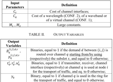
Fig. 2 shows the number of channel interfaces and channels in the network, for Scenarios 1 and 2. The number of channel interfaces is higher than number of channels for both scenarios, while Scenario 2 is more expensive. For Scenario 2, the traffic is random, resulting in a non-linear increase of the number of channel interfaces and channels. The channel occupancy (of physical channels, i.e. wavelengths or virtual channels) in N-GREEN is illustrated in Fig. 3. The channel occupancy reaches high values (≈90%) meaning that the N-GREEN network with the proposed scheduler is highly efficient in the resource use.
Fig. 2. Number of channel interfaces and channels (for Scenarios 1 and 2)
The number of transponders in Scenario 2 for an equivalent Ethernet ring (with TRXs at 10 Gbit/s) and for different variants of N-GREEN are compared in Fig. 4. For N-GREEN we consider two cases: 1) CONF. 2, i.e. nodes equipped with several TRX at 10 Gbit/s (with physical channels, i.e. with single wavelength per TRX) and 2) CONF. 1, i.e. nodes equipped with several WDM-TRX at 100 Gbit/s (supporting 10 virtual channels at 10 Gbit/s). Fig. 4 shows the significant savings when the WDM TRX are used (up to 9 times).
Next, the transponder cost is compared in Fig. 5, for the following assumptions:
1) Since burst mode TRX operation at 10 Gbit/s results in a small additional logic [4], the cost of TRX in Ethernet and N-GREEN (CONF. 2, physical channels at 10 Gbit/s) is approximately the same and equal to 𝐶𝑡= [a.u.];
Fig. 4. Number of transponders for Scenario 2. Results show potential savings of N-GREEN vs Ethernet (up to 9 times) in number of transponders.
Fig. 5. Transponder cost for Scenario 2. Results show potential savings of N-GREEN vs Ethernet in the cost of transponders (savings up to 33% when WDM-TRX are used).
TABLE V. COMPARISON BETWEEN N-GREEN AND ETHERNET FRONTHAUL
2) The cost of WDM-TRX (CONF. 1, virtual channels) is supposed to be 𝛿 ∙ 𝐶𝑡 (where parameter 𝛿 ∈[1,10]).
Fig. 5 shows important savings of N-GREEN in transponder cost w.r.t. Ethernet for physical channels. For virtual channels, the savings up to 33% are achieved for 𝛿 ≤ 6, which seems achievable since the cost of a single 10 Gbit/s TRX is ≈250 $ [5] and the cost of WDM-TRX is expected to be ≤6∙250 =1500$ thanks to the laser integration design of these devices. Finally, Tab. V compares the sources of jitter and latency in N-GREEN and Ethernet. While variable in Ethernet [1], latency is fixed in N-GREEN in transit and at the insertion, and the jitter is different than zero (and limited to 𝑇𝐺) only for the physical
channel scheduling in N-GREEN. When channel is virtual the jitter is equal to zero.
B. The validation of the GSCM algorithm
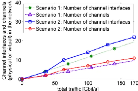
To validate the GSCM algorithm, we compare the optimal solution (OPT) calculated by the ILP model, and the solution found by GSCM algorithm, in a randomly generated Scenario 3 (to test the GSCM performance in the most general case). The results are presented in Fig. 6. The simulations are performed for different value of the cost ratio between the cost of channel interface and the cost of channel. The following cost assumptions are considered: 1) 𝐶𝑡= , 𝐶𝑞= . , 2) 𝐶𝑡=
, 𝐶𝑞= , and 3) 𝐶𝑡= . , 𝐶𝑞= . The results suggest that
GSCM obtains excellent performances on the selected random traffic scenario, and its results are very close to the optimal solution. The highest discrepancy from the optimal solution was less than 5%, and this performance was not affected by the change of the cost ratio of channel interface and channels.
We have also compared the solution found by the GSCM and ILP model on the hub-and-spoke Scenario 2, that is centralized, and 0% error of the GSCM (w.r.t. the optimal solution) has been observed. Such good results of GSCM algorithm can be explained by the fact that the channels for transport of the isochronous traffic need to be allocated per source, to preserve the “continuity” of the channel, as previously discussed, which allows to eliminate or to limit the jitter. Because of this, different sources are not allowed to use the same channel over the same links, which allows good results to the heuristics based on the greedy approach in optimizing the source cost.
C. The results obtained by using the GSCM algorithm The proposed GSCM is scalable. Indeed, its complexity is limited to 𝑂(𝑛3𝐷
𝑚𝑎𝑥), i.e. this is a polynomial time algorithm.
In the current section, we exploit the algorithm GSCM to compare the cost and energy consumption of N-GREEN and Ethernet for a greater and a realistic size of the N-GREEN network of up to 10 nodes.
The simulations are performed for Scenario 4, and for different rings sizes. The transponder cost comparison between N-GREEN and Ethernet is presented in Fig. 7. From the figure, we can see that the savings of N-GREEN w.r.t. Ethernet increase with the increase of ring size. When the network is sufficiently loaded, even if the ring size is not large (𝑛 = 6), N-GREEN network costs much less than Ethernet, measured in transponder cost. If the integration technology used for production of the WDM-TRX transponders enables the cost
N-GREEN Ethernet
Jitter at insertion 0 or ≤ 𝑇𝐺 (for
physical channels) ~ µ𝑠 [1]
Jitter in transit 0 Depends on traffic
load and network size
Latency at insertion & transit
reduction of these devices of 𝛿 ≤ 3, the potential savings of costs go to more than 6 times, obtained for 𝑛 = . For 𝛿 ≤ 6, the savings are more than 3 times (result not shown in the figure), etc.
Fig. 7. Transponder cost for different ring sizes in Scenario 4 (results of GSCM algorithm). Results show high potential savings of N-GREEN vs Ethernet in the cost of transponders (more than 3 times when WDM-TRX are used)
Fig. 8. Power consumption of N-GREEN vs Ethernet in Scenario 4 (results of GSCM algorithm). Results show high potential savings of NGREEN vs Ethernet (up to 10 times) in power consumption.
Fig. 8 shows the power consumption performance of N-GREEN and Ethernet, in Scenario 4. For Ethernet, we suppose the consumption of each SFP+ 10 Gbit/s TRX to be 1.5 W [6] and the switching fabric consumption to be ≈5W/port (calculated from [7]). For N-GREEN, the consumption of SOA is 1.5W, while 5W is the estimated consumption of the electronic part of the node. The consumption of WDM-TRX is 5W [8]. From Fig. 8 we can see that N-GREEN achieves significant savings (up to 10 times) in the power consumption, when compared with Ethernet.
VII. CONCLUSION
A cost optimized and deterministic scheduler for the N-GREEN WSADM technology, supporting the time-sensitive CPRI traffic with zero jitter has been proposed. Then, an Integer Linear Program and a highly performant heuristic have been provided as tools enabling to calculate this scheduling. The benchmarking studies have been performed and have shown that significant cost and energy consumption reductions could be obtained when compared to a same capacity state-of-the-art Ethernet technology. The WDM technology proposed in the N-GREEN project is positioning as a highly competitive solution for a future generation of Xhaul networks.
ACKNOWLEDGMENT
We thank François Taburet for the insightful exchanges about the topic. We thank the French National Agency of Research (ANR) for partial funding of the N-GREEN project.
REFERENCES
[1] D. Chitimalla et al., "5G fronthaul-latency and jitter studies of CPRI over ethernet," in IEEE/OSA JOCN, Feb. 2017.
[2] D. Chiaroni and B. Uscumlic, "Potential of WDM Packets”, invited paper, ONDM 2017, Budapest, Hungary, 2017.
[3] A. Triki, A. Gravey, P. Gravey, M. Morvan, “Long-Term CAPEX Evolution for Slotted Optical Packet Switching in a Metropolitan Network”. ONDM 2017, Budapest, Hungary, 2017.
[4] Xilinx All Programmable, XAPP1252 (v1.1) November 17, 2016, “Burst-Mode Clock Data Recovery with GTH and GTY Transceivers”, Author: Edward Lee and Caleb Leung,
https://www.xilinx.com/support/documentation/application_notes/xapp1 252-burst-clk-data-recovery.pdf, accessed on Oct. 29, 2017.
[5] Cost of 10G DWDM SFP+ Transceivers (found at https://www.cozlink.com/), https://www.cozlink.com/10g-dwdm-sfp-transceivers-c322-323-zh381, accessed on Oct. 29, 2017.
[6] Finisar, Product Specification, 10Gb/s, 40km Single Mode, Multi-Rate SFP+ Transceiver, FTLX1672D3BTL,
https://www.finisar.com/sites/default/files/downloads/finisar_ftlx1672d3 btl_10gbase-er_40km_sfp_optical_transceiver_product_specb1.pdf, accessed on Oct. 29, 2017.
[7] Cisco Catalyst 2960-S Series Switches Data Sheet,
https://www.cisco.com/c/en/us/products/collateral/switches/catalyst-2960-s-series-switches/data_sheet_c78-726680.html, accessed on Oct. 29, 2017.
[8] Cisco CPAK 100GBASE Modules Data Sheet,
https://www.cisco.com/c/en/us/products/collateral/interfaces-modules/transceiver-modules/data_sheet_c78-728110.html, accessed on Oct. 29, 2017