Uncertainty Estimation in Indirect Calibration of Five-Axis Machine Tools

(1)

UNIVERSITÉ DE MONTRÉAL

UNCERTAINTY ESTIMATION IN INDIRECT CALIBRATION OF FIVE-AXIS MACHINE TOOLS

ANNA LOS

DÉPARTEMENT DE GÉNIE MÉCANIQUE ÉCOLE POLYTECHNIQUE DE MONTRÉAL

THÈSE PRÉSENTÉE EN VUE DE L’OBTENTION DU DIPLÔME DE PHILOSOPHIAE DOCTOR

(GÉNIE MÉCANIQUE) MAI 2017

(2)

ÉCOLE POLYTECHNIQUE DE MONTRÉAL

Cette thèse intitulée :

UNCERTAINTY ESTIMATION IN INDIRECT CALIBRATION OF FIVE-AXIS MACHINE TOOLS

présentée par : LOS Anna

en vue de l’obtention du diplôme de : Philosophiae Doctor a été dûment acceptée par le jury d’examen constitué de :

M. BARON Luc, Ph. D., président

M. MAYER René, Ph. D., membre et directeur de recherche M. KHAMENEIFAR Farbod, Ph. D., membre

(3)

DEDICATION

“Normal people... believe that

if it ain't broke, don't fix it.

Engineers believe that

if it ain't broke, it doesn't have enough features yet.” Scott Adams

(4)

ACKNOWLEDGEMENTS

Firstly, I would like to express my deepest gratitude to my advisor Prof. René Mayer for the continuous support of my Ph. D. study and related research, for his patience, motivation, and immense knowledge.

My sincere thanks goes to my thesis committee: Prof. Andreas Archenti, Prof. Luc Baron, Prof. Farbod Khameneifar and Prof. Guillaume-Alexandre Bilodeau, for their time, insightful comments and their acceptance to join the jury.

I would like to thank Guy Gironne and Vincent Mayer, CNC technicians, and François Ménard, CMM technician, for their assistance at Virtual Manufacturing Research Laboratory (LRFV) in Polytechnique Montréal.

I am also grateful to the NSERC Canadian Network for Research and Innovation in Machining Technology (CANRIMT) for funding this PhD research.

I would like to thank my fellow doctoral students for their feedback, cooperation and of course friendship: Tibet Erkan, Najma Alami-Mchichi, Maryam Aramesh, Michal Rak, Mehrdad Givi and Elie Bitar-Nehme.

I would like to express my gratitude to my family and friends, with special thanks to Anna and Marek Balazinski, for always being there for me.

Last but not the least, I would like to thank my friend and love Xavier Rimpault for his endless support and always believing in me.

(5)

RÉSUMÉ

La calibration de machine-outil est un processus critique qui vise à maintenir la précision de la machine et, par conséquent, la qualité d’usinage aux niveaux requis. Différentes méthodes de mesures et instruments sont utilisés pour acquérir l’information de la géométrie de la machine. Les résultats de calibration sont exploités pour corriger et compenser les erreurs de la machine. Ainsi, ils devraient être évalués par rapport à leur incertitude.

Dans cette thèse, la méthode de calibration de l’artefact de l’échelle et des billes de référence (SAMBA) est estimée au travers de son incertitude. L’exécution de SAMBA nécessite de palper l’artefact non-calibré sous différentes indexations des axes de rotation de la machine et la barre d’échelle au moins une fois. Le calcul du centre des billes, introduit au sein du modèle cinématique de la machine, permet d’estimer les paramètres d’erreur géométrique de la machine (grandeur de sortie). La méthode proposée de l’estimation d’incertitude prend en compte que la calibration analysée a un modèle à entrées multiples et sorties multiples ainsi qu’une solution itérative. Ainsi, le Guide pour l'Expression de l'incertitude de mesure Supplément 2 (GUM S2) est suivi.

L’incertitude du palpage (grandeur d’entrée) est évaluée au travers de mesures répétées, ce qui permet de calculer les incertitudes types, la covariance et la fonction de densité de probabilité (PDF). Cette incertitude inclue la machine (mesurandes), le palpeur et les incertitudes de l’artefact. De sorte à inclure la performance de la machine dans le bilan d’incertitude, les mesures répétées sont effectuées avec différentes conditions préalables de calibration (avec et sans cycle de réchauffement) sur 24 heures. À l’étape suivante de la recherche, les variations à court et moyen terme dans la mesurande sont analysées en exécutant des mesures répétées de SAMBA sur cinq jours. L’incertitude d’entrée est propagée aux paramètres géométriques de la machine grâce à la méthode de Monte Carlo (MCM). L’incertitude de sortie est estimée avec la structure d’incertitude complète (incertitudes types et covariance) et avec les incertitudes estimées étendues, et avec le facteur d’élargissement approprié pour un modèle à multiples sorties. Le cadre de travail général sur l’incertitude - une alternative au long processus de la MCM - est appliqué en utilisant le Jacobien et validé avec la MCM.

Les recherches menées montrent que les résultats de calibration dépendent de la performance de la machine et de ses variations se produisant dans le temps et à cause de différentes conditions environnementales. Cet impact est montré par les différents types des incertitudes estimées. De

(6)

cette façon, le comportement de la machine est inclus dans le résultat de calibration, qui à lui seul, reflète l’état de la machine seulement au moment de la calibration.

(7)

ABSTRACT

Machine tool calibration is a critical process to maintain the machine precision and, therefore, the machining quality at the required levels. Different measuring methods and devices are used to acquire information about machine geometry. The calibration results are used to correct and compensate the machine errors. Thus, they should be evaluated through their uncertainty.

In this thesis, the scale and master balls artefact (SAMBA) calibration method is evaluated through its uncertainty. Conducting SAMBA requires probing the uncalibrated artefact in different machine rotary axes indexations and the scale bar at least one. The calculated balls centers introduced in the machine kinematic model allow estimating the machine geometric error parameters (output quantity). The proposed uncertainty estimation method takes into account that the analyzed calibration has a multi-input multi-output model and an iterative solution, which prevents from applying traditional uncertainty estimation techniques. Thus, the Guide to the Expression of Uncertainty in Measurement Supplement 2 (GUM S2) is followed.

The probing (input quantity) uncertainty is estimated through the repeated measurement, which allows calculating its standard uncertainties, covariance and probability density function (PDF). This uncertainty includes the machine (measurand), probe and the artefact uncertainties. In order to include the machine performance in the uncertainty budget, the repeated measurements are conducted with different calibration pre-conditions (with and without the warm-up cycle) over 24 hours. In the next stage of research, the short- and medium-term variations in measurand are analyzed by conducting SAMBA repeated measurement over five days. The input uncertainty is propagated on the machine geometric error parameters through the Monte Carlo method (MCM). The output uncertainty is estimated with its full uncertainty structure (standard uncertainties and covariance) and expanded uncertainties estimated with the appropriate, for a multi-output model, coverage factor. The GUM uncertainty framework (GUF) - alternative to the time-consuming MCM - is applied using the numerical Jacobian and validated with MCM.

The conducted research depicts that the calibration results depend on the machine performance and its variations occurring in time and due to the different environmental conditions. This impact is demonstrated by the different types of uncertainties estimated. That way the machine “behavior” is included in the calibration result, which alone reflects the machine state only at the moment of calibration.

(8)

LIST OF TABLES

Table 2.1: Estimated machine geometric error parameters (Mayer, 2012) ... 15

Table 4.1: Identified machine geometric error parameters ... 35

Table 5.1: Identified machine geometric error parameters ... 52

Table 5.2: Correlation coefficients rall between the coordinates of the three master balls... 55

Table 5.3: Correlation coefficients rpooled between the coordinates of the three master balls ... 56

Table 6.1: Identified machine geometric parameters [3] ... 70

Table 7.1: GUF and MCM machine geometric errors results comparison ... 76

Table 7.2: GUF and MCM machine geometric errors results uncertainties comparison ... 76

Table 7.3: GUF and MCM coverage factors and correlation matrix maximum eigenvalue results comparison ... 77

Table 7.4: Output quantity correlations for GUF results ... 77

Table 7.5: Output quantity correlations for MCM results obtained for M = 103 ... 78

(13)

LIST OF FIGURES

Figure 2.1: Examples of different topology of multi-axis machines (Schwenke et al., 2008) ... 4 Figure 2.2: Machine tool accuracy over the past century (Byrne, Dornfeld, & Denkena, 2003) .... 5 Figure 2.3: Ishikawa diagram with machine error sources (Jamshidi, Maropoulos, Chappell, &

Cave, 2015) based on (Lamikiz et al., 2009) ... 6 Figure 2.4: Link and location errors of linear and rotation axes (Schwenke et al., 2008) ... 8 Figure 2.5: Y-axis position error measurement using laser interferometry (Schwenke et al., 2008) ... 9 Figure 2.6: Error measurement using the kinematic ball-bar (Jae Pahk et al., 1997) ... 11 Figure 2.7: left: Schematic configuration of the pseudo-3D-artefact; right: linear displacement

measurement system with four sensors(Bringmann et al., 2005) ... 11 Figure 2.8: Cap-ball measurement system (Zargarbashi & Mayer, 2009) ... 12 Figure 2.9: Artefact configuration on five-axis machine (Erkan et al., 2011) ... 13 Figure 2.10: SAMBA artefact with twenty four master balls mounted on the machine tool (Mayer,

2012) ... 14 Figure 2.11: Axis location errors of a machine tool with WCBXFZYT topology (Mayer, 2012) 14 Figure 2.12: Indigenous artefact probing on the wCAYFXZ(C1)t machine tool (Mayer et al., 2015) ... 16 Figure 3.1: Thesis organization chart ... 24 Figure 4.1: left: Five-axis CNC machine model with the topology WCBXFZY(C1)T;

W - workpiece, T - tool, F - machine foundation, B, C – rotary axes around the Y and Z axes respectively, X, Y, Z – machine linear axes, S – spindle; right: SAMBA artefact being probed using the Renishaw probe MP700 on a Mitsui Seiki HU40-T machine tool ... 28 Figure 4.2: SAMBA identification flow chart ... 29 Figure 4.3: Adaptive MCM scheme applied to the SAMBA calibration method ... 33

(14)

Figure 4.4: X-, Y- and Z- coordinates of ball 1 obtained from the repeated measurements in [b, c] = [90°, 270°] with (bottom) and without (top) the warm-up cycle ... 36 Figure 4.5: Probing results of balls 3 and 4 obtained from the repeated measurements

in [b, c] = [90°, 270°] with (right) and without (left) the warm-up cycle ... 37 Figure 4.6: Repeated SAMBA calibration results for Cold-Cold and Hot-Cold test with three

uncertainties for p = 0.95... 40 Figure 4.7: MCM results for Cold-Cold (bottom) and Hot-Cold (top) with the estimated expanded

rectangular uncertainties for p = 0.95 for EXOC vs. ECOB (left) and EAOY vs. EAOB (right) (only

1% of the results are depicted for graph clarity reasons) ... 41 Figure 5.1: SAMBA artefact being probed using the touch trigger probe on the Mitsui Seiki HU40-T machine tool with the topology WCBXbZY(C1)HU40-T; W – workpiece, HU40-T – tool, b – machine bed, B, C – rotary axes around the Y and Z axes respectively, X, Y, Z – machine linear axes, C1 – spindle ... 49 Figure 5.2: Examples (A, B, C) of X, Y and Z coordinate probing variations of master balls (left)

and uncertainty calculated for each day, using all the data and pooled by days (right) ... 53 Figure 5.3: Histograms of the p-values for the Bartlett’s test and one-way ANOVA estimated for

all the probing data ... 54 Figure 5.4: Calibration uncertainty values including short- and medium-term measurand changes

for the confidence level p = 0.95 with the p-value of the Bartlett’s test and one-way ANOVA ... 58 Figure 5.4 (continued): Calibration uncertainty values including short- and medium-term

measurand changes for the confidence level p = 0.95 with the p-value of the Bartlett’s test and one-way ANOVA ... 59 Figure 5.4 (continued): Calibration uncertainty values including short- and medium-term

measurand changes for the confidence level p = 0.95 with the p-value of the Bartlett’s test and one-way ANOVA ... 60

(15)

Figure 5.4 (continued): Calibration uncertainty values including short- and medium-term measurand changes for the confidence level p = 0.95 with the p-value of the Bartlett’s test and one-way ANOVA ... 61 Figure 5.4 (continued): Calibration uncertainty values including short- and medium-term

measurand changes for the confidence level p = 0.95 with the p-value of the Bartlett’s test and one-way ANOVA ... 62 Figure 6.1: left: SAMBA artefact probed on the machine tool for [b, c]=[0, 0]; right: five-axis

machine tool kinematic model with the topology WCBXbZYC1T; W - workpiece, T - tool, b

- machine base, B, C – rotary axes around the Y and Z axes respectively, X, Y, Z – machine linear axes, C1 – spindle ... 67

Figure 6.2: SAMBA flow chart ... 68 Figure 6.3: Uncertainty values for different numbers and configurations of SAMBA artefact for

(16)

LIST OF SYMBOLS AND ABBREVIATIONS

Abbreviations

ANOVA Analysis of variance

ASME American Society of Mechanical Engineers BIMP Bureau International des Poids et Mesures CMM Coordinate measuring machine

CNC Computer numerical control

GUM Guide to the Expression of Uncertainty in Measurement

GUM S1 Guide to the Expression of Uncertainty in Measurement Supplement 1 GUM S2 Guide to the Expression of Uncertainty in Measurement Supplement 2 GUF GUM uncertainty framework

HTM Homogeneous Transformation Matrices ISO International Organization for Standardization JCGM Joint Committee for Guides in Metrology

MC Monte Carlo

MCM Monte Carlo method

MIMO Multi-input multi-output PDF Probability density function

RUMBA Reconfigurable uncalibrated master ball artefact SAMBA Scale and master balls artefact

Symbols

B Machine rotary axis around Y

b Machine bed

(17)

C Machine rotary axis around Z

c Indexation of C-axis

C1 Machine spindle

𝑪𝒙 Sensitivity matric associated with input quantity

𝒅 Initial dimension of artefact

𝑑 Validation parameter

𝒆_𝑣 Volumetric error

EAOB Out-of-squareness of the B-axis relative to the Z-axis

ECOB Out-of-squareness of the B-axis relative to the X-axis

EXOC Distance between the B and C axes

EAOC Out-of-squareness of the C-axis relative to the B-axis

EBOC Out-of-squareness of the C-axis relative to the X-axis

EBOZ Out-of-squareness of the Z-axis relative to the X-axis

EAOY Out-of-squareness of the Y-axis relative to the Z-axis

ECOY Out-of-squareness of the Y-axis relative to the X-axis

EXOC1 X offset of the spindle relative to the B-axis

EYOC1 Y offset to the spindle relative to the C-axis

EXX Positioning linear error term of the X-axis

EYY Positioning linear error term of the Y-axis

EZZ Positioning linear error term of the Z-axis

F Machine foundation

𝑱 Jacobian matrix

𝑱+ _{Pseudoinverse Jacobian matrix}

(18)

𝑘_𝑝 Coverage factor for hyper-ellipsoidal coverage region 𝑘𝑞 Coverage factor for hyper-rectangular coverage region

𝐿 Scale bar calibrated length

𝜆_𝑚𝑎𝑥 Maximum eigenvalue of correlation matrix 𝑹_𝒚

𝜏 Machine geometric error parameter adjustment threshold 𝑀 Number of Monte Carlo simulations

𝑚 Number of output quantities 𝑁 Number of input quantities

𝑝 Coverage probability

p-valueA p-value from ANOVA

p-valueB p-value from Bartlett’s test

𝑷_{𝑏𝑎𝑙𝑙} Ball center position 𝑷_𝑡𝑖𝑝 Tool tip position

𝑹𝐴𝑂𝐶 Rotation matrix around X-axis

𝑹𝒚 Correlation matrix associated with the estimate 𝒚 of output quantity 𝒀

𝑟(𝑥_𝑖,𝑥_𝑗,) Correlation coefficient between the estimates 𝑥_𝑖 and 𝑥_𝑗

𝑟𝑎𝑙𝑙(𝑥𝑖,𝑥𝑗,) Correlation coefficient between the estimates 𝑥𝑖 and 𝑥𝑗 (obtained with all the data)

𝑟_{𝑝𝑜𝑜𝑙𝑒𝑑}(𝑥_𝑖,𝑥_𝑗,) Pooled Correlation coefficient between the estimates 𝑥_𝑖 and 𝑥_𝑗 𝒔 Standard deviation

T Tool

𝑻𝐵0

𝑋′

Homogenous transformation matrix of the nominal B-axis location relative to the actual X-axis carriage

𝑻𝑡𝑖𝑝 𝑏𝑎𝑙𝑙

(19)

𝑼𝒙 Covariance matrix associated with estimate 𝒙 of input quantity 𝑿

𝑼𝒙 pooled Pooled covariance matrix associated with estimate 𝒙 of input quantity 𝑿

𝑼𝒚 Covariance matrix associated with estimate 𝒚 of output quantity 𝒀

𝑈_𝑝 Expanded uncertainty for the coverage probability p

𝑢 Standard uncertainty

W Workpiece

X Machine linear axis

𝑿 Input quantity

𝒙 Estimate of input quantity 𝑿

𝒙_𝑅 Residual volumetric prediction error

Y Machine linear axis

𝒀 Output quantity

𝒚 Estimate of output quantity 𝒀

𝒚̃ Estimate of output quantity from Monte Carlo method results

(20)

CHAPTER 1 INTRODUCTION

“The history of machine tools is the history of the precision of machine tools.” Lamikiz et al.(Lamikiz, López de Lacalle, & Celaya, 2009) In the manufacturing area, material removal machining is a major process. Machining precision has been improving since the first machine tools were constructed and this progress continues. The ability to machine with narrower geometrical tolerances is a key component in terms of part and assembly design evolution. Increasing the quality of the final workpiece requires an even bigger increase in the machining precision. This parameter is crucial when a new machine is being designed and, even later, all along its life in service. The last few decades have brought significant changes in the machine tools performance and features. The computer numerical control (CNC), automated tool change, on-machine measurement etc. allow manufacturing a workpiece faster, with tighter tolerances and more complex design.

One of the most important parameters of a machine specification is its precision. It refers to the machine positioning accuracy (the ability to indicate the nominal value) and repeatability (the dispersion of the results when showing the same value). The resolution is also considered as an important factor since it represents the smallest position change that machine axis encoders can detect.

Evaluating and maintaining desired precision levels requires identifying the sources of machine inaccuracies. Among thermal, geometric, kinematic and dynamic errors, the geometric ones have the most significant impact on the machine positioning accuracy. Various calibration methods have been developed that allow testing and verifying those errors. Machine tool calibration gives the information about the machine geometry and, depending on the method and the applied model, it results in one (single-output) or a number of identified geometric error parameters (multi-ouput). Machine calibration is a subject of numerous research projects. Moreover, it has to be one step ahead of the machine precision progress.

1.1 Problem definition

The calibration of machine tool has to be performed frequently to ensure the machine ability to keep the required precision. The information about the machine performance obtained during the

(21)

calibration is later used, when the decision about error correction or compensation is made. Thus, the calibration results should be evaluated through their uncertainty as any other measurement result. The estimation of calibration uncertainty is a challenging task. The main uncertainty sources include the artefact or measuring device calibration uncertainty (if present), environmental conditions, and the machine itself (because its performance changes). In this case the machine is an uncertainty source and the measurand (measured quantity) itself. How to estimate the uncertainty on the quantities that are being estimated? Moreover, if an uncalibrated artefact is used in the calibration, it has no calibration uncertainty but its geometry variations may impact the results. How to include this influence in uncertainty budget? If the calibration method is non-linear and iterative, how the uncertainty can be propagated on the results? When applied method has a multi-output, should this be considered in data analysis? In this thesis the methodology and the experiments are presented to answer these questions since there is no available standard that would give full and comprehensive guidance to the highlighted issues.

1.2 Objectives

The main objective of this thesis is to develop a procedure that allows estimating the uncertainty of indirect calibration methods with an iterative solution and multi-output.

The secondary objectives include:

1) Estimating the measurement uncertainty of the uncalibrated artefact probing with full uncertainty structure;

2) Estimating the uncertainty on the calibration results that includes machine (measurand) performance;

3) Propagating the uncertainty on the calibration results using a method that is time-efficient and appropriate for multi-input multi-output iterative models;

4) Estimating the input and output uncertainty with the full uncertainty structure (standard uncertainties and covariance).

1.3 Hypotheses

(22)

1) Machine has the rigid body kinematics;

2) The applied geometric error model is optimized. The errors model is not part of the evaluation in this thesis;

3) The probing measurement has a normal distribution - the hypothesis of normal distribution is assumed and tested using statistical normality tests;

4) The repeated calibration measurement gives the estimate of its standard uncertainty, covariance and normal distribution parameters (mean and variance).

(23)

CHAPTER 2 LITERATURE REVIEW

In this chapter, the state of the art in the machine performance testing is presented. Firstly, the machine different structures are presented. Then, the main machine errors sources are listed and various calibration methods are described. The standards for testing the machine performance and for uncertainty estimation are briefly discussed. The detailed strategies and methodology of the calibration uncertainty estimation are to be described in the articles following the literature review.

2.1 Multi-axis machines

Multi-axis machines are widely used in manufacturing for various machining operations (machine tools) and measurements (coordinate measuring machines (CMMs)). CMMs traditionally have a three-axis topology with different configuration of the linear axes. Modern machine tools, except for three linear axes (X, Y, Z), have additional two rotary axes (B, C). Examples of different topologies of five-axis machines are shown in Figure 2.1.

(24)

The machine tool geometry has a kinematic structure, which includes machine components (workpiece w (or W), tool t (or T) and machine bed b (or F - foundation)) and linear (X, Y and Z) and rotary axes (B, C) (Abbaszadeh-Mir, Mayer, & Fortin, 2003; Mir, Mayer, & Fortin, 2002; Schwenke et al., 2008). Most of the machines have serial structure. It means that all the axes move independently from one another.

When the machine is about to be purchased or designed the following requirements are considered (López de Lacalle & Lamikiz, 2009): the maximum part size, workpiece main geometry (for a cylindrical shape, the lathe machine is considered in the first place), second geometry (design complexity), material removal rate and, finally, precision.

2.2 Machine performance

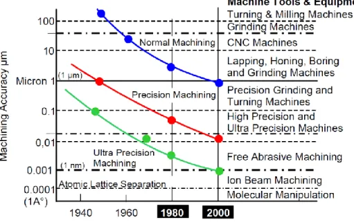
Machine precision is defined by its positioning accuracy (difference between the actual and nominal values) and repeatability (caused by the random sources expressed as the range of variations for the same position) (Lamikiz et al., 2009). The precision of the manufactured machine tool has been significantly increasing over the time. The evolution of machine tool accuracy in the previous century is presented in Figure 2.2.

Figure 2.2: Machine tool accuracy over the past century (Byrne, Dornfeld, & Denkena, 2003) The positioning accuracy of the tool and workpiece has a direct impact on the volumetric error (relative position of the workpiece to tool) and therefore, the quality of machined parts. The

(25)

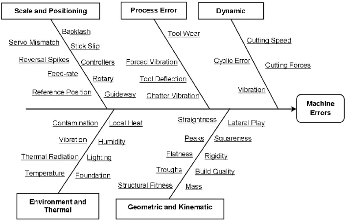
positioning errors are influenced by many error sources which include environmental factors, machine components and assembly inaccuracies and machining process dynamics. The typical error sources are listed in Figure 2.3.

Figure 2.3: Ishikawa diagram with machine error sources (Jamshidi, Maropoulos, Chappell, & Cave, 2015) based on (Lamikiz et al., 2009)

Ramesh et al. defined two most significant error sources (Ramesh, Mannan, & Poo, 2000) as: 1) Quasi-static errors – related to the machine structure: kinematic, geometric and thermal

errors

2) Dynamic errors – caused by the spindle error motion, vibrations of the machine structure, controller errors

Machine geometric error

Geometric errors in machine structure are the most significant error sources and result in position and orientation inaccuracies of the tool and workpiece (volumetric error) (Abbaszadeh-Mir, Mayer, Cloutier, & Fortin, 2002; Erkan, Mayer, & Dupont, 2011; Seng Khim & Chin Keong, March

(26)

17-19, 2010). Those errors are results of the imperfection of machine components and inaccuracies that occur during the assembly (Ramesh et al., 2000). Geometric errors can be divided into two groups: link error parameters (location errors: joints misalignments, angular offsets, rotary axes separation error) and motion errors (component errors: scale error, straightness error, yaw, pitch, roll of linear axis and angular error, tilts, radial and axial errors of rotary axis) (Abbaszadeh-Mir et al., 2002; Schwenke et al., 2008). The former are position-independent geometric error parameters, the latter are position-dependent (their values change with the position of the axis).

Each axis is affected by 6 motion errors and 5 location errors (Schwenke et al., 2008). In (Ramesh et al., 2000) the link and location errors are showed for the linear and rotary axis correspondingly (Figure 2.4).

2.3 Calibration

Frequent calibrations are crucial for testing and controlling machine precision all along its life in service. Monitoring of machine performance is fundamental for avoiding machining parts that would be rejected after the quality check. Calibration process allows estimating machine geometric errors. They can be used for machine compensation or error correction (Givi & Mayer, 2014), which ensures that the machine is working with the required precision.

For the identification of mentioned geometric errors, different methods and devices are applied. The measurement of geometric errors can be provided using direct and indirect methods (Schwenke et al., 2008). The former gives more detailed information about one of the geometric errors, the latter leads to more complex identification.

Direct methods

Direct methods allow measuring the axis errors without the influence of the other axes and are commonly conducted using laser interferometry techniques (Castro, 2008; Chen, Kou, & Chiou, 1999; Okafor & Ertekin, 2000) or calibrated gauges. When the machine positioning errors are checked, the artefact (e.g., gauge blocks, step gauges) or the laser beam are aligned with the machine axis.

(27)

(28)

Laser interferometry is one of the most accurate methods but requires expensive equipment, trained operator and may be time consuming. Through direct measurements, the positioning, straightness, angular and squareness errors can be measured separately. Figure 2.5 shows the laser interferometer alignment for the measurement of the Y-axis positioning error. The laser head is situated outside the machine, the interferometer is set on the machine table and reflector is attached to spindle. During the measurement X and Z axes are locked. The readings from the CNC machine and laser interferometer are registered for the same positions and then compared. The difference between them is used to calculate the positioning error.

Figure 2.5: Y-axis position error measurement using laser interferometry (Schwenke et al., 2008)

Indirect methods

Indirect methods identify errors using different measuring devices, such as ball-bar (Jae Pahk, Sam Kim, & Hee Moon, 1997), various calibrated 2- and 3-D artefacts (Bringmann, Kung, & Knapp, 2005; Lei & Hsu, 2003), laser trackers (Aguado, Samper, Santolaria, & Aguilar, 2012; Linares et al., 2014) and laser-tracer (Moustafa, Gerwien, Haertig, & Wendt, 2009; Schwenke, Schmitt, Jatzkowski, & Warmann, 2009), “chase the ball” calibration (Bringmann & Knapp, 2006; Zargarbashi & Mayer, 2009) or an uncalibrated artefact probing (Mayer, 2012).

In order to identify geometric errors using indirect methods, the machine kinematic model needs to be built. The detailed procedure of error modeling and identification is presented in (Mir et al., 2002). The main steps are:

(29)

1) Building a direct kinematic model of the machine

The kinematic model represents the relative location of a workpiece W and tool T to the machine frame F. It can be described by using the homogenous transformation matrices (HTM) (Mir et al., 2002).

2) Generating Jacobian matrix

The sensitivity Jacobian matrix 𝐉 represents the changes in the tool position 𝛿𝝉 relative to the workpiece (volumetric error (Seng Khim & Chin Keong, March 17-19, 2010)) caused by the small changes in the machine error parameters 𝛿𝒚:

𝛿𝒆𝑣 = 𝑱 ∙ 𝛿𝒚 (2.1)

The Jacobian matrix can be obtained from the HTMs.

3) Identifying unknown geometric error parameters geometric

To identify the parameters the Jacobian matrix 𝑱 is calculated for different workpiece and tool position. Therefore the eq. (2.1) becomes:

𝛿𝒚 = 𝑱+_{∙ 𝛿𝒆}

𝑣 (2.2)

where 𝑱+ _{is a pseudoinverse matrix of 𝑱.}

One of the devices that allow efficient volumetric error measurement and estimating machines errors is the ball-bar (Abbaszadeh-Mir et al., 2003; Jamshidi et al., 2015; Lee & Yang, 2013). Pahk et al. (Jae Pahk et al., 1997) used the kinematic ball-bar (Figure 2.6) to measure the volumetric error. The circular error measurement were conducted on the machine tool and the variations of the ball-bar length were registered. The authors developed a model that allowed identifying machine parametric errors: positional, straightness, angular, and backlash.

(30)

Figure 2.6: Error measurement using the kinematic ball-bar (Jae Pahk et al., 1997)

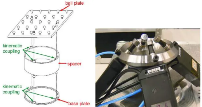
Bringmann et al. (Bringmann et al., 2005) proposed a calibrated pseudo-3D-artefact (Liebrich, Bringmann, & Knapp, 2009) for a calibration of a three-axis machine tool, a CMM or a robot. The artefact was obtained from the 2D-ball plate placed on the kinematic coupling mounted on the base plate or on a spacer (Figure 2.7 left). The measurement of the ball positions with the four linear probes system (Figure 2.7 right) in different configurations of the artefact allowed eliminating the CMM errors that were not influencing the calibration of the artefact.

Figure 2.7: left: Schematic configuration of the pseudo-3D-artefact; right: linear displacement measurement system with four sensors(Bringmann et al., 2005)

(31)

The indirect methods can be conducted using the laser techniques. Schwenke et al. (Schwenke et al., 2009) used a tracking interferometer (laser tracer), which beam tracks the reflector (mounted on the machine head). It allowed registering the length measurements and comparing them to the nominal ones. Those differences introduced in the machine kinematic model led to the machine linear and rotary axes errors estimation.

“Chase the ball” or cap-ball model based calibration was performed by Bringmann et al. (Bringmann & Knapp, 2006) and (Zargarbashi & Mayer, 2009). This method requires mounting the ceramic ball in the machine spindle and measuring its position changes during the axes movement with the trajectory that maintains the same nominal position of the tool and workpiece. The tool and workpiece position differences are measured using four linear sensors (Bringmann & Knapp, 2006) or three capacity sensors (Zargarbashi & Mayer, 2009). The latter configuration is presented in Figure 2.8.

Figure 2.8: Cap-ball measurement system (Zargarbashi & Mayer, 2009)

Viprey et al. (Viprey, Nouira, Lavernhe, & Tournier, 2016) designed a calibrated multi-feature bar that consists in a repetition of a pattern (four flat surfaces and three cylinders). Aligning the artefact with the linear axes of a three-axis machine tool and measuring features of the proposed bar led to the estimation of twenty one geometric errors.

(32)

However, the machine tool calibration can be performed with an uncalibrated artefact. Erkan et al. (Erkan, 2010; Erkan et al., 2011) used uncalibrated master ball artefact (RUMBA) to identify machine geometric error parameters. The proposed artefact consists of master balls mounted at the tips of rods, with different lengths, screwed onto the machine table (Figure 2.9). The artefact is reconfigurable and does not need calibration, what makes the measurement faster and easier to conduct. During the test, the balls centers are measured in different angular axes indexations in order to obtain the value of the volumetric error. The analysis of the position measurement of each ball and the whole artefact allows separating the impact of the rotary and linear axes on the volumetric error.

Figure 2.9: Artefact configuration on five-axis machine (Erkan et al., 2011)

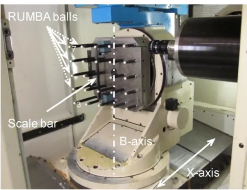
Scale enriched master ball artefact (SAMBA) (Mayer, 2012) method is very similar to the RUMBA and can be conducted for various number of master balls (up to twenty four - Figure 2.10) with different calibration strategies (Mchichi & Mayer, 2014). The presence of a calibrated scale bar (which has to be measured at least once) allows estimating the scale errors of the linear axis. In (Mayer, 2012), SAMBA method was used to identify ten location errors (Figure 2.11) and three scale errors. The estimated machine geometric error parameters are listed in Table 2.1. along with their descriptions and both symbols used in (Mayer, 2012) and in this thesis.

(33)

Figure 2.10: SAMBA artefact with twenty four master balls mounted on the machine tool (Mayer, 2012)

(34)

Table 2.1: Estimated machine geometric error parameters (Mayer, 2012)

Symbol (Mayer, 2012)

Symbol in

this thesis Description

AOB EAOB out-of-squareness of the B-axis relative to the Z-axis (rad)

COB ECOB out-of-squareness of the B-axis relative to the X-axis (rad)

XOC EXOC distance between the B and C axes (m)

AOC EAOC out-of-squareness of the C-axis relative to the B-axis (rad)

BOC EBOC out-of-squareness of the C-axis relative to the X-axis (rad)

BOZ EBOZ out-of-squareness of the Z-axis relative to the X-axis (rad)

AOY EAOY out-of-squareness of the Y-axis relative to the Z-axis (rad)

COY ECOY out-of-squareness of the Y-axis relative to the X-axis (rad)

XOS EXOC1 X offset of the spindle relative to the B-axis (m)

YOS EYOC1 Y offset to the spindle relative to the C-axis (m)

EXX EXX positioning linear error term of the X-axis (m/m)

EYY EYY positioning linear error term of the Y-axis (m/m)

EZZ EZZ positioning linear error term of the Z-axis (m/m)

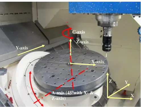
Another example of a calibration without a calibrated artefact was presented in Figure 2.12 (Mayer, Rahman, & Los, 2015). This method uses an uncalibrated cylindrical indigenous artefact (machine table) and allows estimating machine inter-axis errors. It requires mounting a touch probe in the spindle head and probing a number of points on around and on the machine table in different rotary axis indexations.

(35)

Figure 2.12: Indigenous artefact probing on the wCAYFXZ(C1)t machine tool (Mayer et al., 2015)

Standards

The available standards for the machine tool testing give the guidance on the machine testing using the direct methods and the measuring equipment with a high precision, e.g., laser interferometer. ISO 230-2 (ISO, 230-2:2014) and ASME B5.54 (ASME, B5.54:2005) standards describe procedures for the measurement of the machine geometric errors and their repeatability of the results through the repeated uni- and bi-directional tests. The significant difference of testing the machine according to those standards is that ISO 230-2 requires a warm-up test before the measurement, while ASME B5.54 excludes it. However, both standards do not consider the indirect calibration methods.

2.4 Calibration results evaluation

Once the information about the machine geometry is known and the calibration results are estimated, a decision to/not to use them for compensation or apply a software correction has to be made. This decision has a direct impact on the machine precision, thus the calibration results should be evaluated. C-axis X Y Z Y-axis Z-axis X-axis

A-axis (450_{with X- &}

(36)

In the literature, examples of calibration results evaluation through the predicted volumetric error (Liang, Chen, Chen, Sun, & Chen, 2013) or the workpiece feature errors (Bringmann, Besuchet, & Rohr, 2008) can be found. However, this thesis focuses on the calibration as a measurement process, therefore the calibration uncertainty estimation is studied.

Uncertainty estimation

The uncertainty is a “non-negative parameter characterizing the dispersion of the quantity values being attributed to a measurand, based on the information used” (GUM, Joint Committee for Guides in Metrology, JCGM 200:2012). Every measurement result should be presented with its uncertainty. The direct calibration methods results uncertainty is typically estimated as the uncertainty of, for example, the laser displacement measurement. The indirect methods, due to their complex models, usually lead to the application of the Monte Carlo method (MCM) for the uncertainty assessment. In general, Monte Carlo method requires sampling the input quantity possible values, using obtained samples to compute the results and aggregating the results. In uncertainty estimation, the input quantity samples are obtained from their distribution and the calculated output values give the estimate of the result distribution. Thus, the uncertainty can be calculated.

Lira et al. (Lira & Grientschnig, 2010) proposed a method that estimates the uncertainty of positional deviations of a machine tool when the calibration is performed according to the ISO 230-2 standard (ISO, 230-2:2014). This approach included in the uncertainty budget: the measurand (position) variations, temperature, measuring device alignment and resolution. Those uncertainties were propagated on the estimate machine positional accuracy results using the law of propagation of uncertainties.

The test conditions and their impact on the positioning measurement used for direct calibration was analyzed by Knapp (Knapp, 2002). The author pointed out that, in practice, the calibration is performed in a workshop not in laboratory conditions, and the test uncertainty should not be propagated only from the measuring device uncertainty. The non-optimal conditions were amplified in the uncertainty propagation in order to demonstrate that uncertainty results, obtained for example, only from the laser interferometer displacement, may not reflect the reality.

(37)

Santolaria et al. (Santolaria & Ginés, 2013) applied MCM to estimate the uncertainty on the robot arm calibration results. The input uncertainty includes the length measurement uncertainty. The calibration uncertainty is later propagated on the position and orientation results.

Schwenke et al. (Schwenke, Franke, Hannaford, & Kunzmann, 2005) estimated the uncertainty of six parametric errors from the uncertainty of the laser tracking interferometer measurements modeled as the interferometric length measurement and propagated to the calibration results using MCM. This method included only the uncertainty of the measuring device (laser interferometer). In (Jokiel Jr, Ziegert, & Bieg, 2001) the uncertainty on the calibration of parallel kinematic machines was analysed. The authors pointed the main sources of positioning accuracy errors as the external instrument and the machine itself through the variation of the strut length due to the thermal, geometric and controller influence.

The machine performance changes over the time and their influence on the calibration error were depicted by Parkinson et al. in (Parkinson, Longstaff, & Fletcher, 2014) for the squareness measurement. The authors included, not only the measuring device uncertainty, but also the variations of the straightness errors due to temperature changes. That allowed estimating the uncertainty on the squareness error and developing a calibration automated planning that reduced the uncertainty.

One of the most essential research on the calibration uncertainty was conducted by Bringmann et al. (Bringmann & Knapp, 2009). Through the indirect calibration method the authors showed that machine tool performance has an impact on the calibration results and, including only the uncertainty of the measuring device in the environmental conditions is not sufficient. The Monte Carlo method was applied. The machine performance impact was tested through the introduction in the machine model the geometric errors and simulating the calibration results. The noise added to each error was a random value generated from the uniformly distributed range, which were taken from similar measurements, machine specification or standard values. Thus, the a priori information about the machine tool performance (which is being tested) is required. This methodology for calibration uncertainty estimation was later followed by Ibaraki et al. (Ibaraki, Iritani, & Matsushita, 2013) in a calibration with an artefact of a square column geometry fixed on the machine table.

(38)

Presented methods of calibration uncertainty estimation show that, when it comes to machine tool calibration, there is no common procedure. The Monte Carlo method is widely used for various type of calibration methods and kinematic models (multi-axis machine tools, parallel kinematic machines and robots) uncertainty propagation. However, the necessity for including the machine performance variations in the uncertainty budget has been demonstrated. In all cases of indirect calibration, the uncertainty estimation was performed without considering correlations between the input data, which Haesslbrath et al. (Haesselbarth & Bremser, 2004) consider significant, when similar procedure or an object are measured, and especially when the repeated measurement is being performed. Not including the correlations between the input quantities while using the Monte Carlo method results in sampling the input quantity without considering the interdependencies between them. Thus, it gives less accurate resemblance of the reality. Correlations between the calibration results are not considered either, thus there is no information about the interdependencies between the results. Despite the multi-output calibration model types, the coverage factor for expanded uncertainty is estimated as for a single-output model.

Standards

Estimations of the uncertainty of calibration methods are presented in the ISO 230-2 standard (ISO, 230-2:2014). However, it is only for the indirect calibration method shown in the standard using a calibrated component (laser interferometer). In this case, the law of propagation of uncertainty can be adapted and applied.

Joint Committee for Guides in Metrology (JCGM) is one of the international organizations of Bureau Interantional des Poids et Mesures (BIMP). JCGM produced a series of documents “Evaluation of measurement data”. The “Guide to the expression of uncertainty in measurement” (GUM) JCGM 100:2008 (GUM, Joint Committee for Guides in Metrology, JCGM 100:2008) states the general rules of the measurement uncertainty and the GUM Supplement 1 (GUM S1) JCGM 101:2008 (GUM, Joint Committee for Guides in Metrology, JCGM 101:2008) allows calculating the uncertainty of measurements with an arbitrary model through the Monte Carlo method (MCM). Both of those approaches (GUM and GUM S1) are limited to single output models. The uncertainty on multi-output models can be propagated using the MCM or GUM uncertainty framework (GUF) as described in the GUM Supplement 2 (GUM S2) JCGM 102:2011 (GUM, Joint Committee for Guides in Metrology, JCGM 102:2011).

(39)

Finally, the JCGM 107 (GUM, Joint Committee for Guides in Metrology, JCGM 107:In preparation) as it is described in JCGM 104 (GUM, Joint Committee for Guides in Metrology, JCGM 104:2009) provides guidance in the evaluation of the uncertainty when least-square models are used to estimate parameters of the calibration function. The necessity of evaluating and taking into account the uncertainty structure (the standard uncertainties and covariances of the measured quantities) is expressed. Unfortunately, according to the latest JCGM Working Group 1 News brochure ((BIPM), 2017), JCGM 107 is not available yet and should be developed at a later stage. The standards for machine performance testing and uncertainty estimation show the need, complexity and challenges of the calibration uncertainty estimation but has yet to give the specific guidance when least-square model is used in an indirect calibration with uncalibrated artefact.

2.4.2.1 Adaptive Monte Carlo method

The Monte Carlo method described in GUM S2 (GUM, Joint Committee for Guides in Metrology, JCGM 102:2011) allows propagating the uncertainty sources on the measurement result without the analytical representation of a measurement model. In general, the MCM requires sampling the distributions of the input quantity and introducing these sets of random (with the distribution) values into the model, so that the range of the output values can be calculated. The detailed (adaptive) Monte Carlo approach for SAMBA method applied in the presented research is to be described in Chapter 4.

MCM method according to GUM S2 has been applied by Eichstadt et al. (Eichstadt, Link, Harris, & Elster, 2012) in an uncertainty evaluation of a dynamic measurement, in which the knowledge about the measuring system is limited. Conducting the MCM allowed avoiding linearization of the model, which could significantly influence the magnitude of the errors, and calculating the coverage regions for a multi-output model.

2.4.2.2 GUM uncertainty framework

GUM S2 gives the opportunity to estimate the uncertainty of a multi-output model using the GUM uncertainty framework (GUF). This approach requires calculating the partial derivatives of the output quantities to the input quantities. When the measurement models have the iterative solution or cannot be expressed analytically, the partial derivatives may be estimated experimentally or

(40)

numerically. The detailed GUF methodology is to be presented in Chapter 6 and its validation with MCM in Chapter 7.

(41)

CHAPTER 3 GENERAL PRESENTATION

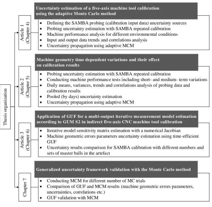
The introduction (Chapter 1) and the literature review (Chapter 2) shaped the thesis subject. This chapter presents the overall structure with the article overview. The following three chapters corresponds to three (two journal and one conference) articles. In Chapter 7 additional results are presented. Those chapters show the main doctoral research. The thesis dissertation ends with a general discussion (Chapter 8) and conclusion (Chapter 9).

All tests and calculations presented in this thesis were conducted on a five-axis machine tool using the SAMBA calibration method, which has a multi-input, multi-output model with iterative solution and (scale enriched) uncalibrated artefact.

The article entitled “Uncertainty estimation of a five-axis machine tool calibration using the adaptive Monte Carlo method”, which was submitted in March 2017 to Precision Engineering Journal, is in Chapter 4. The research work, presented therein, is exploring the possibility of calculating the uncertainty of the calibration method that uses the uncalibrated artefact. Moreover, the machine performance and its variations due to the different environmental conditions are analysed. The following uncertainty sources are considered: the artefact variations occurring during the test, the probe repeatability and the machine itself. Thus, the measurand (machine geometry) is, at the same time, the source of the calibration uncertainty. In order to include all those factors, the repeated measurements (over 24 hours) are proposed as the estimation of the probing uncertainty (input quantity). That way, standard deviations, covariance and distributions are obtained and propagated through the (adaptive) MCM method on the calibration results (output quantity). The results with their expanded uncertainties are compared for different environmental conditions.

Chapter 5 is constituted of the article “Machine geometry time dependent variations and their effect on calibration results”, which was submitted in March 2017 to Measurement. In this paper, the machine performance changes are analysed. However, this time the focus is on short- and medium- term variations. In the previous paper, it was established that the machine changes occur during one day. But do the machine tool varies between the days? To answer this question, the SAMBA calibration was repeated on the machine four times a day over five days. That allows comparing the mean and variances obtained for each day. Moreover, the trend in the probing and calibration results is discussed.

(42)

Chapter 6 presents the paper “Application of GUF for a multi-output iterative measurement model estimation according to GUM S2 in indirect five-axis CNC machine tool calibration”, which was presented during the XI LAMDAMAP 2015 conference and published in the proceedings Laser Metrology and Machine Performance XI, in March 2015. MCM has many advantages. It does not require the analytical function of the measurement model or its linearization. Moreover, distributions of the estimated parameters are obtained. However, depending on the number of MC trials and based on a single trial running time, it can be time-consuming. GUF allows estimating the uncertainties faster but it requires the sensitivity Jacobian matrix of the output quantity to the input quantity. Since SAMBA has an iterative solution to the least square method the Jacobian cannot be established analytically. Thus, it is estimated with the numerical Jacobian. Then, the GUF method is used to calculate the uncertainties on the calibration results for different number of master balls present in the artefact.

Finally, in Chapter 7 the validation of time-efficient GUF with the MCM is presented. The estimated parameters, their uncertainties, covariance matrices and the coverage factors are compared for both methods. The MCM simulation results are calculated for different numbers of MC trials in order to show its impact on the obtained values.

(43)

T he si s or ga ni za ti on A rt ic le 1 (C ha pt er 4 ) A rt ic le 2 (C ha pt er 5 ) C hapt er 7 A rt ic le 3 (C ha pt er 6 )

 Defining the SAMBA probing (calibration input data) uncertainty sources  Probing uncertainty estimation with SAMBA repeated calibration

 Machine performance analysis for different environmental conditions  Input and output data trends and correlations analysis

 Uncertainty propagation using adaptive MCM

 Probing uncertainty estimation with SAMBA repeated calibration

 Conducting machine performance tests including short- and medium- term variations  Daily means, variances, trends and correlations analysis of probing data and

calibration results

 Pooled (by days) uncertainty estimation  Uncertainty propagation using adaptive MCM

 Conducting MCM for different number of MC trials

 Comparison of GUF and MCM results (machine geometric errors parameters, uncertainties, correlations etc.)

 GUF validation with MCM

 Iterative model sensitivity matrix estimation with a numerical Jacobian

 Machine geometric errors parameters uncertainty estimation using time-efficient GUF

 Uncertainty results comparison for SAMBA calibration with different numbers and sets of master balls in the artefact

Uncertainty estimation of a five-axis machine tool calibration using the adaptive Monte Carlo method

Machine geometry time dependent variations and their effect on calibration results

Application of GUF for a multi-output iterative me asurement model estimation according to GUM S2 in indirect five-axis CNC m achine tool calibration

Generalized uncertainty framework validation with the Monte Carlo method

(44)

CHAPTER 4 ARTICLE 1: UNCERTAINTY ESTIMATION OF

A FIVE-AXIS MACHINE TOOL CALIBRATION USING

THE ADAPTIVE MONTE CARLO METHOD

A. Los, J.R.R. Mayer

Department of Mechanical Engineering, Polytechnique Montreal, Montreal, QC, Canada

* Submitted to Precision Engineering in March 2017

4.1 Abstract

Calibration of the geometry of five-axis machine tools needs to be performed periodically since the machine accuracy has a direct impact on machined parts. Because mechanical adjustment and a software correction may be done using calibration results, the measurement results must be evaluated. In this paper, the scale and master ball artefact (SAMBA) method is evaluated through the estimation of the uncertainty of the identified machine geometric error parameters. This approach has the multi-input multi-output (MIMO) model and an iterative solution that makes it challenging to apply commonly used uncertainty calculation methods. The Guide to the Expression of Uncertainty in Measurement Supplement 2 (GUM S2) gives the opportunity to estimate the uncertainty of a MIMO model through the adaptive Monte Carlo method (MCM). The uncertainty is propagated from the repeated calibration tests conducted in different conditions. The uncertainties are calculated for each of the identified machine geometric error parameters along with their covariance. The correlations between the output variables and the impact of the machine conditions before and during the calibration are analyzed. The results demonstrate machine tool performance impact on the calibration results.

Keywords: machine tool, calibration, SAMBA, Monte Carlo, uncertainty.

4.2 Introduction

The calibration of a machine tool requires estimating the geometric error parameters of its linear and angular axes. Schwenke et al. [1] described and classified different methods for machine tool calibration into two groups: direct and indirect methods. The former allow measuring the axis

(45)

errors without the influence of the other axes and are commonly conducted using laser interferometry techniques [2, 3]. The latter identify errors using different measuring devices, such as ball-bar [4], various 2- and 3-D artefacts [1, 5-7], laser trackers [8] and laser tracer [9] or an uncalibrated artefact probing [10].

Once the estimates of the geometric error parameters have been obtained, the decision of using them for a correction and/or compensation must be made. That is why the calibration results should be evaluated. One of the evaluation methods can be conducted through the predicted (with and without calibration) workpiece feature errors as Bringmann et al. proposed in [11], that allowed choosing the most optimal calibration method. The estimated calibration results can also be evaluated through their uncertainty as any other kind of measurement result. Since the measurement models used in the indirect methods are complex and are multi-input multi-output, the GUM uncertainty framework (GUF) for a single output presented in GUM [12] cannot be conducted.

Bringmann et al. [13] estimated the uncertainties on the machine geometric error parameters of the model-based indirect calibration method, called “chase the ball”, using general Monte Carlo method (MCM). This approach requires adding noise to the geometric errors in the simulated machine model. The noise values are chosen arbitrarily from standards or machine specifications without considering correlations between them or the obtained calibration results. The authors also depicted that the machine performance has a significant impact on the calibration results. Other researchers also applied MCM based on GUM Supplement 1 (GUM S1) [14]. Andolfatto et al. [15] used the adaptive MCM to estimate uncertainty on machine tool axis location errors with the confidence intervals. Santolaria et al. [16] conducted robot kinematic calibration and estimated, through simulation, the uncertainty on the calibration results. Schwenke et al. [17] estimated the uncertainty on six parametric errors of the Y-axis of a coordinate measuring machine (CMM) and on a milling machine. The machine errors are identified using a laser tracer. The displacement measurements noise is estimated as normally distributed random numbers without considering the correlation between the input data. All of the previously mentioned approaches use the MCM for a multi-output model but do not consider the full uncertainty structure (standard uncertainties and covariance of the measured data) (JCGM 104:2009 6) [18], nor the coverage factor associated with the number of the estimated parameters.

(46)

The indirect calibration methods allow estimating many geometric errors simultaneously. That is why the covariance between them should also be considered when the uncertainties are calculated. Moreover, the coverage factor should be based not only on the desired coverage probability but on the number of output values as well. The opportunity of calculating the uncertainty on the multi-output model results is given in GUM S2 [19]. It has been applied by Eichstadt et al. [20] to an efficient uncertainty estimation in a challenging case of dynamic measurement. The MCM uncertainty estimation results are compared with two other memory-efficient approaches.

In this paper, the machine geometric errors are identified using the SAMBA [10] method, whereby the volumetric observations are gathered using an uncalibrated artefact made of a number of spheres, a calibrated fixed length ball bar (scale bar) and a touch trigger probe mounted in the machine tool spindle. The machine, with its axis location and linear axis positioning error gains, is modeled using rigid body kinematics so that its geometric error parameters can be estimated. This method is based on a multi-output model – all the machine geometric errors are calculated simultaneously from the volumetric measurement indications (probing data). In this paper, since the SAMBA method is based on multistage and iterative calculations, analytical procedures are not easily conducted. Thus the adaptive MCM [19] is followed. The uncertainties for the probing data are estimated from the repeated measurement conducted under different measurement conditions (with and without the warm-up cycle). The warm-up cycle performed before the measurement allows simulating the machine working conditions [21] and is required when the calibration (using direct methods) is following the ISO 230-2 standard [22]. However, the ASME B5.54 standard [23] (for indirect methods) do not require a warm-up cycle and the errors due to machine heat sources are not present prior to the tests [21]. Conducting the calibration series with and without the warm-up cycle allows demonstrating the machine performance influence on calibration results depending on the calibration pre-conditions.

4.3 SAMBA calibration method

Artefact probing

The SAMBA method allows estimating the machine geometric error parameters from the probing (using a touch probe mounted in the spindle) of a number of master balls (mounted on rods with different lengths) in different machine rotary axis indexations and a scale bar (probed at least once).

(47)

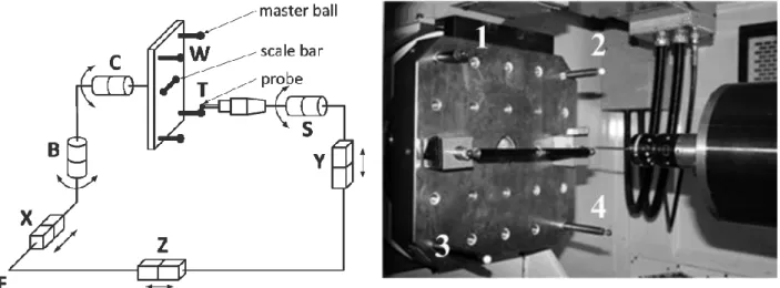
The SAMBA artefact with the four master balls and the scale bar (which is the only calibrated component) mounted on the machine table is depicted in Figure 4.1 (right). For each indexation, each of the balls is probed in five points, which allows calculating the X-, Y- and Z-axis readings corresponding to positioning the stylus tip at the ball center and comparing it with its nominal position.

Herein, the experimental data is collected using a HU40-T model five-axis machine tool made by Mitsui Seiki. Its topology is depicted in Figure 4.1 (left). The analyzed machine is modeled using eleven joint link errors with values estimated during previous calibration [10].

Figure 4.1: left: Five-axis CNC machine model with the topology WCBXFZY(C1)T; W - workpiece, T - tool, F - machine foundation, B, C – rotary axes around the Y and Z axes respectively, X, Y, Z – machine linear axes, S – spindle; right: SAMBA artefact being probed

using the Renishaw probe MP700 on a Mitsui Seiki HU40-T machine tool

Parameters identification

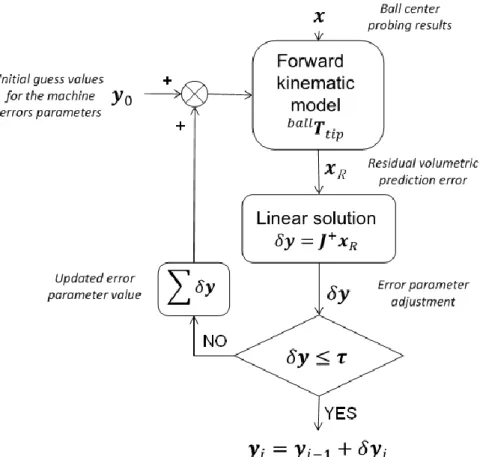
The identification of the geometric error parameters, presented in Figure 4.2, requires building the kinematic model of the machine, that allows calculating the predicted tool position 𝑷_𝑡𝑖𝑝 [24] relative to the probed ball center position 𝑷_{𝑏𝑎𝑙𝑙} using the measured axis positions. At measurement, the two positions coincide virtually (not physically since the probe tip cannot be positioned at the center of the ball):

(𝑷_𝑡𝑖𝑝− 𝑷_{𝑏𝑎𝑙𝑙})_{𝑎𝑐𝑡𝑢𝑎𝑙} ≡ [0, 0, 0]𝑇

(48)

Figure 4.2: SAMBA identification flow chart

The Newton-Gauss approach is used to estimate the changes to the machine geometric error parameters in order to reduce the error between the prediction of the model and the observation:

(𝑷_𝑡𝑖𝑝− 𝑷_{𝑏𝑎𝑙𝑙})_{𝑝𝑟𝑒𝑑𝑖𝑐𝑡𝑒𝑑}+ 𝑱 ∙ 𝛿𝒚 = 0 _(4.2)

where:

𝑱 is the sensitivity Jacobian matrix (of the residuals 𝒙𝑅 to 𝛿𝒚) and 𝛿𝒚 is the column matrix of the

adjustment in machine parameters and the artefact geometry and dimension. With:

(𝑷𝑡𝑖𝑝− 𝑷𝑏𝑎𝑙𝑙)_{𝑝𝑟𝑒𝑑𝑖𝑐𝑡𝑒𝑑}= 𝒙𝑅 (4.3)

(49)

𝑱 ∙ 𝛿𝒚 = −𝒙_𝑅 (4.4) Finally, we obtain:

𝛿𝒚 = 𝑱+_{∙ (−𝒙}

𝑅) (4.5)

where 𝑱+ is a pseudoinverse matrix of 𝑱 and 𝒙_𝑅 is predicted and extracted from the homogenous transformation matrix 𝑏𝑎𝑙𝑙𝑻_𝑡𝑖𝑝: 𝒙_𝑅 = 𝑏𝑎𝑙𝑙𝑻_𝑡𝑖𝑝[ 0 0 0 1 ] (4.6)

keeping only the top three components. For the analyzed five-axis machine, 𝑻_𝑡𝑖𝑝 𝑏𝑎𝑙𝑙 _{= ( 𝑻} 𝑋0 𝑻𝑋 𝑋0 _𝑻 𝑋′ 𝑋 _𝑻 𝐵0 𝑋′ _𝑻 𝐵 𝐵0 _𝑻 𝐵′ 𝐵 _𝑻 𝐶0 𝐵′ _𝑻 𝐶 𝐶0 _𝑻 𝐶′ 𝐶 _𝑻 𝑏𝑎𝑙𝑙 𝐶′ 𝐹 ₎−1_∙ ∙ 𝑇𝑍0 𝑻𝑍 𝑍0 _𝑻 𝑍′ 𝑍 _𝑻 𝑌0 𝑍′ 𝑻𝑌 𝑌0 _𝑻 𝑌′ 𝑌 _𝑻 𝑆0 𝑌′ 𝑻𝑆 𝑆0 _𝑻 𝑡𝑖𝑝 𝑆 𝐹 (4.7)

where, for example: 𝑻_𝐵₀

𝑋′

= 𝑰 (4.8)

is the homogenous transformation matrix of the nominal B-axis location relative to the actual X-axis carriage, while: 𝑻𝐵 𝐵0 _{= [} 𝑐𝑜𝑠 𝑏 0 0 1 𝑠𝑖𝑛 𝑏 00 0 −𝑠𝑖𝑛 𝑏 0 0 0 𝑐𝑜𝑠 𝑏 00 1 ] (4.9)