STOCHASTIC STABILITY OF A TOWER CRANE UNDER GUSTY WINDS

STOCHASTIC STABILITY OF A TOWER CRANE UNDER GUSTY WINDS Hélène VANVINCKENROYEa, Thomas ANDRIANNEb, Vincent DENOËLa

a

Structural and Stochastic Dynamics, University of Liège – Belgium b

Wind Tunnel Lab, University of Liège – Belgium [email protected]

Abstract

These instructions give the author basic guidelines to prepare the extended version of their accepted abstracts to be included in the Conference Proceedings. You are kindly asked to read and follow them carefully as the reproduction of your paper will be made directly from this text.

Keywords: First passage time, wind tunnel, tower crane, stochastic stability, Mathieu oscillator

INTRODUCTION

Tower cranes are engines designed to transport heavy weights. Over the last years, a large number of crane collapses has been recorded and reported in the media, e.g. in New-York in 2012 under storm Sandy (Figure 1). Many others are available on dedicated websites [1, 2].

Figure 1. Crane failure in New-York, 2012 [1].

Although the behavior of cranes is a widely studied problem in the literature, most research works focus on the study of structures in use, i.e. during lift operations [3, 4]. As tower cranes are high-rise and lattice structures, wind is an important excitation. In case of high wind velocities, the crane is out-of-service and left free to rotate as a weathervane in order to avoid overturning of the structure. The corresponding out-of-service wind speed is studied in [5, 6, 7]. In opposition with all the previous research about tower cranes in use, Voisin performed experimental analysis in order to understand and characterize other crane instabilities under wind excitation and determine the

susceptibility of a tower crane to autorotation when it is out-of-service. This experiment consists in the determination of a probability of autorotation of the jib in a given environment. This method allows to validate or not a configuration by experimental campaigns [8, 9]. A wide variety of tools already exists concerning wind loading, stochastic processes, dynamic analysis of structures and can be combined to analyze and better understand the behavior of tower cranes in a stochastic wind velocity field.

A conceptual model of this problem will help catching the impact of the different geometrical, structural and wind parameters and their effect on autorotation. In this perspective, the crane is here represented by a single degree-of-freedom model composed of a rigid jib rotating around a fixed pivot [10]. This mechanism is similar to a pendulum. As the wind loading depends on the angular position and velocity of the crane through aerodynamic forces and pressure coefficients, the wind excitation is called autoparametric which is a characteristic of the pendulum as well. Assuming no damping, the dimensionless governing equation of this system submitted to an external force w(t) and a parametric force u(t) is given by:

𝑥̈ + ξ 𝑥̇(1 + 𝑢(𝑡)) 𝑥 = 𝑤(𝑡). (1)

The rewriting of the governing equation under this format enlarges the applicability of the study to other similar problems. For instance a vertical motion of the support of a pendulum in the gravity field generates this kind of parametric excitation while a horizontal motion generates a forcing excitation [11, 12]. As another example, the rolling-motion of a ship under wave excitations is

described by a similar Mathieu equation and finds a direct application in the extraction of energy [13]. The stochastic stability of an oscillator is evaluated in this work through the first passage time, which is the time required by the system to evolve from a given state to another one [10]. Considering a slightly damped oscillator submitted to a white-noise parametric and forced excitation of small intensity 𝑆_𝑢 and 𝑆_𝑤 , it can be shown that the energy evolves on a slower time-scale than the position or rotational velocity, and the system is therefore called quasi-Hamiltonian. Through time-scale separation and stochastic averaging, the average first passage time 𝑡₁ given by the solution of the Pontryagin equation takes the following closed-form expression, in the undamped case

(𝜉 = 0): 𝑡1 = 4 𝑆𝑢ln ( 𝐻𝑐𝑆𝑢+2𝑆𝑤 𝐻0𝑆𝑢+2𝑆𝑤), (2)

with 𝐻0 the initial energy level, 𝐻𝑐 = 𝐻0+ Δ𝐻 the target energy. This expression highlights the fact that the first passage time is depending on the energy only, and not on the rotational position or velocity. For a better analysis of the expression, the first passage time is rewritten as a function of the reduced energy 𝐻∗ =𝐻𝑆𝑢

2𝑆𝑤, so that Equation (2) becomes:

𝑡1(𝐻) = 4

𝑆𝑢ln (1 +

Δ𝐻∗

𝐻0∗+1), (3)

Expression (3) highlights the existence of three different regimes [10].

First, in the Incubation regime (I), for Δ𝐻∗≪ 𝐻₀∗+ 1, the logarithm may be linearized and the mean first passage time can be written as 𝑡1 ≈

4 𝑆𝑢

Δ𝐻∗

𝐻0∗+1 . The first passage time is then proportional to

Δ𝐻∗ . This is valid for 𝑡1 ≪ 4

𝑆𝑢 so that an incubation time is arbitrarily defined as 𝑡𝑖𝑛𝑐𝑢𝑏 =

1 2𝑆𝑢

corresponding to the duration of linearly increasing energy. Otherwise, if Δ𝐻∗ _{≳ 𝐻}

0∗+ 1, the logarithm cannot be linearized, and the expected first passage time is of the order of the incubation time or more.

Second, in the Multiplicative regime (M), 𝐻₀∗ _{≫ 1 and the expected first passage time required} to go from a relatively large initial energy level to an even much larger energy level tends to

4

𝑆𝑢ln (1 +

Δ𝐻∗

𝐻0∗) . It therefore depends on by how much the initial energy is multiplied to obtain the

target energy level. In the overlap with the incubation regime, the logarithm can be linearized and one finds 𝑡₁ ≃ 4 𝑆𝑢 Δ𝐻∗ 𝐻₀∗ = 4 𝑆𝑢 Δ𝐻 𝐻0 .

Third, in the Additive regime (A), 𝐻₀∗ ≪ 1 and the first passage time tends to 4

𝑆𝑢ln(1 + Δ𝐻

∗_). In this latter case, no matter the smallness of the initial energy 𝐻₀ in the system, provided it is much smaller than 2𝑆𝑤

𝑆𝑢, it does not influence the expected first passage time. In this regime, the expected first

passage time only depends on the increase in energyΔ𝐻∗. In the overlap with the incubation regime, the logarithm can be linearized and one finds 𝑡₁ ≃ 4

𝑆𝑢Δ𝐻

∗ ₌ 2Δ𝐻 𝑆𝑤.

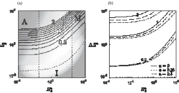
Figure 2 (a) presents the ratio 𝑡1 𝑆𝑢 4 = ln (1 + Δ𝐻∗ 𝐻₀∗+1) as a function of Δ𝐻 ∗ _{and 𝐻} 0∗ and identifies the three regimes (incubation, additive and multiplicative). The curves of same expected first passage time are regularly spaced for values smaller than 0.1, which correspond to the incubation regime where the time increases linearly with the energy increase. The upper left corner corresponding to the additive regime presents horizontal asymptotes as the first passage time is independent of the initial energy level. Finally, the multiplicative regime is represented in the upper right corner where the time depends on the proportional energy increase Δ𝐻∗/𝐻₀∗ and the curves present a unitary slope in

logarithmic scales.

(a) (b)

Figure 2 – (a) Representation of the average first passage time with identification of the three regimes for 𝜉 = 0. (b) Representation of the average first passage time for three different values of the damping coefficient. Similarly, the average first passage time of the damped oscillator is given by [10]:

𝑡₁ = 4 𝑆𝑢(1−𝑎)(ln (1 + Δ𝐻∗ 𝐻0∗) + (1+𝐻0∗+Δ𝐻∗)𝑎−(1+𝐻0∗)𝑎 𝑎 − ∫ (1+𝑡)𝑎 𝑡 𝑑𝑡 𝐻0∗+Δ𝐻∗ 𝐻₀∗ ), (4)

with 𝑎 =8𝜉

𝑆𝑢. The three different regimes are also identified in [10] through asymptotic analysis of

expression (4). Figure 2 (b) shows the reduced expected first passage time for non-zero damping ratios. It is seen that the damping ratio has little influence on the first passage time in the incubation regime, while it extends the expected first passage time in the additive regime. In the multiplicative regime (upper right corner), the damping ratio changes the slope of the curve of equal first passage time, which means that the first passage time is governed by a power of Δ𝐻∗_/𝐻

0∗ smaller than unity. In all regimes, increasing the damping ratio increases the first passage time.

The average first passage time is well-known under its closed-form expression for restricted conditions, such as small white noise excitations, small damping, and linear behavior of the oscillator. Those results have been validated through numerical simulations. The purpose of this work is to perform an experimental analysis of the first passage time of a physical oscillator, in this case a tower crane. The oscillator is submitted to a stochastic space- and time-correlated velocity field that needs to be integrated along the moving jib to provide the resulting torque to take into account into the rotative equilibrium. The experimental tests have been performed in the Wind Tunnel of the University of Liège, in order first to validate the theoretical results obtained through the stochastic model by observation of the different regimes, and second to identify the problem parameters that should be used in order to predict the system behavior with the analytical model developed above.

PROBLEM STATEMENT AND EXPERIMENTAL SETUP

The rotative equilibrium of a crane with inertia 𝐼, damping 𝐶 and rigidity 𝐶 provides the following governing equation:

𝐼𝜃̈ + 𝐶𝜃̇ + 𝐾𝜃 = 𝑀_𝑤, (5)

with the dot representing the derivative relative to time, the wind torque 𝑀_𝑤 = 1

2𝜌𝑎𝑖𝑟𝐶𝑀𝐻𝐵 2_||𝑣

𝑟𝑒𝑙|| 2

= 𝑚∗𝐶_𝑀||𝑣_𝑟𝑒𝑙||2, 𝜌_𝑎𝑖𝑟 the air density, 𝐶_𝑀 the moment coefficient, 𝐻 and 𝐵 the characteristic height and length of the crane, and ||𝑣𝑟𝑒𝑙|| the relative velocity between the jib and the wind. For small incidences, the moment coefficient can linearized so that 𝐶_𝑀 = 𝜕𝐶𝑀

𝜕𝛼 |_𝛼=0𝛼 with 𝛼 the relative angle between the crane and the wind velocity. The wind velocity is defined by its mean component 𝑈 and turbulent components parallel and perpendicular to the mean direction 𝑢₁ and 𝑢₂. To fit with the hypothesis of the stochastic model, the excitations are chosen to be small, of order 𝜖. The relative velocity is given by:

𝑣⃗_𝑟𝑒𝑙 = (𝑈 + 𝑢₁, 𝑢₂) − (−𝑟𝜃̇ sin 𝜃 , 𝑟 𝜃̇ cos 𝜃), (6)

with 𝑟 the distance between the origin of the axis and the aerodynamic center. The variables 𝜃, 𝜃̇, 𝑢₁ and 𝑢₂ are of order 𝜖. Neglecting second orders of 𝜖, corresponding to parametric terms and nonlinear damping, one finds ||𝑣𝑟𝑒𝑙||

2

= 𝑈2+ 2𝑈𝑢1. Similarly, the relative angle is given by 𝛼 = 𝜃 − 𝑣𝑟𝑒𝑙,𝑦

𝑣𝑟𝑒𝑙

,𝑥 ≃ 𝜃 −𝑢2−𝑟𝜃̇

𝑈 . Assuming these simplifications, as well as 𝐾 = 0 as the system has no rigidity, Equation (5) is rewritten as: 𝐼𝜃̈ + (𝐶 − 𝑚∗𝑈𝑟𝜕𝐶𝑀 𝜕𝛼 (1 + 2𝑢̃1)) 𝜃̇ − 𝑚 ∗_𝑈2 𝜕𝐶𝑀 𝜕𝛼 (1 + 2𝑢̃1)𝜃 = −𝑚 ∗_𝑈𝑢 2 𝜕𝐶𝑀 𝜕𝛼 𝜃, (7)

The non-dimensional form is found by introducing the characteristic pulsation Ω defined as Ω2 _{= −}𝑚∗𝑈2

𝐼 𝜕𝐶𝑀

𝜕𝛼 = − 𝑀𝑟𝑒𝑓

𝐼 , the structural damping coefficient 𝜉𝑠 = 𝐶Ω

−𝑀𝑟𝑒𝑓 and the aerodynamic

damping coefficient 𝜉_{𝑎𝑒𝑟𝑜} = 𝑟 𝑈Ω:

𝐼 𝜃′′_{+ (𝜉}

𝑠 − 𝜉𝑎𝑒𝑟𝑜(1 + 2𝑢̃1))𝜃′+ (1 + 2𝑢̃1)𝜃 = −𝑢̃2, (8)

with 𝑢̃₁ = 𝑢₁/𝑈, 𝑢̃₂ = 𝑢₂/𝑈 and the prim standing for the derivative related to the non-dimensional time 𝜏 = Ω𝑡.

The setup consists of a rectangular jib of section 𝐻 × 𝑒 and length 𝐵 made of rigid machinable foam. Five different positions ([a] to [e]) are possible for the pivot, defined by the length of the jib 𝐿₁ and counter-jib 𝐿2 so that 𝐿1 > 𝐿2 and 𝐿1+ 𝐿2 = 𝐵.

The characteristics of the setup are given in

Table 1.

Table 1 - Characteristics of the setup.

Figure 3 - Experimental setup in the wind tunnel.

The tests have been performed in the Wind Tunnel Laboratory of the University of Liège, using the uniform test section of dimensions 2.5𝑚 × 1.8𝑚 × 2𝑚. The test section is equipped with a boundary layer suction device in order to remain the air flow as uniform as possible. For the static characterization tests, the model was placed on the rotating table and equipped with a Nano25 6-axis sensor with an acquisition frequency of 500Hz. The dynamic tests have been measured with a laser (????) with an acquisition frequency of 1000Hz. In order to increase the low frequency content of the turbulence (but still keep a low intensity and uniform development of the turbulence in the test section), the wind tunnel was equipped with a coarse grid (ladders of size 0.57𝑚 × 0.63𝑚) (FIG). The corresponding air flow has been characterized by 3-axis measurement of the wind velocity with a Cobra-probe (???) with an acquisition frequency of 500Hz.

CHARACTERIZATION TESTS

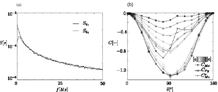
The first step consists in the characterization of the air flow in the test section with the coarse grid. In order to capture the low-frequency content of the turbulence, measurements of 20 minutes have been done and provide the spectra represented in Figure 4.

𝜌 = 690𝑘𝑔/𝑚³ 𝐿2,𝑎 = 0.02𝑚 𝐼𝑎= 0.38𝑘𝑔. 𝑚²

𝜌𝑎𝑖𝑟 = 1.25𝑘𝑔/𝑚³ 𝐿2,𝑏= 0.1𝑚 𝐼𝑏= 0.30𝑘𝑔. 𝑚²

𝐻 = 𝑒 = 0.042𝑚 𝐿2,𝑐= 0.2𝑚 𝐼𝑐 = 0.21𝑘𝑔. 𝑚²

𝐵 = 1𝑚 𝐿2,𝑑 = 0.3𝑚 𝐼𝑑= 0.15𝑘𝑔. 𝑚²

(a) (b)

Figure 4 - (a) Spectral density function of the turbulent components. (b) Moment, force and reduced moment coefficients for the 5 pivot positions (grey to black) and varying angle of attack.

RESULTS AND DISCUSSION

CONCLUSION

Acknowledgements

H. Vanvinckenroye was supported by the National Fund for Scientific Research of Belgium.

REFERENCES

[1] L. Christie, «craneaccidents.com,» 11 02 2012. [En ligne]. Available:

http://www.craneaccidents.com/2012/11/report/update/one57s-crane-problem/. [Accès le 15 02 2016].

[2] K. Mok, «Youtube.com. YouTube - Crane Spinning out of Control,» 2008. [En ligne]. Available: https://www.youtube.com/watch?v=0olg_j3289Q. [Accès le 15 02 2016].

[3] R. Ghigliazza et P. Holmes, «On the dynamics of cranes, or spherical,» International Journal of Non-Linear Mechanics, vol. 37, n° %17, pp. 1211-1221, 2002.

[4] Y. Sakawa et A. Nakazumi, «Modeling and Control of a Rotary Crane,» Journal of Dynamic Systems, Measurement, and Control, p. 107:200, 1985.

[5] J. Eden, A. Butler et J. Patient, «Wind tunnel tests on model crane structures,» Engineering Structures, vol. 5, pp. 289-298, 1983.

[6] J. Eden, A. Iny et A. Butler, «Cranes in storm winds,» Engineering Structures, vol. 3, pp. 175-180, 1981.

[7] Z. Sun, N. Hou et H. Xiang, «Safety and serviceability assessment for highrise tower crane to turbulent winds,» Frontiers of Architecture and Civil Engineering in China, vol. 3, pp. 18-24, 2009.

[8] D. Voisin, Etudes des effets du vent sur les grues à tour, PhD thesis éd., Ecole Polytechnique de l'Université de Nantes, 2003.

[9] D. Voisin, G. Grillaud, A. Beley-Sayettat, J. Berlaud et A. Miton, «Wind tunnel test method to study out-of-service tower crane behaviour in storm winds,» Journal of Wind Engineering and Industrial Aerodynamics, vol. 92, n° %17-8, pp. 687-697, 2004.

[10] H. Vanvinckenroye et V. Denoël, «Average first passage time of a quasi-Hamiltonian Mathieu oscillator with parametric and forcing excitations,» Journal of Sound and Vibration, 2017. [11] D. Yurchenko, A. Naess et P. Alevras, «Pendulum's rotational motion governed by a stochastic

Mathieu equation,» Probabilistic Engineering Mechanics, vol. 31, pp. 12-18, 2013.

[12] P. Alevras, D. Yurchenko et A. Naess, «Numerical investigation of the parametric pendulum under filtered random phase excitation,» 2013.

[13] N. Moshchuk, R. Ibrahim, R. Khasminskii et P. Chow, «Asymptotic expansion of ship capsizing in random sea waves - I. First-order approximation,» Int. J. Non-Linear Mechanics, vol. 30, n° %15, pp. 727-740, 1995a.

[14] F. Poulin et G. Flierl, «The stochastic Mathieu's equation,» Proceedings of the Royal Society A: Mathematical, Physical and Engineering Sciences, vol. 464, pp. 1885-1904, 2008.

[15] W. Garira et S. Bishop, «Rotating solutions of the parametrically excited pendulum,» Journal of Sound and Vibration, vol. 263, n° %11, pp. 233-239, 2003.

[16] M. Clifford et S. Bishop, «Approximating the Escape Zone for the Parametrically Excited Pendulum,» Journal of Sound and Vibration, vol. 172, n° %14, pp. 572-576, 1994.

[17] S. Bishop et M. Clifford, «Zones of chaotic behaviour in the parametrically excited pendulum,» Journal of Sound and Vibration, vol. 189, n° %11, pp. 142-147, 1996.

[18] X. Xu et M. Wiercigroch, «Approximate analytical solutions for oscillatory and rotational motion of a parametric pendulum,» Nonlinear Dynamics, vol. 47, n° %11-3, pp. 311-320, 2006.

[19] X. Xu, M. Wiercigroch et M. Cartmell, «Rotating orbits of a parametrically-excited pendulum,» Chaos, Solitons & Fractals, vol. 23, n° %15, pp. 1537-1548, 2005.

[20] K. Mallick et P. Marcq, «On the stochastic pendulum with Ornstein-Uhlenbeck noise,» Journal of Physics A: Mathematical and General, vol. 37, n° %117, p. 14, 2004.

[21] G. Chunbiao et X. Bohou, «First-passage-time of quasi-non-integrable-hamiltonian system,» Acta Mechanica Sinica, vol. 16, n° %12, pp. 183-192, 2000.

[22] W. Liu, W. Zhu et W. Xu, «Stochastic stability of quasi non-integrable Hamiltonian systems under parametric excitations of Gaussian and Poisson white noises,» Probabilistic Engineering

Mechanics, vol. 32, pp. 39-47, 2013.

[23] W. Li, L. Chan, N. Trisovic, A. Cvetjovic et J. Zhao, «First passage of stochastic fractinoal derivative systems with power-form restoring force.,» International Journal of Non-Linear Mechanics, vol. 71, pp. 83-88, 2015.

[24] T. Primozic, Estimating expected first passage times using multilevel Monte Carlo algorithm, University of Oxford, 2011.

[25] M. Gitterman, «Spring pendulum: Parametric excitation vs an external force,» Physica A: Statistical Mechanics and its Applications, vol. 389, n° %116, pp. 3101-3108, 2010a.

[26] N. Moshchuk, R. Khasminskii, R. Ibrahim et P. Chow, «Asymptotic expansion of ship capsizing in random sea waves - II. Second-order approximation,» Int. J. Non-Linear Mechanics, vol. 30, n° %15, pp. 741-757, 1995b.

[27] J. Hamalainen, J. Virkkunen, L. Baharova et A. Marttinen, «Optimal path planning for a trolley crane: fast and smooth transfer of load,» IEEE Proceedings - Control Theory and Applications, vol. 142, pp. 51-57, 1995.

[28] V. Denoël et E. Detournay, «Multiple scales solution for a beam with a small bending stiffness,» Journal of Engineering Mechanics, vol. 136, n° %11, pp. 69-77, 2010.

[29] Z. Schuss, Theory and Applications of Stochastic Processes - An analytical approach, Applied Mathematical sciences éd., vol. 170, New-York: Springer, 2010, pp. 81-110.

[31] H. Vanvinckenroye et V. Denoël, «Stochastic rotational stability of tower cranes under gusty winds,» chez Proceedings of the Sixth International Conference on Structural Engineering, Mechanics and Computation, 2016.

[32] H. Vanvinckenroye, «Monte Carlo simulations of autorotative dynamics of a simple tower crane model,» 2015.