F
ACULTYO
FA
PPLIEDS
CIENCESAEROSPACE AND MECHANICAL ENGINEERING DEPARTMENT THERMODYNAMICS LABORATORY
S
TUDY
, M
ODELLING
A
ND
A
NALYSIS
O
F
H
EAT
P
UMPING
S
OLUTIONS
I
N
A C
OMMERCIAL
B
UILDING
Stéphane Bertagnolio
Thesis Submitted in Partial Fulfilment of the Requirements for the Degree of
ACKNOWLEDGEMENTS
I am grateful to Professor J.Lebrun who oversaw this work and enabled me to follow this great project. I thank him for his trust and supervision.
I also thank Jules Hannay and Cleide Aparecida Silva for their suggestions and their help.
Special thank to Bernard Georges for his permanent availability to reply to any question, and to Vincent Lemort for his advises. I also thank Philippe Ngendakumana, Philippe André and Georges Heyen for their corrections.
A great thank to Pierre Gustin, Sylvain Quoilin, Laurie Detroux and Ludovic Buckinx for their support, their friendship and the great environment of work.
Lastly, I want to thank all the people who were a real support for me during the five last years.
This work is carried out in the frame of the IEA-ECBCS (International Energy Agency – Energy Conservation in Buildings and Community Systems) Annex48: “Heat Pumping and Reversible Air Conditioning”. The aim of this work is to study the possibility of integration of a reversible heat pumping system into the existing HVAC system of a “commercial” building (which includes laboratories).
A pre-audit of the actual HVAC installation is carried out and presented. Numerical models of the building and of the coupled HVAC installation are developed and implemented on EES (Engineering Equation Solver, ©F-Chart Software) to run yearly simulations. The main retrofit opportunity is the use of reversible heat pumping, with the extracted air as heat source, to heat the building. Other retrofit possibilities, as “change over” technique or cool thermal energy storage, are also modelled, simulated and analysed. The environmental and economical aspects of each retrofit opportunity are approached.
The reversible heat pumping coupled with a change over technique is generally able to satisfy the heating demand of the building. However some interventions of the existing natural gas condensing boilers, as back boosting devices, are sometimes necessary during winter. The economical and environmental studies reveal a quite short payback time and a significant reduction of CO2 emissions. The advantages of the cool thermal storage solution are not obvious and have not been highlighted in the present case.
Ce travail est réalisé dans le cadre du projet IEA-ECBCS (International Energy Agency – Energy Conservation in Buildings and Community Systems) Annex48 : « Heat Pumping and Reversible Air Conditioning ». Le but de ce travail est l’étude de la possibilité d’intégration d’un système de pompe à chaleur réversible dans l’actuelle installation de conditionnement d’air d’un bâtiment commercial comprenant des laboratoires.
Un pre-audit de l’actuelle installation est réalisé et présenté. Plusieurs modèles numériques du bâtiment et de l’installation HVAC sont développés et compilés au moyen du programme EES (Engineering Equation Solver, ©F-Chart Software) en vue de réaliser une simulation annuelle. La principale possibilité de modification de l’installation actuelle est l’utilisation d’un système de pompe à chaleur réversible, utilisant l’air extrait comme source de chaleur, pour répondre à la demande de chaud du bâtiment. D’autres opportunités, comme l’utilisation d’une technique de « change over » ou d’un système de stockage de froid, sont aussi modélisées, simulées et analysées. Les aspects environnementaux et économiques sont également abordés.
L’utilisation d’un système de pompe à chaleur, couplé à une technique de « change over », est, en général, capable de satisfaire la demande de chaud du bâtiment. Toutefois, l’intervention des chaudières au gaz naturel, comme dispositif de chauffage auxiliaire, est parfois nécessaire pendant la période hivernale. Les études économiques et environnementales donnent un temps de retour sur investissement relativement court et une réduction significative des émissions de CO2. Les avantages du système de stockage de froid ne sont pas évidents et n’ont pas pu être mis en avant dans le cas présent.
PART I : DESCRIPTION & PRE-AUDIT OF THE EXISTING SYSTEM... 2
I.1. BUILDING... 3
I.1.1. Dividing the building in zones ... 3
I.1.2. Orientations and exposure ... 4
I.1.3. Building thermal characteristics... 5
I.2. AIR CONDITIONING SYSTEM... 6
I.2.1. Offices Floor ... 6
I.2.2. Laboratories Floor... 8
I.2.3. Fourth & Fifth Zone... 9
I.3. REFRIGERATION & HEATING PLANT... 10
I.3.1. Heat Production... 10
I.3.2. Cold Production... 10
I.4. WATER DISTRIBUTION NETWORK... 11
I.5. PRE-AUDIT OF THE INSTALLATION... 13
I.5.1. Electricity & Gas Consumptions ... 13
I.5.2. Thermal Signature ... 17
I.6. CONCLUSIONS... 19
I.7. RETROFIT OPPORTUNITIES... 20
PART II : MODELLING OF THE INSTALLATION... 22
II.1. AIM & PHILOSOPHY OF THE MODELLING PHASE... 23
II.2. BUILDING MODEL... 24
II.2.1. Zone Sensible Heat Balance ... 25
II.2.2. Structure Energy Balance... 25
II.2.3. Fabric Heat Transmission ... 26
II.2.4. Ventilation Enthalpy Flow rate ... 27
II.2.5. Sensible Heat Gains... 27
II.2.6. Zone Water Balance ... 29
II.2.7. Building Model Parameters... 30
II.3. HVAC SYSTEM MODEL... 32
II.3.1. Air Handling Unit Model... 32
II.3.1.1. Heating Coil Model ... 33
II.3.1.2. Cooling Coil Model ... 36
II.3.1.3. Recovery Loop Model ... 41
II.3.1.4. Steam Humidifier Model ... 44
II.3.1.5. Fan Model... 45
II.3.1.6. Duct Model ... 45
II.3.1.7. Air Handling Unit Global Model Parameters... 46
II.3.2. Terminal Unit Model ... 47
II.3.3. Cooling Plant Model ... 48
II.4.3. Control Laws ... 54
II.4.3.1. Offices ... 54
II.4.3.2. Laboratories ... 56
II.5. OUTPUTS OF THE MODEL... 56
PART III : SIMULATION RESULTS AND ANALYSIS... 57
III.1. INTRODUCTION... 58
III.2. PRESENT SITUATION – SIMULATION RESULTS... 58
III.2.1. Temperature Profiles... 58
III.2.1.1. Laboratories... 58
III.2.1.2. Offices ... 60
III.2.1.3. Air Handling Units ... 62
III.2.2. Heating & Cooling Power Demands ... 63
III.2.2.1. Laboratories... 63
III.2.2.2. Offices ... 64
III.2.2.3. Global demands... 64
III.2.3. Electricity & Gas Consumptions... 65
III.3. CONCLUSIONS... 67
PART IV : RETROFIT & IMPROVEMENT OPPORTUNITIES... 68
IV.1. PLANT MODIFICATION... 69
IV.1.1. Recovery Strategy ... 69
IV.1.2. Reversible Heat Pumping ... 69
IV.1.3. Change Over Technique & Re-starting ... 71
IV.1.4. Thermal Energy Storage... 73
IV.2. MODELLING & CONTROL... 75
IV.2.1. Heat Pump Model... 75
IV.2.2. Heat Source Model ... 76
IV.2.3. Change Over Modelling ... 77
IV.2.3.1. Parallel Assembly ... 78
IV.2.3.2. Series Assembly ... 79
IV.2.3.3. Choice and globalisation work... 81
IV.2.4. New Re-starting Strategy... 83
IV.2.5. Thermal Energy Storage Model ... 83
IV.2.6. Control Strategy ... 85
PART V : MODIFIED PLANT - SIMULATION RESULTS... 87
V.1. INTRODUCTION... 88
V.2. SIMULATION RESULTS... 89
V.2.1. System n°1 – Actual Installation... 89
V.2.2. System n°2 – Recovery Strategy... 90
V.2.2.1. Temperature & Power Profiles... 90
V.2.2.2. Economical Aspect & Conclusion ... 92
V.2.3. System n°3 – Heat Pumping... 94
V.2.3.1. Temperature Profiles ... 94
V.2.3.2. Conclusion... 97
V.2.4. System n°4 – Heat Pumping & Installation Adaptation ... 98
V.2.4.1. Temperature Profiles ... 98
V.2.5. System n°5 – Thermal Energy Storage ... 104
V.2.5.1. Power Profiles ... 105
V.2.5.2. Consumptions ... 107
V.2.5.3. Conclusion... 108
V.4. ECONOMICAL ASPECT... 109
V.4.1. Initial Investment and costs definition ... 109
V.4.2. Evaluation Methods ... 109
V.4.2.1. Payback Time Method... 109
V.4.2.2. Net Present Value Method ... 110
V.4.2.3. Internal Rate of Return Method... 110
V.4.3. Economic Evaluation of System n°4 ... 111
V.4.4. Economic Evaluation of System n°5 ... 112
V.4.5. Conclusion ... 113
V.5. ENVIRONMENTAL ASPECT... 114
V.6. CONCLUSIONS... 116
CONCLUSION... 117
INTRODUCTION
In 2006, the IEA ECBCS executive committee decided to launch the three-year work phase of the Annex48 on “Heat Pumping and Reversible Air Conditioning”. This work is made in the frame of this project and concerns the first Belgian case study.
Substituting a heat pump to a boiler may save more than 50% of primary energy, if electricity is produced by a modern gas-steam power plant (even more if a part of that electricity is produced from a renewable source). “Heat pumping” is probably today one of the quickest and safest solutions to save energy and to reduce CO2 emissions
Most of air-conditioned commercial buildings offer attractive retrofit opportunities, because: 1) When a chiller is used, the condenser heat can cover (at least a part of) the heating
demand (condenser heat recovery method);
2) When a chiller is not (fully) used for cooling, it can be (at least partially) re-converted into heat pump (reversible heat pumping method).
Nowadays, the retrofit work of an existing building should take all possibilities of heat pumping into consideration, in such a way to make air conditioning as “reversible” as possible.
In the present work, a detailed study of the first Belgian case study is realized. First, a description of the building and a pre-audit of the HVAC installation is presented. This phase is useful to determine the main retrofit and improvement opportunities.
The second part of the report concerns the modelling phase of the work. Several numerical models are developed and implemented on EES (Engineering Equation Solver, © F-Chart Software). First, the building is divided in zones and each zone is modelled using a dynamic mono-zone building model. This first model is coupled to a complete HVAC system model, based on independent reference and simplified models.
The third part of this report presents the first results obtained, thanks to the simulations of the actual installation, with previously presented models. The computed values of the consumptions are compared with the measured consumptions.
The fourth part concerns the explanation of the main retrofit opportunities which are envisaged. Practical information and models are be presented in this chapter.
In the fifth part, the results related to the studied retrofit opportunities are shown, detailed and compared. Economical and environmental evaluations of these possible improvements is presented.
I.1. Building
I.1.1. Dividing the building in zones
The case study building considered in the present report is a laboratory building erected in 2003 in the region of Liège (Belgium). To allow an easier understanding of the layout of the building, we can divide it in five distinct zones (Figure I-1).
The first considered zone (noted “zone I”) corresponds to the offices (2nd floor, about 1602 m²). This zone is totally surrounded by classical double-glazing on its entire perimeter. The frontages are partially shadowed by the cornice of the roof. The offices are disposed on the perimeter of the zone, in the centre, three small meeting rooms and one copy room are closed using very light walls (as light panels and simple glazing).
The second zone (“zone II”) corresponds to the technical room, where all the air handling units (AHU), chillers, boilers, pipes and air ducts are installed (about 1852 m² with the stair-well). The frontages of this stage are totally opaque and insulated from the outside (concrete and insulated wall covered with aluminium facing). This zone is characterized by a quite constant and high temperature (generally oscillating between 21-24 °C).
The third zone (“zone III”, on ground floor) contains the laboratories of the building. In fact, the laboratories’ stage includes two main zones: one large opened laboratory and a smaller insulated and slightly pressurized laboratory zone. In the frame of this work, we will consider these two “sub-zones” as a large one. The laboratory is glazed on its two lengths of frontage and totally closed on its width (concrete walls and aluminium facing). The last side of the zone is the limit between zones III and IV. Supposing that zones III and IV have close temperatures (which is really close to the reality), we can neglect the heat transfer between the two zones.
The fourth zone (zone IV) corresponds to several sanitary facilities (showers, bathrooms…etc), cloakrooms dedicated to the laboratory’s employees and the main stairwell of the building (about 585 m²). The external frontages of this zone are totally closed and opaque (concrete wall and aluminium facing).
The fifth zone (zone V) regroups the “logistic” rooms as cold rooms, warehouse and storeroom (about 585 m²) and is closed on its perimeter by concrete walls and a large door. An open parking space is allowed to the employees under the laboratory zone (zone III). The whole building counts another smaller part which includes three meeting rooms, one dining room and a cellar disposed on three stages. This appendix is connected to the main building by the reception hall.
I.1.2. Orientations and exposure
As it is shown on Figure I-3, the large frontages of the building are oriented North and South. Figure I-2 shows the south frontage of the building.
Figure I - 2 : South Frontage
W E
I.1.3. Building thermal characteristics
The thermal characteristics of the building’s envelope can be described in a simplified way by distinguishing two components only (Aparecida Silva et al., 2007) “classical double glazing” (U=2.8 W/K.m²) and “opaque surface” (U=0.8 W/K.m²).
U values, windows and opaque surfaces areas and UA values (heat transfer coefficients) in [W/K], are given, for the entire building, in Table I-1. It is obvious than only the external surfaces are considered in the following calculation.
Double glazing windows
Roof Ground/floor Opaque
external walls Total UA U (W/Km²) 2.8 0.8 0.8 0.8 A (m²) 926.2 1853 1853 1248 UA (W/K) 2593 1482 1482 998 6555
Table I - 1 : Envelope Heat Transfer Coefficients
So, we can assume that the heat transfer coefficient of transmission trough building envelope is about : 6555 W/K.
The global UA values of the external surfaces of the five zones are presented in Table I-2:
Zone I Zone II Zone III Zone IV Zone V A (m²)
Double glazing windows 549 0 377 0 0 A (m²) Roof 1602 250 (0) (0) (0) A (m²) Ground/floor (0) (0) 1268 (0) 585 A (m²) Opaque walls 0 664 57 230 297 UA (W/K) 2820 731 2115 184 705
I.2. Air Conditioning System
I.2.1. Offices Floor
The 2nd floor (offices zone) is ventilated with 100% fresh air at a flow-rate of 5050 m³/h for the entire zone. An air handling unit, called GP4/GE4 (for Pulsing Group and Extraction Group n°4) ensures partially the follow-up of the temperature set point of the zone.
This Air Handling Unit includes filters, one glycol-water recovery loop placed between fresh and vitiated air, one heating coil, one cooling coil and fans (Figure I-4). The recovery loop is composed of two water/air coils disposed on supply and exhaust ducts and a glycol-water loop. The exhaust side coil works in “cooling regime” and recovers sensible (and latent, in some conditions) heat by decreasing the air temperature (and its water content). The recovered heat is transmitted to the supply side coil using the glycol-water loop. This second coil works in “heating regime” and increases the supply air temperature. Actually, this recovery system is not regulated and works at full glycol flow rate during AHU functioning periods. The cooling coil is supplied with chilled water coming from the chilled water network at a temperature of about 7-8°C. The heating coil installed in this AHU is supplied with hot water coming from the hot water network at a temperature of about 70-80°C. Whereas the heating and cooling coils are regulated using, respectively, temperature and flow rate control, the recovery loop is not regulated and works at maximal water flow rate all the year long.
Fresh supplied, filtered, preheated or cooled (but not humidified) air is diffused in the rooms
In small rooms, like offices, supplied air is diffused only trough the terminal units at a flow rate of about 60 m³/h and extracted by an unique extraction orifice at a flow rate of 60m³/h. Larger rooms, like small meeting rooms, are fed in fresh air trough the terminal unit and trough additional air supply diffusers. The global extraction of vitiated air is made at a flow rate of 3800 m³/h for the entire zone. The overpressure in the zone prevents any air infiltration.
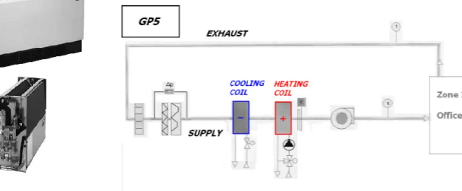
An additional AHU, called GP5, works in closed loop (with 100% recirculated air) and ensures the conditioning of the large central open space. This group works at a flow rate of about 5000 m³/h and includes a filter, a heating coil, a cooling coil and a fan.
The control strategy is similar to the other AHU (GP/GE4) and is charged to maintain the set-point temperature in the zone.
Several types of terminal units are installed. Each device has five different working speeds (characterized by 5 different air flow rates) but are similar in their structure (As built File, 2003). Installed Terminal Units (TU) characteristics are presented in Table I-3
Terminal Unit model TU size 3 TU size 5 TU size 6 Type Cooling&Heating 4 pipes Cooling&Heating 4 pipes Cooling&Heating 4 pipes number 40 6 2
location offices Meeting rooms Meeting rooms
Air flow rates (m³/h) 180-280-410-575-750 210-320-465-670-960 210-325-475-675-975 Heating Power (kW) 1.9-2.6-3.4-4.1-4.6 2.3-3.1-4.0-5.0-6.0 2.4-3.4-4.4-5.5-6.7
Cooling Power (kW) 1.5-2.1-2.7-3.3-3.9 1.5-2.2-3.0-3.7-4.5 1.9-2.7-3.6-4.5-5.7 Table I – 3 : Terminal Units Characteristics
Heating and cooling powers are given in nominal conditions but correction factors are also given by the manufacturer to allow the calculation of actual heating and cooling powers, as function of working conditions.
The offices are occupied by about 70 people between 8:00 and 17:00, five days per week. The zone is ventilated using the air handling unit between 6:00 and 20:00 five days per week too. Terminal units ensure the set point temperature follow-up during the same period but are used for a “re-starting” on Sunday evening between 15:00 and 20:00.
The first floor (technical room) is occupied only by a little maintenance team between 8:00 and 17:00 and is not conditioned. The high and constant temperature of the zone is only due to the heat loss of the different components of the HVAC installation (Air Handling Units, ducts, pipes…etc).
I.2.2. Laboratories Floor
The ground floor (laboratories) is ventilated with 100% fresh air at a flow rate of about 33000 m³/h for the entire zone. The extraction is characterized by the same air flow rate. Three independent AHUs, called GP/GE 1,2 & 3, ensure completely the conditioning and the follow-up of temperature set point in the zone (approximately 23°C). Two groups of 11500 m³/h (GP/GE 2 & 3) are equipped with steam humidifiers controlled to maintain a relative humidity set point of about 50% and are in charge of the large part of the zone. One smaller group (GP/GE 1) of about 10000 m³/h takes care of the smaller pressurized part of the laboratories. The other components of these three AHUs are similar to those which compose the AHU “GP/GE4” (see Figure I-7).
Hygienic considerations could justify the use of electrically heated self-contained steam humidifiers, fed with normal tap water. Indeed, reached high temperatures and absence of stagnant water prevent any risk of bacterial contamination, which could be critical for laboratory’s processes.
Supplied air is directly brought trough some textile cylindrical porous diffusers which are suspended in the zone (Figure I-8). The comfort conditions (approximately, 23°C/50%) are maintained only using the three AHUs, there is no other air conditioning system in the zone.
Ventilation and air conditioning of the zone is ensured 24h per day, 7 days per week all the year. About 60 people work in the laboratories during day (between 8:00 and 17:00) and, in addition to these 60 employees, about 6 people are present in the zone 24h/24.
Whereas, in the offices zone, the internal sensible gains are classical offices gains, in the laboratories, internal sensible gains are higher because of all the apparatuses installed in the zone. Numerical values will be discussed later.
A smaller AHU (called GP/GE7) is in charge of a little closed room installed in the laboratories. This zone is a “humidity-controlled” room and is characterized by the following set points : 23°C/65-70%. Considering that this room is of reduced size comparing to the entire zone and that the corresponding ventilation rate is low, its presence will be neglected in the following calculations.
I.2.3. Fourth & Fifth Zone
The fourth zone (sanitary facilities and cloakrooms) is not conditioned but is only heated using classical water radiators. This room has not a particular occupancy profile and is maintained at a temperature near 23°C.
The fifth zone (warehouse and storage) is conditioned using several cooling and heating terminal units. As it was the case for the fourth zone, this room has not a particular occupancy profile. Four cold rooms are installed in this zone. Two negative (-20°C) and two positive cold rooms (4°C) are equipped with air condenser.
The appendix building is conditioned thanks to an additional AHU, called GP/GE 6, working at an airflow rate of about 1600 m³/h. This group is similar to the others previously presented and diffuse the treated air trough pulsing plenum (hidden in the corners of the rooms) and ceiling cassettes air conditioners. These conditioning units work like classical terminal units and are supplied with hot and chilled water coming from hot and chilled water networks.
I.3. Refrigeration & Heating Plant
The installed power plant is composed of two recent condensing boilers and one air-cooled chiller. Theses elements are installed in the central equipment room of the building (1st floor).
I.3.1. Heat Production
The heat production is ensured by two high efficiency gas condensing boilers of 300 kW each (Figure I-9). These boilers supply the hot water network with water at a temperature of about 70-80°C and an efficiency of about 90% (based on HHV) in full load conditions. Of course, at this temperature regime, the boilers do not function in condensing mode.
I.3.2. Cold Production
An air condenser chiller (Figure I-10) ensures the production of chilled water at a temperature of 7-8°C for the whole building. The chilled water is used to supply the different cooling coils of the HVAC system (AHU’s cooling coils and TU’s cooling coils).
This chiller is characterized by a nominal (12/7°C entering/leaving evaporator temperatures; 35°c ambient temperature) cooling capacity of about 399,1 kW. The corresponding power demand (compressors only) is about 139,3 kW. The cooling of the condenser is ensured by
Figure I – 9 : Gas Condensing Boiler
I.4. Water Distribution Network
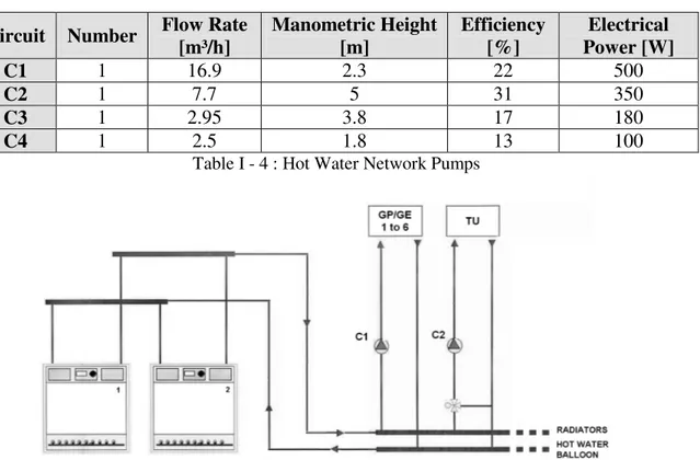
As it has been said, hot water production is ensured by two condensing boilers disposed in parallel. Four main pumps ensure the circulation of the hot water in the hot water network (Table I-4). The first pump (C1) fed the heating coils of the air handling units and the second (C2), the heating coils of the terminal units. The third pump (C3) ensures the supplying of radiators. The fourth pump ensures the circulation in the (sanitary) hot water tank. The third pump is not taken into account in our calculation because the radiators that they supply are not in the modelled zones (but in zone IV). Not knowing the rate of demand for sanitary hot water, hot water tank and its pump are not integrated in the calculations. So, only the pumps C1 and C2 will be taken into account in the calculations. A simplified scheme of the hot water networks is presented in Figure I-11.
Circuit Number Flow Rate [m³/h] Manometric Height [m] Efficiency [%] Electrical Power [W] C1 1 16.9 2.3 22 500 C2 1 7.7 5 31 350 C3 1 2.95 3.8 17 180 C4 1 2.5 1.8 13 100
Table I - 4 : Hot Water Network Pumps
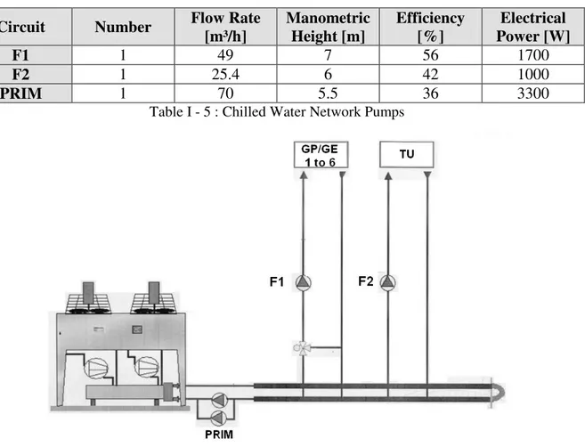
Three pumps are used for the distribution of chilled water (Table I-5). The first pump (F1) fed the cooling coils of the air handling units and the second (F2), the cooling coils of the terminal units. The third pump (PRIM) is in charge of the primary chilled water network and ensures the water circulation in the evaporator. These pumps are not equipped with inverters, so, we can suppose that they work in nominal conditions as soon as there is a cooling demand in the building. Vanes ensure regulation of the chilled water network.
A simplified scheme of the hot water networks is presented in Figure I-12 .
Circuit Number Flow Rate [m³/h] Manometric Height [m] Efficiency [%] Electrical Power [W] F1 1 49 7 56 1700 F2 1 25.4 6 42 1000 PRIM 1 70 5.5 36 3300
Table I - 5 : Chilled Water Network Pumps
I.5. Pre-audit of the Installation
I.5.1. Electricity & Gas Consumptions
The audit of an existing HVAC system consists in analysing the available information about actual energy consumptions and global performances. In the following pre-audit, only directly available information (visual verifications, as-built records analysis, operating costs and consumptions, short and limited measurements) and very simple calculation will be used to analyse the installation and identify the most attractive retrofit opportunities (Lebrun et al., 2006a; Aparecida Silva et al.,2007).
After having regarded the building’s design and the HVAC system’s functioning, it’s time to consider the available data as electrical and gas consumptions. As usually, monthly records of electricity and gas energy consumptions are available. The electrical consumption between January 2005 and July 2006 is plotted in Figure I-13. It appears that the average electricity consumption for this period is floating around 130000 kWh/month. It seems difficult to highlight a possible seasonal effect but the effect of steam humidification can be noted. Indeed, winter month’s consumptions are greater than summer month’s consumptions. This observation can be explained by the fact that (winter) steam humidification is more consuming than (summer) cooling and will be better highlighted in the following figures.
The conclusions are different for the measured gas consumptions (Figure I-14) for the same period. Indeed, variations are much larger and show the seasonal effect (low consumptions during summer months and high consumption during winter months).
Using this data, it is possible to evaluate the monthly averages electrical powers (Figure I-15). Obviously, it is also impossible to highlight a possible seasonal effect. However, it is again possible to highlight the effect of steam humidification on electrical power demand. Indeed, electrical power demand peaks due to steam humidification seem to be greater than those due to the chiller consumption. On the whole year, averages, day, night and global electrical powers are, respectively, 205.5, 146.5 and 172.1 kW.
On Figure I-16, monthly averages electrical powers are plotted as function of the outdoor temperature. The identified linear regression has a negative slope which illustrates an already made observation : steam humidifier consumption during winter months is higher than chiller consumption during summer months. In pink, the estimated humidification consumption is plotted and seems to reach about 120kW at 0°C. In green, the “constant” power demand (lights, appliances, fans and pumps) is plotted. For the entire building, this power reaches about 80 kW.
The isolated point corresponds to December 2005. The low electrical demand is due to the fact that, during this a part of the month, the laboratories are closed and the employees are on holidays. Usually, this period is used for the maintenance of the HVAC installation.
Considering the hypothesis made on the humidification consumption, a part of the summer electrical power demand (about 80 kW) cannot be explained by the humidifiers but, partially, by the chiller consumption. However, if the humidifiers consumption was null at this outdoor temperature (16°C), the electrical power demand curve would have a “U” shape and would increase at high outdoor temperature. Actually, this is not the case and this summer consumption cannot be explained.
A measure campaign is currently envisaged and should begin soon.
Winter months & Summer
Figure I-17 shows the measured electrical power demand due to the coldrooms chillers. Two average values can be computed : a “week average value” corresponding to the occupancy periods during which the coldrooms are opened a few times per day and a “weekend average value” during which the coldrooms stay closed all the time.
I.5.2. Thermal Signature
In the frame of an auditing project, the thermal signature is the distribution of the fuel/gas power defined in monthly average (between January 2005 and July 2006 in our case), as function of the external dry bulb temperature (Lebrun et al., 2006a; Aparecida Silva et al.,2007). Figure I-18 gives this thermal signature for the concerned building. It gives a good correlation factor (0.94) and allows a meaningful linear regression to be identified. Its equation is given on Figure I-18. The slope of this law (-14.05 kW/K) should correspond to the global average heat transfer coefficient of the building.
Using the building thermal characteristics and the building envelope’s heat transfer coefficient (UA = K = 6.555 [kW/K]), it is possible to retrieve the “average heat transfer coefficient” given by thermal signature correlation (Aparecida Silva et al., 2007).
Considering a ventilation air flow rate of about 38000 m³/h for the whole building (10000 m³/h for GP1, 11500 m³/h for GP2 & GP3 and about 5000 m³/h for GP5, see HVAC system description), the mechanical ventilation heat transfer coefficient (or thermal capacity flow rate) is calculated as follows :
The calculation gives :
Considering that, in nominal conditions, recovery loops have an efficiency of about 42% (given in manufacturer data), we can compute the “heat recovery potential” :
This means that the net ventilation heating demand is about : 12.73 – 5.7 = 7.03 kW/K
The global heating demand of the building can be estimated by adding transmission (trough building’s envelope) and ventilation terms :
Then, the total heating demand heat transfer coefficient is about : 13.585 [kW/K]. Note that this value has not been modified to take ventilation intermittency into account. Indeed, the greatest part of the total ventilation flow rate (39600 m³/h) is due to the ventilation of the laboratories (33000 m³/h, 24h/day, 7d/week).
The value obtained thanks to this rough calculation is in fair agreement with the slope (14.05
[kW/K]) of the building “thermal signature” as shown in Figure I-18. This result is very
important and allows us to affirm that the gas consumption can be explained by the building’s heating demand. Moreover, these results are encouraging and confirm the hypotheses made on the heat transfer coefficients.
I.6. Conclusions
In spite of recent character of the installation and its potential high efficiency, gas and electrical consumptions are important and the source of high costs (and CO2 emissions). An important part of these costs is due to the steam humidification systems. Indeed, these apparatuses are very hygienic and characterized by their simplicity and facility of use but are also great consumer of electrical energy. However, in the case of laboratories, the use of steam humidification instead of adiabatic humidification can be justified. A first proposal could be to verify if the needs for humidification and these high temperature and humidity set points (23°C/50%) are justified.
Whereas the winter electrical consumption is quite well explained (by constant consumptions and steam humidifiers consumptions), at the moment, it is not possible to affirm that the summer electrical consumption is totally due to the chiller. The modelling of the installation will be useful to clear up this specific point.
As the thermal signature shown it, the gas consumption can be explained by the heating demand of the building. Indeed, the thermal signature coefficient corresponds to the heat transfer coefficient of the building’s envelope.
I.7. Retrofit Opportunities
Nowadays, the Air Handling Units which are connected to the laboratories are functioning 24 hours per day in full fresh air mode and are already equipped with heat recovery loops recovering approximately 40% of available sensible heat. The remaining sensible (and latent!) heat is (are) still available and recoverable. An interesting improvement would be the use of a heat pump to recover this wasted energy. The extracted air, at the exhaust of the recovery coils, could be used as heat source for heat pumping and the produced heat as hot source for building’s heating. A possible arrangement is suggested in Figure I-19. The actual air-cooled condenser chiller would be replaced by a water-cooled one which could be used in chiller and in heat pump mode. Supplementary air-water coils would be added in the extracted air duct of the main Air Handling Units (GE 1,2&3, functioning at constant air flow rate 24/24), downstream of the existing heat recovery coil, to recover the available heat and supply the heat pump evaporator. On the condenser side, the produced low temperature hot water (about 55°C at condenser exhaust) could be used to supply heating devices, as AHU heating coils or TU heating coils. In the case of a lack of heat transfer surface (due to the use of low temperature hot water instead high temperature hot water produced by boilers), cooling coils could be used as secondary heating coils (using a “change over” technique).
In addition to this main retrofit opportunity, several adaptations could also be brought to the actual installation :
- To program a recovery strategy to avoid the waste occurring when recovery loop and cooling coil are working simultaneously,
- To study the possibility of a decreasing of the ventilation flow rate and of the indoor conditions (temperature and humidity) during unoccupied periods,
- To imagine and envisage other (clean and secure) humidification systems.
A part of these proposals will be investigated, studied and detailed in the following. However, the two last opportunities (modification of the ventilation rate and humidification system) will
laboratories) are the zones in charge of the main part of the consumptions due to the HVAC system. On one hand, laboratories and offices are characterized by an important HVAC system, composed of large air handling units and a high number of terminal units. On the other hand, the remaining zones are equipped with only some radiators (about 6) and a small air handling unit (GP/GE 6). Moreover, the whole building is ventilated (with full fresh air) at a rate of about 39600 m³/h when zones I and III totalise 38000 m³/h. All theses observations justify the fact that, in the following work, only zones I and III will be taken into account. The other zones will be studied later, in the frame of the IEA Annex48 project. Of course, only the equipments corresponding to the studied zones will be taken into account in the calculations.
II.1. Aim & Philosophy of The Modelling Phase
While, in a pre-audit procedure, the identification of the building heating & cooling demands is not envisaged (heat/cool counters are not often installed in buildings), the calculation of theoretical demands and corresponding energy consumptions appears logically at the start of a feasibility calculation and detailed study of retrofit opportunities.
Considering the number of parameters and influences which are involved in this type of calculation, it seems rational to run simulation model rather than very global and hypothetical weather indexes (similar to heating degree-days). For this targeted work, simulation models are required that are sufficiently reliable, accurate and robust.
The level of detail required for each calculation can be very different. For heating calculations, the major issues are a correct description of the building envelope and an accurate evaluation of the air renewal. For cooling calculations, the fenestration area and orientation, the level and distribution of the internal gains, the ventilation rates, and the geographical location appear as critical issues. Most of these issues are explicitly taken into account in the developed models.
The presented model could be divided in two main parts : - a dynamic building model,
- a static HVAC system model.
The first part of the global model ensures the calculation of the heating and cooling loads whereas the second part (HVAC system model) involves moving from building demands to system energy consumptions.
In both situations, the issue is to define the optimal level of detail of the model in relationship to the amount of information collected during the pre-auditing phase and the required qualities of the model. To this end, only one building model will be used in the following work but three types of models will be developed for the HVAC system components:
- complete, validated, detailed and accurate models (called “mother models”), used to compute components characteristics and properties (basing on manufacturer data) - simplified, robust and more easy-to-use models (called “daughter models”), using the
previously defined characteristics to run simulations,
- Simplified, robust and easy to tune models (called “orphan models”), directly tuned using manufacturer data.
Most of these models have already been developed, validated and used in University of Liège (André et al., 2006a; André et al., 2006b) in the frame of the following research projects :
- IEA ECBCS Annex 10 - ASHRAE Primary Toolkit - IEA ECBCS Annex 40 - IEA ECBCS Annex 43 - AUDITAC
II.2. Building Model
The following building model has been developed as a “benchmarking – auditing” tool in University of Liège (André, Lebrun et al., 2006a) and implemented on “EES” (Engineering Equation Software, © F-Chart Software).
Obviously, the simulation model includes realistic and physical considerations, as : - building (static and dynamic) behaviour,
- weather and occupancy loads, - solar exposure and orientations,
- characteristics of materials composing the building’s envelope.
The presented building model is based on a very simplified equivalent R-C network (with only two thermal masses, Figure II-1), corresponding to a mono-zone open plan floor with light internal “curtain” walls and external glazed walls. This scheme corresponds to a typical office building, mainly composed of a lattice concrete structure and light glazed walls.
A sensible heat balance is established on the indoor node which is connected to the structure (first thermal capacitance, right branch), to the outside environment (left branch) and to the ventilation system (top branch). Terminal Units and several other “injectors” (as solar, occupancy, lighting and appliances gains) are taken into account and called “Sensible Heat Gains”. The energy storage effect inside the zone (air, walls and furniture) is represented by the second thermal capacitance (bottom branch).
II.2.1. Zone Sensible Heat Balance
The equations corresponding to this first sensible heat balance and the calculation of the energy storage inside the indoor environment are presented below :
where ta,in is the indoor temperature (at time = t), in °C, ta,in,1 is the initial indoor temperature (at t = 0), in °C, Cin is the inside thermal capacity, in J/K,
The inside thermal mass, used in equation (II.2.2), is computed using the following formula :
where Vin is the internal volume of the zone, in m³ ρa is the air density, in kg/m³
cp,a is the air specific heat, in J/kg-K
The air capacitance is corrected by a hypothetical factor, supposed to take into account the capacity of all the internal surfaces and equipments (walls and furniture). The authors propose a value of about 5 for this correction factor (Lebrun, 2006b).
II.2.2. Structure Energy Balance
The structure contribution is computed using the following balance :
The first term of equation (II.2.4) is the heat flow coming from the internal structure and is computed as follows : (II.2.1) (II.2.2) (II.2.3) (II.2.4) (II.2.5) (II.2.6)
where Rstruct is the thermal resistance corresponding to the global exchange (convective and radiative) between the ambiance and the structure, in K/W,
tstruct is the structure temperature (at time = t), in °C, Afloor is the floor surface, in m²,
hin is the inside global exchange coefficient, in W/m²-K.
The second term appearing in equation (II.2.4) is the energy stored in the structure :
where Cstruct is the structure thermal capacity, in J/K,
tstruct,1 is the initial structure temperature (at t = 0), in °C, efloor is the floor thickness, in m,
rhofloor is the floor density, in kg/m³, cfloor is the floor specific heat, in J/kg-K.
II.2.3. Fabric Heat Transmission
The heat flow passing trough the external envelope of the zone is given by a global heat transfer coefficient (AUfrontages) multiplied by the indoor-outdoor temperature difference, at time t.
where tout is the outdoor dry temperature, in °C, Awindows is the glazed walls surface, in m², Aopaque,frontages is the opaque walls surface, in m²,
Uwindows is the double-glazing conductive heat transfer coefficient, in W/m², Uopaque,frontages is the opaque walls conductive heat transfer coefficient, in W/m².
(II.2.7)
(II.2.8)
II.2.4. Ventilation Enthalpy Flow rate
The enthalpy flow rate brought by pulsed and infiltrated airflow rates is given by :
where M& a,ex,supplyduct is the pulsed air mass flow rate, in kg/s, cp,a is the air specific heat, in J/kg-K,
C& ex,supplyduct is the pulsed air specific heat flow rate, in J/K-s, M& a,infiltr is the infiltrated air mass flow rate, in kg/s,
C& infiltr is the infiltrated air specific heat flow rate, in J/K-s.
II.2.5. Sensible Heat Gains
The equation (II.2.11) summarizes the different sensible heat gains (or “injectors”) which have not been taken into account till now :
where Q& s,in is the global sensible heat gain in the zone, in W, Q& s,occ is the sensible heat gain due to the occupancy, in W, W& light is the heat gain due to the lighting, in W,
W& appl is the heat gain due to the appliances, in W, Q& sun is the solar gain, in W,
Q& s,heating is the heating load provided by terminal units, in W, Q& s,cooling is the cooling load provided by terminal units, in W.
These two last contributions are calculated using the terminal unit model described below.
The occupancy load is given by :
where Q& sensible\occupant is the sensible heat gain per occupant due to a moderately active office work (ASHRAE, 2005), in W,
nocc is the number of occupants in the zone.
(II.2.10)
Lighting and Appliances gains are computed as follows :
where W& light,max is the maximal heat gain due to the lighting, in W,
W& light,max\A,floor is the maximal heat gain due to the lighting per square meter of surface, in W/m²,
W& appl,max is the maximal heat gain due to the installed appliances, in W,
W& appl,max\A,floor is the maximal heat gain due to the installed appliances per square meter of surface, in W/m².
The solar gain, directly injected in the zone trough windows, is composed of three main
contributions :
- the direct radiation, - the diffused radiation, - the reflected radiation.
These three contributions are included in the following equation which enables the calculation of a global radiation, called Isun, in W/m². A solar factor (SFwindows) globalises the reflection, absorption and transmission factors of the double-glazing windows in one value.
Considering theses values, the solar heat gain is easily obtained :
The global radiation is obtained by adding the three contributions :
where Isun is the global radiation, in W/m²,
Idirect is the direct radiation reaching the vertical glazed surfaces, in W/m², Iglob is the global radiation reaching a horizontal surface of 1m², in W/m², Albedo is the reflective factor of the ground,
Idiff is the diffused radiation on a horizontal surface of 1m², in W/m².
The factors ½ are added because a vertical wall faces only half of the sky. The global and diffuse radiations come directly from the meteorological data. The direct radiation is calculated as follows :
where Fwindows,South is the proportion of glazed surface South oriented, in m²/m², Fwindows,West is the proportion of glazed surface West oriented, in m²/m², Fwindows,East is the proportion of glazed surface East oriented, in m²/m², Fwindows,North is the proportion of glazed surface North oriented, in m²/m², Fwindows,shadow is the proportion of shadowed glazed surface, in m²/m², SIGMAFwindows is the sum of the previous factors, equal to 1, in m²/m², FSouth is the projection factor for a vertical south-facing wall,
FWest is the projection factor for a vertical west-facing wall, FEast is the projection factor for a vertical east-facing wall, FNorth is the projection factor for a vertical north-facing wall,
Projection factors are used to transform the radiation reaching a horizontal surface into the radiation reaching a vertical wall. The F factor is a global projection factor which takes into account the corresponding orientations (North, West, South and East). Glazed surfaces are known and computed using the plans. Projection factors are available in the climate data file.
II.2.6. Zone Water Balance
In addition to the already defined sensible heat balance, a water balance must be calculated for the zone. The water flow rate entering the zone is due to two main contributions :
- water contained in the ventilation and infiltration air flow rates ( M& w,vent), in kg/s, - water due to the breathing of the occupants( M& w,in), in kg/s.
where hzone is the height of the zone, in m,
win is the humidity ratio of the indoor air (at time = t), in kg/kg,
win,1 is the initial humidity ratio of the indoor air (at time = 0), in kg/kg.
The water capacitance of the indoor air is corrected by a same hypothetical factor as for its thermal mass. This correction takes into account the hygroscopic effect of the internal surfaces (walls and furniture) and has also an advised value of about 5.
The contribution of the occupancy is given by :
where M& w,occ is the water mass flow rate per occupant (approximately 0.07 kg/h in standard conditions),
The contributions of the ventilation and the infiltration are given by :
where wex,supplyduct is the humidity ratio of the pulsed air, in kg/kg, wout is the humidity ratio of the outdoor air, in kg/kg.
II.2.7. Building Model Parameters
The present model will be used to simulate the heating and cooling demands of the offices and laboratories floors. The reason why only zones I and III will be taken into account in this work has already been explained in the conclusion of the first part of this report.
To facilitate the modelling and computing work, the previously presented mono-zone building model has been used as it is and has not been transformed in a multi-zone model. So, each considered zone will be modelled and simulated independently. This fair and convenient approximation could be justified by the fact that the two studied zone are quite independent one of the other (Figure II-2). Indeed, the technical room (zone II, characterized by a quite constant temperature) play the role of a “buffer zone” which prevents any influence between the zones I and III.
The laboratories are also directly “in contact” with zone IV. However, considering the facts that this fourth zone is characterized by a close temperature and that the air circulation between these two zones is very low, the zone IV is taken into account as an isothermal adjoining zone in the simulation of the laboratories.
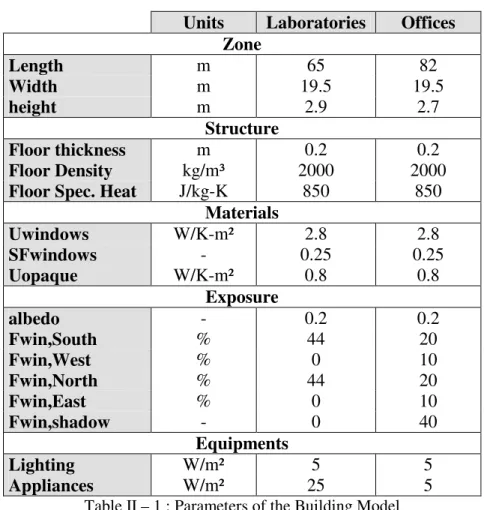
The simulation parameters for the both zones are presented in Table II-1.
Units Laboratories Offices Zone Length m 65 82 Width m 19.5 19.5 height m 2.9 2.7 Structure Floor thickness m 0.2 0.2 Floor Density kg/m³ 2000 2000
Floor Spec. Heat J/kg-K 850 850
Materials Uwindows W/K-m² 2.8 2.8 SFwindows - 0.25 0.25 Uopaque W/K-m² 0.8 0.8 Exposure albedo - 0.2 0.2 Fwin,South % 44 20 Fwin,West % 0 10 Fwin,North % 44 20 Fwin,East % 0 10 Fwin,shadow - 0 40 Equipments Lighting W/m² 5 5 Appliances W/m² 25 5 Table II – 1 : Parameters of the Building Model
U values correspond to the values used in the pre-audit. The thermal signature previously made has confirmed these hypotheses. Windows solar factor and albedo values are classical mean values (Lebrun, 2006b). Exposure factors and equipments loads have been estimated according to the actual geometry and installed appliances (As built File, 2003).
Once the studied zones are modelled, a simulation model must also be developed for the complete HVAC system.
II.3. HVAC System Model
As already said in the first part of this work, installed CAV (constant air volume) air handlers generally include air-to-air direct recovery loops, hot water heating coils, chilled water cooling coils, steam humidifiers and fans. In one zone (offices), classical heating & cooling terminal units are installed to ensure a permanent comfort temperature. All of these components will be now described and modelled.
Considering that the building model is a mono-zone model, all the models of the equipments of a given type (air handling units, terminal units…etc) can be gathered in a “global” model. Indeed, the different locations of the terminal units or of the air diffusers cannot be taken into account in a simplified mono-zone building model, it is so totally useless to differentiate the similar units. The global model is so composed of a mono-zone building model, a global air handling unit model (gathering the characteristics of the different AHU which are in charge of the zone) and a global terminal unit model (for the offices floor only). A last part of the model concerns the calculation of electrical and gas consumptions (using chiller and boiler models) and is only provided with cooling and heating demand previously calculated. These models will be presented below.
II.3.1. Air Handling Unit Model
The actual building is equipped with seven air handlers, installed in the Mechanical Equipment Room (MER). The equipments concerned by this work are referenced from GP/GE1 to GP5 and detailed in Table II-21.
AHU Mode Flow Rate
[m³/h] Zone GP/GE 1 100% fresh air 10000 Zone III (labs)
GP/GE 2 100% fresh air 11500 Zone III (labs)
GP/GE 3 100% fresh air 11500 Zone III (labs)
GP/GE 4 100% fresh air 5000 Zone I (offices)
GP 5 100% recirculated air 5000 Zone I (offices)
AHU Components
GP/GE 1 Filters – Recovery Loop– Cooling Coil – Heating Coil – Fan
GP/GE 2 Filters – Recovery Loop – Cooling Coil – Heating Coil – Steam Humidifier – Fan GP/GE 3 Filters – Recovery Loop – Cooling Coil – Heating Coil – Steam Humidifier – Fan GP/GE 4 Filters – Recovery Loop – Cooling Coil – Heating Coil – Fan
GP 5 Filters – Cooling Coil – Heating Coil – Steam Humidifier – Fan Table II – 2 : Components of the AHUs
characteristics. These characteristics will be used during simulations by a simplified (more robust) model. The other models are “orphan”, but simple models.
II.3.1.1. Heating Coil Model
In the considered installation, aluminium fin&tube coils, fed with hot water coming from the hot water network, are used to heat the air at the exhaust of the recovery coils. These devices are regulated thanks to the supply hot water temperature (controlled using a mixing three-way vane and a pump).
Complete “Mother” Model
Currently, (pre)heating coils are characterized by their heat transfer surface, composed of a primary (tubes external surface) and a secondary (fins external surface) heat transfer surface. The global heat transfer surface can be numerically represented by a global AU value of the coil. The aim of this first mother model is to determine the nominal AU value of the coil, corresponding to the nominal rating point, given by the manufacturer (Table II-3).
AHU GP/GE 1 GP/GE 2 GP/GE 3 GP/GE 4 GP 5 Heating Capacity [W] 85000 122000 122000 58000 15000
Air Flow Rate [m³/h] 10000 11500 11500 5050 5000
Entering Air Dry Temp. [°C] 3.6 2.3 2.3 -12 20
Entering Air Rel. Hum. [%] 25 27 27 90 50
Leaving Air Dry Temp. [°C] 28.9 33.9 33.9 22 28.9
Leaving Air Rel. Hum. [%] 5 4 4 7 29
Water Flow Rate [m³/h] 3.7 5.4 5.4 2.5 0.7
Entering Water Temp. [°C] 80 80 80 80 90
Leaving Water Temp. [°C] 60 60 60 60 70 Table II – 3 : Heating Coils Manufacturer Data
The main equations of the complete “mother” model are based on the classical ε-NTU method (Incropera & DeWitt, 1996; Ngendakumana, 2006)
First, the heat transfer must be expressed on both air (II.3.1) and water (II.3.2) sides.
The effectiveness of the heat transfer is expressed using the theoretical maximal heat transfer rate (II.3.3).
(II.3.1)
(II.3.2)
This effectiveness can be expressed as a function of the heat transfer coefficient AUheatingcoil, using the following formula (II.3.4).
The formula (II.3.4) corresponds to a counter-flow heat exchanger. In spite of the particular conception of heating coils, this approximation can be made for coils with more than 3 rows of tubes.
The obtained AU value also corresponds to the reverse of the total thermal resistance which exists between the air and the water flow rates. This total thermal resistance is also equivalent to three resistances disposed in series : the convective resistance on the airside, the conduction resistance of the metal and the convective resistance on the waterside.
The present model is implemented on “EES” and used for the five considered coils (Figure II-3). Specific heat and densities are computed using the property functions implemented in “EES” with air and water mean temperatures and at a standard atmospheric pressure of about
(II.3.4)
Figure II – 3 : Block Diagram Representation of the Heating Coil Model
AHU Coil AU value [W/K] Coil Effectiveness Heating Capacity [W] Leaving Air Temperature [°C] GP/GE 1 1557 0.3225 84149 28.24 GP/GE 2 2374 0.4054 122813 33.8 GP/GE 3 2374 0.4054 122813 33.8 GP/GE 4 861 0.3434 56858 19.59 GP/GE 5 287.9 0.2857 15851 29.55 Table II – 4 : Heating Coils Computed Characteristics
By comparing these results to the values given by the manufacturer (Table II-3), absolute and relative errors can be computed. Thus, leaving air temperature is calculated with an average absolute accuracy of about 0.7 °C. The heating capacity is computed with an average absolute accuracy of about 2%. Considering the simplicity and the fact that this model is currently used, no validation work will be realized for this model.
Simplified “Daughter” Model
To avoid difficult calculations and convergence problems, a simplified and robust model is extracted from the reference model. Two fair approximations are made in this secondary model :
1. the minimal capacity flow rate (eq. II.3.3) is supposed to be always the air capacity flow rate (which is currently the case),
2. the effectiveness of the heat exchanger is supposed to stay constant and equal to the previously computed value (Table II-4) during simulations.
The first approximation enables to avoid the use of the “min/max” functions and the calculation of the effectiveness using equation II.3.4, which could be problematic during simulations. Knowing that the air flow rate is maintained at constant level and that water flow rate stay equal to the nominal flow rate during functioning periods (CAV system with water temperature regulation), this hypothesis do not generate any errors. In the case of the air handler “GP 5”, the minimal capacity flow rate corresponds to the waterside and the approximation cannot be made. However, the functioning mode of this air handling unit (full recirculated air) allows us to consider it as a large terminal units. Its case will be treated in a following paragraph.
The second approximation does not induce any error if the both flow rates do not vary during simulation, what is the case in reality.
In this derived model, the heat transfer on waterside is not taken into account. Only two inputs are asked by the new model to calculate the exhaust air temperature (ta,ex,heatingcoil) : the supply hot water temperature (tw,su,heatingcoil, computed using regulation laws, allowing the follow-up of the set-point) and the supply air temperature.
Several pumps are used to control the heating load brought to the heating coils (Figure II-4). Table II-5 summaries the main characteristics of these pumps.
Pump AHU Number Flow Rate [m³/h] Manometric Height [m] Efficiency [%] Electrical Power [W] P4 GP1 1 3.7 2 21 100 P5 GP2 1 5.3 3 16 280 P6 GP3 1 5.3 3 16 280 P7 GP4 1 2.6 3 22 100 P8 GP5 1 0.7 3 8 70
Table II – 5 : Heating Coils Pumps Characteristics II.3.1.2. Cooling Coil Model
In the studied installation, several cooling coils are present in the different AHU. These cooling coils are typical aluminium fins&tubes cooling coils and are fed with chilled water coming from the chilled water network. Whereas no condensation risk has been taken into account in the case of heating coils, the appearance of condensate along the tubes and fins of cooling coils, in particular functioning conditions, must be modelled. Indeed, the cooling capacity is fully influenced by the (dry or wet) regime.
Manufacturer data for the installed cooling coils are presented in Table II-6.
AHU GP 1 GP 2 GP 3 GP 4 GP 5 Cooling Capacity [W] 61400 87400 87400 28200 16800
Sensible Power [W] 42000 57900 57900 20300 15000
Air Flow Rate [m³/h] 10000 11500 11500 5050 5000
Entering Air Dry Temp. [°C] 30 30 30 30 25
Entering Air Rel. Hum. [%] 50 50 50 50 50
Leaving Air Dry Temp. [°C] 17.5 15 15 18 16.1
Leaving Air Rel. Hum. [%] 89 98 98 90 84
Water Flow Rate [m³/h] 10.6 15 15 4.9 2.4
Entering Water Temp. [°C] 7 7 7 7 6 Figure II – 4 : Heating Coil Control System
Complete “Mother” Model
This reference (“mother”) model threats the cooling coil as a counterflow heat exchanger by using the model proposed by Lebrun & al. (1990), based on Merkel’s theory (F.Merkel, 1925). In this model, fully dry and fully wet regimes are described and computed simultaneously. According to Braun’s hypothesis (Braun, J.E., Klein, S.A., Mitchell, J.W., 1989), the regime to be considered is the one leading to the maximal cooling capacity.
According to this model, the cooling coil is finally characterized by three resistances disposed in series : the convective resistance on the airside, the conduction resistance of the metal and the convective resistance on the waterside.
In dry regime, the classical ε-NTU method is used to define the cooling capacity and the (dry) effectiveness. The overall heat transfer coefficient is calculated by considering the three thermal resistances previously quoted (equation II.3.5).
In wet regime, the air is replaced by a fictitious perfect gas, whose enthalpy is fully defined by the actual wet bulb temperature. The corresponding cooling power and (fictitious) thermal resistance are defined by equations (II.3.6) and (II.3.7).
(II.3.6)
(II.3.7) (II.3.5)
The air state at the cooling coil exhaust is computed by the means of a semi-isothermal heat exchanger, according to the ASHRAE classical procedure (ASHRAE, 2005). This fictitious heat exchanger is composed of the airflow on one side and of a fictitious fluid (of infinite capacity flow rate) on the other side. The supposed temperature of this fictitious fluid is called the “contact temperature” and corresponds to an “average” temperature of the external surface of the coil. The corresponding equations follow :
All the enthalpies, absolute humidity and wetbulb temperatures are defined using the very accurate functions already implemented and available in the solver library.
Using the data given in Table II-6, the model provides the following results (Table II-7). To identify the parameters of the model (thermal resistances), a guess must be made on the value of the metal thermal resistance. A fair approximation is to suppose the metal thermal resistance negligible opposite to the both convective thermal resistances.
AHU Air Thermal Resistance Water Thermal Resistance Cooling Capacity [W]
SHR
ε
dryε
wetε
contactGP 1 0.0001774 0.0001038 61487 0.68 0.6173 0.3499 0.8155
GP 2 0.00008542 0.00007419 87010 0.66 0.7661 0.4525 0.9522
GP 3 0.00008542 0.00007419 87010 0.66 0.7661 0.4525 0.9522
GP 4 0.0003418 0.000247 28423 0.71 0.5952 0.3479 0.8243
GP 5 0.0004285 0.0002833 16710 0.90 0.497 0.5044 0.7498 Table II – 7 : Cooling Coils Computed Characteristics
By comparing obtained cooling capacities and SHR values with the given nominal rating point data, relative errors can be computed. The cooling capacity and SHR are computed, respectively, with an accuracy of about 0.8% and 1.3%. These values are encouraging and have been confirmed by Lemort, Cuevas and Lebrun (2007) during a validation exercise realized with the concerned model.
The same authors also propose variations laws to compute the thermal resistances for variable air and water flow rates.
Simplified “Daughter” Model
Once more, a simplified model has been developed and extracted from the first model. The first simplification of the model consists in using simplified fluid properties in place of very accurate (but heavy) implemented functions available in the solver library. Simple (parabolic) correlations are identified for most of humid air state.
The second simplification is more specific and consists in not taking into account what happens on waterside. This is done by assuming the cooling coil exit air state is controlled by its contact temperature (in place of the chilled water flow rate). The minimal value of the contact temperature, corresponding to the full opening of the two-ways control valve, is determined as a function of water supply temperature and of dry or wet bulb air supply temperature (according to the dry or wet regime).
A third fair and convenient approximation is to “do as if” the transition between wet and dry regimes would occur exactly when the contact temperature is equal to the supply dew-point. These two last approximations can be justified by using simulation results obtained with the complete reference model (Lebrun, Lemort and Cuevas, 2007). In the considered example (Figure II-5), the transition is occurring for a water supply temperature of about 12.5°C, corresponding to as contact temperature of about 15.5°C. This last value is slightly below the supply dew point temperature (about 16.7°C).
In addition to these simplifications, the same suppositions as for the simplified heating coil model are made :
- the minimal capacity flow rate is supposed to correspond to the air side,
- the different efficiencies (dry, wet and contact) are supposed to stay constant and equal to the nominal efficiencies (calculated and given in Table II-7).
This model has already been validated and it appears that the loss of accuracy stay limited in the region corresponding to the transition between the two regimes (dry and wet). This lack of accuracy is probably not critical in a long-term simulation of a whole HVAC system.
Figure II – 5 : Evolution of the cooling coil power and contact temperature with the water supply temperature (Lemort et al., 2007)
The simplified model can be resumed in the following equations :
The regulation law is then used to compute the “used” contact temperature which is limited by the minimal contact temperature defined by equation (II.3.8). The exhaust air state is calculated using the following equations.