Science Arts & Métiers (SAM)
is an open access repository that collects the work of Arts et Métiers Institute of Technology researchers and makes it freely available over the web where possible.
This is an author-deposited version published in: https://sam.ensam.eu
Handle ID: .http://hdl.handle.net/10985/17515
To cite this version :
Fessal KPEKY, Komlan AKOUSSAN, Farid ABED-MERAIM, El Mostafa DAYA - Influence of geometric and material parameters on the damping properties of multilayer structures -Composite Structures - Vol. 183, n°1, p.611-619 - 2018
Influence of geometric and material parameters on the
damping properties of multilayer structures
Fessal Kpeky 2,3, Komlan Akoussan 4, Farid Abed-Meraim 2,3* and El-Mostafa Daya 1,3
1 LEM3, UMR CNRS 7239, Université de Lorraine, Ile du Saulcy Metz Cedex 01, France 2 LEM3, UMR CNRS 7239, Arts et Métiers ParisTech, 4 rue A. Fresnel, 57078 Metz Cedex 03, France
3
Laboratory of Excellence on Design of Alloy Metals for low-mAss Structures (DAMAS), France
4 LEMTA, UMR CNRS 7563, Université de Lorraine, Mines Nancy, GIP-InSIC, 27 rue d’Hellieule, 88100
Saint-Dié-des-Vosges, France
Abstract. In this paper, we investigate the influence of deviations in the design and
implementation parameters on the damping properties of multilayer viscoelastic structures. This work is based on a numerical approach, which uses recently developed solid–shell elements that have been specifically designed for the modeling of multilayer structures. The originality in the current study lies in the analysis of variation in the design parameters, which could be of geometric or material type. Indeed, although several models have been proposed to study variability, they remain mostly complex to implement. Our approach is rather simple, and is based on the uncertainty on the actual values of several parameters in some well-defined intervals. The developed method is applied to the vibration modeling of multilayer structures, with elastic faces and viscoelastic core material. The resulting problem is discretized by using quadratic solid–shell finite elements. To solve the associated nonlinear equations, we adopt the method that couples the homotopy technique to the Asymptotic Numerical Method (ANM) as well as the Automatic Differentiation (AD) and path continuation. The obtained results provide useful information on the error tolerance margin that could be allowed without compromising structural integrity.
Keywords: Multilayer structures, Sensitivity analysis, Solid–shell finite elements, Vibrations,
Viscoelasticity, Asymptotic numerical method.
1. Introduction
Vibration and noise control is of crucial importance in a number of engineering domains. Indeed, vibration issues may be encountered in automotive industry, aeronautics, navy, civil infrastructures, etc. and, in many situations, they cause discomfort or system dysfunction and may even lead to failure of structures. To reduce vibrations, thus avoiding their detrimental
more complex composite structures (honeycombs [3, 4], viscoelastic inclusions embedded in an elastic matrix [5, 6], etc.). Moreover, viscoelastic materials are lightweight and, as such, they contribute to weight reduction for the structures in which they are used. It is therefore important to precisely identify the characteristics of viscoelastic materials as well as their damping properties for their proper implementation. The key damping features of viscoelastic structures are closely related to the mechanical characteristics (Young’s modulus, Poisson’s ratio) of the constituent materials, as well as to the geometric dimensions (layer thicknesses, structure length and width, aspect ratios, etc.) [7, 8]. Also, when the viscoelastic faces of sandwich structures are made of laminates, the resulting damping properties are linked to the fiber orientation angles [7, 9]. In the related literature, there have been several studies dedicated to the calculation of the damping properties of viscoelastic sandwich structures. Earlier contributions to the field were restricted to viscoelastic sandwich structures with isotropic layers [10-13]. Subsequent works focused on the modeling of viscoelastic sandwich structures with laminated faces, since laminates can be manufactured for a specific need [ 14-16]. The numerical tools developed in these various works are aimed at predicting the main characteristics of viscoelastic structures, in order to assist engineers in the design process. However, in the manufacture stage of viscoelastic structures, it is quite common that designers face issues related to uncertainty in the mechanical characteristics and geometric dimensions of the structure under design. In general, two types of uncertainties are usually known to affect the manufacture of viscoelastic sandwich structures, which are sometimes designated as imperfections. The first type of these imperfections generally results from the manufacturing process of these structures [17], meaning potential errors made on their geometric dimensions (e.g., thickness of layers, length, width, aspect ratios …). The second source of variation arises from the mechanical parameters of the constituent materials, as identified in the literature (e.g., aluminum Young modulus taken equal to 70.3 GPa in [18], while identified to 69 GPa in [19]). Because such imperfections directly affect the damping properties of structures, it is therefore of major importance to quantify the impact of these uncertainties, in order to guaranty optimal damping characteristics and proper final in-use properties. To this end, several studies have been proposed in the literature, among which the contribution of Hu et al. [20], who proposed a comprehensive review on sandwich structure modeling theories. More specifically, in Hu et al. [20], relevant comparisons have been made, which involve various kinematic approaches for sandwich structures, through a study of the influence of different parameters, including the ratios of core to face thickness (hc/hf ), slenderness (L h/ ), and Young’s modulus (Ec/Ef ). More recently, Hamdaoui et al. [21] proposed a study where the Modal Stability Procedure (MSP) has been combined with the Monte Carlo Simulation (MCS). Although a number of existing methods are effective for variability analysis, they are essentially based on a discrete calculation and, hence, are time consuming. The complexity of the strongly nonlinear eigenvalue problems, which result from the modeling of viscoelastic sandwich structures, requires the development of new numerical methods that are both capable of continuously solving the resulting nonlinear problem and computationally efficient. In this context, worth mentioning is the work of Duigou et al. [22], who proposed two iterative algorithms to solve nonlinear eigenvalue problems. Their method has been made more robust and generic by the introduction of Automatic Differentiation (AD)
[23-25]. Despite its robustness, this method remains limited since it allows computing only one pair of solutions at a time, namely the natural frequency and the loss factor. The use of such an approach to solve our problem would require considerable CPU times, as the associated numerical technique would have to be applied incrementally over the whole range investigated.
In the current work, we present finite element models based on the solid–shell approach, which have been specifically designed for the modeling of multilayer structures. The originality in the current study lies in the analysis of variation in the design parameters, which could be of geometric or material type. This approach is rather simple, and is based on the uncertainty on the actual values of several parameters in some well-defined intervals. The developed method is applied to the vibration modeling of multilayer structures, which consist of elastic faces and viscoelastic core material. The resulting problem is discretized by using solid–shell finite elements, which have been developed in [26, 27] and recently extended to viscoelastic sandwich structures in [13]. For the analysis of variability with regard to a given parameter, the associated nonlinear eigenvalue problem depends both on the frequency and on the selected parameter. Also, the range of variation of each selected parameter is restricted to an interval, which will be referred to as the study interval. In order to continuously solve the corresponding nonlinear equations, we adopt the method that couples the homotopy technique to the Asymptotic Numerical Method (ANM) as well as the Automatic Differentiation (AD) and path continuation procedure (see, e.g., [7, 28]). The obtained results provide useful information on the error tolerance margin that could be allowed without compromising structural integrity.
2. Formulation and discretization of the problem
2.1. Governing equations and their discretization
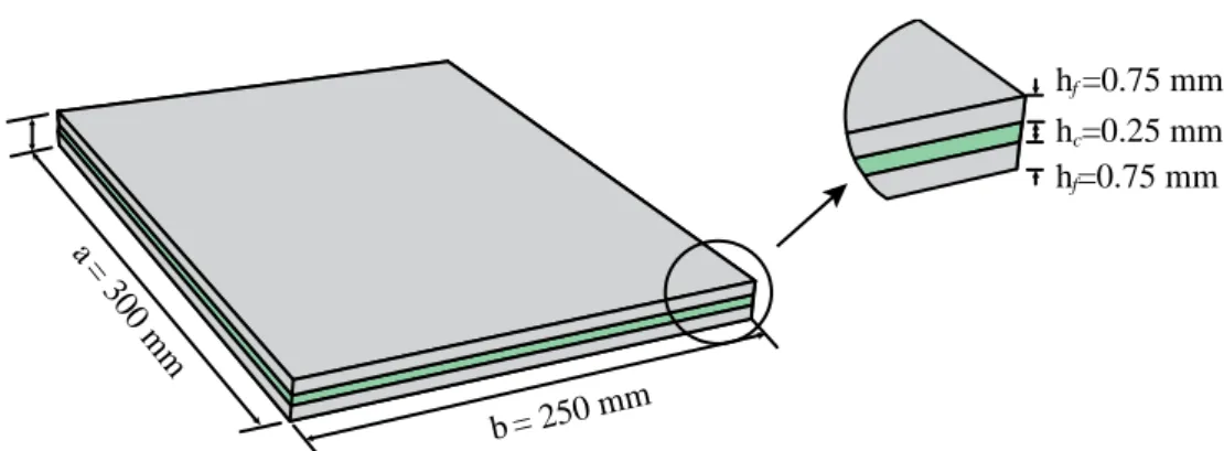
In this work, we consider the free vibration problem of a multilayer structure, as illustrated in Fig. 1. The virtual work principle governing the equilibrium of such a structure is given as follows:
(
:)
d 0V
δ
+ρ δ
⋅ v=∫
σ ε
uɺɺ u , (1)where
σ
,ε
and u are, respectively, the stress and strain tensors, and the generalized displacement at a point within the body V of the viscoelastic structure, while the density of the material is denoted byρ
. The stress and strain tensorsσ
andε
as well as the displacement u can be expressed as harmonic time functions.Fig. 1. Sandwich plate with elastic faces and viscoelastic core material.
The viscoelastic damping behavior is accounted for through the stress–strain constitutive law, which can be written in the form:
( ) : with ( )
ω
ω
R( )ω
i I( )ω
=C C =C + C
σ
ε
, (2)where CR( )
ω
and CI( )ω
are, respectively, the tensors characterizing the energy storage and dissipative behavior of the viscoelastic material.Combining Eqs. (1) and (2), and using a finite element discretization, the natural vibration problem of viscoelastic structures can be written in the following form:
{ }
2 ( )
ω ω
=
K − M U 0, (3)
where K and M denote, respectively, the stiffness and mass matrix of the structure, and the complex nodal vibration eigenmode is denoted by U. The above matrices are obtained by finite element discretization using the solid–shell elements SHB20 and SHB15. The formulation of these two solid–shell elements is briefly outlined hereafter, the interested reader may refer to [27, 13] for the complete details.
2.2. Solid–shell finite element formulation 2.2.1. Kinematics and interpolation
The above-described vibration problem is discretized using the solid–shell finite elements SHB20 and SHB15, originally proposed by Abed-Meraim et al. [27]. These SHB20 and SHB15 elements denote a twenty-node hexahedral element and a fifteen-node prismatic element, respectively. Based on a fully three-dimensional approach, these elements have only three displacement degrees of freedom per node. Nevertheless, to improve the performance of
Elastic layers Viscoelastic layer
these solid–shell elements, and to provide them with some desirable shell features, a number of enhancements are introduced within their formulations based on the assumed-strain method (ASM). In particular, a special direction is chosen, designated as the “thickness”, normal to the mean plane of these elements, along which a user-defined number of integration points are arranged. Also, an in-plane reduced-integration rule is used, with 4 n× int integration points for the SHB20 element and 3 n× int for the SHB15 (see, e.g., Fig. 2, in the particular case when the number of through-thickness integration points is nint =5).
Fig. 2. Schematic representation for the reference geometry of the SHB20 and SHB15
elements as well as for the location of their integration points in the case when the number of through-thickness integration points is nint=5.
For the SHB20 and SHB15 elements, the spatial coordinates xi are related to the nodal coordinates xiJ using the conventional quadratic shape functions, as follows:
(
, ,)
i iJ J
x =x N ξ η ζ , (4)
where i represents the spatial directions and ranges from 1 to 3; while J stands for the node number, which ranges from 1 to 20, for the SHB20 element, and from 1 to 15 for the SHB15. Likewise, the displacement field ui is related to the nodal displacements uiJ using the same quadratic shape functions:
(
, ,)
i iJ J
u =u N ξ η ζ . (5)
Note that in Eqs. (4) and (5) above, the convention of implied summation over the repeated index J has been adopted.
ξ ζ 5 1 2 3 4 1 2 3 4 5 6 7 8 10 9 11 14 15 16 20 19 18 17 13 12 6 7 8 9 10 11 12 13 14 15 16 17 18 19 20 η 2 1 3 5 4 6 ξ η ζ 1 2 3 4 5 15 7 9 13 8 11 10 12 14 6 7 8 9 10 11 12 13 14 15
2.2.2. Discrete gradient operators
For both elements SHB20 and SHB15, the corresponding discrete gradient operator
[ ]
B
can be derived in the following compact form:
1 ,1 2 ,2 3 ,3 2 ,2 1 ,1 1 ,1 3 ,3 3 ,3 2 ,2 T T T T T T T T T T T T T T T T T T h h h h h h h h h α α α α α α α α α α α α α α α α α α + + + = + + + + + + 0 0 0 0 0 0 B 0 0 0 b γ b γ b γ b γ b γ b γ b γ b γ b γ , (6)
where biT , hα,i and γαT have been fully detailed in [27]. Note again that, in Eq. (6) and in what follows, the convention of implied summation over the repeated index
α
is adopted, withα
ranging from 1 to 16, for the SHB20 element, and from 1 to 11 for the SHB15.The discrete gradient operator given by Eq. (6) allows us to compute the stiffness matrix for each of the SHB20 and SHB15 solid–shell elements. In the same way, the corresponding mass matrices, involved in the vibration problem governed by Eq. (3), are easily computed using the classical shape functions associated with these quadratic elements. Once the governing equations have been discretized in the form of Eq. (3), it is relevant to develop an effective method for solving the associated nonlinear problem, which will be the object of the next section.
3. Numerical resolution method
The simplest approach to solve the above-described nonlinear governing equations is to use the incremental method, which consists in performing computation for each value of the design parameter in its predefined range of variation. However, such an approach has two main drawbacks. On the one hand, it requires a huge amount of CPU time, due to the number of points to be chosen in the analysis range for a more efficient result. On the other hand, this method may not distinguish singular points that would represent optimums. To overcome these limitations, the generic numerical resolution method, which has been proposed by Akoussan et al. [7] and applied to thickness sensitivity analysis, is adopted here. This method consists in recasting the frequency-dependent nonlinear eigenvalue problem, as defined by Eq. (3), into a nonlinear eigenvalue problem depending both on the frequency and on the modeling parameter (see Eq. (7) below). The new resulting problem is then continuously solved using a method that couples the homotopy technique to the ANM as well as the AD and path continuation procedure [23-25].
{ }
2
(
ω
,p)ω
( )p , p I = ∈
In this Eq. (7), p represents the selected modeling parameter, whose variation will be analyzed, and I is the interval in which this parameter will vary (denoted hereafter as the study interval). Generally, the stiffness and mass matrices involved in Eq. (7) are expanded in the form of Eq. (8) below, in order to avoid differentiation of large size matrices, which would give rise to computational memory issues and substantial computation times during the calculations.
[
]
[
]
[ ]
* * 1 1 ( , ) ( , ) ( ) ( ) ( ) ( , , ) Q gq q g g q L ml l m g l p E p E p p E p E pλ
λ
λ
= = = = = = ∑
∑
K K K M M M (8)where Egq* (
λ
,p) and Eml( )p are analytical functions of the modeling parameter p, and the associated constant matrices are denoted Kq and Mj, respectively. Adopting such a transformation, the differentiation of the stiffness and mass matrices simply reduces to the differentiation of the analytical functions Egq* (λ
,p) and Emj( )p .In what follows, the main lines of this solution procedure will be described.
3.1. Residual problem
To solve the nonlinear eigenvalue problem given by Eq. (7), using the generic method developed in [7], the problem is first transformed into a residual eigenvalue problem by setting λ ω= 2 and applying the decomposition depicted above for the stiffness and mass matrices, which gives:
{ }
*
( ,
λ
,p)=Eg(λ
,p) g −λ
Em(p) g = , p∈IR U K M U 0 . (9)
A perturbation technique δp is then applied to the modeling parameter p. The eigenpair is additionally developed as Taylor’s expansions of δp, truncated at a user-defined order N:
(
)
(
)
0 ( ) ( ) ( , )( ) ( ) ( , , ( ) , ( ) )( ) 1 1 ( , )( ) ! ! , n n n n n N n n n n n p p p p p p n n p pλ
λ
λ
δ
δ
λ
λ
= ∂ + = = = ∂∑
U U U U U (10)The residual problem is similarly expanded into a Taylor series form, by introducing the Taylor expansion of the eigenpair ( , )U λ as follows:
(
)
(
)
(
)
(
)
0 ( ), ( ), ( ( ), ( ), 1 ( ), ( ), ( ( . ) ), ), ! n N n n n n n p p p p p p p p p p p p p p n pδ
δ
λ
λ
λ
λ
= = ∂ ∂ + = =∑
R R 0 R R U U U U (11)By identifying the terms of same power in δp, the residual problem is sent into a recurrence form, which needs to be solved for each value of n (0≤ ≤n N )
{
}
{
10 1} {
1 1}
{
}
0 0| 0 1| , 0 1| , 1 | n , n 0 , 1. Id n dλ n λλ
n n λ n = = = = = = = = = = = + 0 + 0 ≥ R R 0 R R R R 0 U U I U U U U (12)3.2. Resolution of the residual problem at order 0
The residual problem at order n =0 is written explicitly as:
(
)
0{ }
(
)
( )
{ }
*
0 0,
λ
0,p = 0| =d 0 =Egλ
0,p g −λ
0Em p g 0 =R U R U I U K M U 0, (13)
which is a nonlinear frequency-dependent eigenvalue problem, since the analytical function to be differentiated depends on the unknown
λ
0. Another difficulty in this Eq. (13) is the choice of the departure value for the modeling parameter, which varies within the study interval I . This departure value can be chosen as being the upper bound or the lower bound of the study interval. This choice should however be motivated by a preliminary study, since in some cases, choosing the upper bound as departure value for the modeling parameter allows reducing the computation times as compared to the case when the lower bound is chosen. In practice, the Young modulus of the viscoelastic layer of the sandwich structure is decomposed into two parts:(
)
( )
(
)
* * , 0, ,λ
= +λ
g g g E p E p E p , (14)where E*g(0, )p represents the delayed elasticity of the core.
Let us take as appropriate departure value for the modeling parameter p= p0. The residual problem given by Eq. (13) becomes:
(
)
(
)
(
*)
( )
{ }
0( 0,
λ
0, 0)= 0, 0 +λ
0, 0 K −λ
0 0 M 0 =0R U p Eg p Eg p g Em p g U . (15)
This residual problem can be solved by any numerical method dedicated to solving nonlinear frequency-dependent eigenvalue problems. A representative selection of these methods has been presented and compared in [29]. In the current work, the above nonlinear eigenvalue problem, which allows computing the first eigenpair (U0,
λ
0), is solved by using the method that couples the homotopy technique to the Asymptotic Numerical Method as well as the Automatic Differentiation and path continuation procedure. This method consists intransforming the residual problem at order 0 into a new problem, which is split in turn into two sub-residues:
(
)
(
)
(
) (
)
(
)
[ ]
(
)
(
)
( )
(
)
(
)
0 0 0 0 0 0 * 0 0 0 , , , , , 1 , , , , , , 0,1 , 0, , , , h h g g m g g g p p a p a a a E p E p E pλ
γ
γ
γ
γ
γ
γ
γ
γ
= = = = + = ∈ = − = 0 0 K R R R S T S M K T U V V V V V V V V (16)where a is the homotopy parameter. The new functions and unknowns are then expanded in Taylor’s series of the homotopy parameter a , which are truncated at the order N. Inserting their expressions into the new residual problem Rh allows deriving a generic linear system to be implemented into the DIAMANT Toolbox. This generic form is obtained using the derivative chain rule with suitable initialization, in order to first compute the unknown
γ
i by the following expression:{
} {
}
{
1 1} {
1 1}
0 | , 0 | , 0 1 0 1| , 1 1| , 1 , 1, 2,..., i i i i t i i i i t a N a i γ γ γ γγ
= = = = − = = = = + + = − = + 0 0 0 0 V V V V V S T T V S T , (17)and to use the obtained value for this unknown in the following system to get the second unknown Vi:
{ } { }
{ }
0 i| i| 1 0 , 1, 2,..., 0 0 i i i i t a N iχ
= = − − − − = = 0 0 A V V SV TV T V , (18)where A=E*g(0,p0)Kg −
γ
Em(p0)Mg+aEg( ,γ
p0)Kg is the linear tangent matrix andχ
is the Lagrange multiplier. The iterative solution(
V,γ
)
is then determined using the continuation procedure until a ≥1. Finally, the eigenpair solution of the residual problem at order 0 is computed by:(
0 0)
(
) (
)
0 , 1 , N i i i i aλ
γ
= =∑
− U V . (19)More details about this resolution procedure can be found in [24, 30].
3.3. Resolution of the residual problem at order n
Once the first eigenpair
(
U0,λ
0)
has been obtained by solving the residual problem at order 0, the residual problem R is solved at each order n to determine the other eigenpairsince it represents one equation with two unknowns Un and
λ
n. To solve this equation, the mode orthogonality condition (see Eq. (20) below) is added:(
)
0 0 0
t − =
U U U . (20)
From the two Eqs. (12) and (20), a generic system is built at each iteration n:
{
1 1}
{
}
0 1| , 1 | , 0 0 0 0 n n n n t t n λλ
λχ
= = = = − − = 0 0 K U U RU R U U . (21)Before solving this system, the value of
λ
n is first calculated by using the following generic Eq. (22): 1 1 0 | , 0 0 1| , 1 n n n t t n λ λλ
= = = = = − 0 0 U U R U R U . (22)In the generic system given by Eq. (21), Kt =
(
Eg*(0,p0)+Eg(λ
0,p0))
Kg −λ
0Em(p0)Mgrepresents the linear tangent matrix of the series. At the end of each series, the convergence radius is evaluated using a precision parameter
ε
, provided by the user (see Eq. (23) below), which will allow the modeling parameter p to be updated:1 1 1 N N p
δ
=ε
− U U . (23)This update is achieved in two different ways, according to the choice of the departure value for the modeling parameter p. Hence, when the departure value is taken to be the upper bound of the study interval, the modeling parameter is updated as follows:
0 0 = −
δ
p p p, (24)
otherwise, when the departure value is taken to be the lower bound, the update of the modeling parameter is achieved as follows:
0 = 0+
δ
p p p. (25)
In case the update Eq. (24) is used, if the convergence radius computed by Eq. (23) does not allow covering the study interval, a new branch of series is built, and its starting values are obtained from the former series as follows:
(
0 0)
(
) (
)
0 , , N n n n n pλ
δ
λ
= =∑
− U U , (26)otherwise, when the update Eq. (25) applies, the new series, when required, is built using the following stating values:
(
0 0)
( ) (
)
0 , , N n n n n pλ
δ
λ
= =∑
U U . (27)Finally, the damping properties, namely the damped frequency Ω and the loss factor η, are obtained from the eigensolution λ as follows:
(
)
2 2 1 ,ω
η
λ
λ
λ
λ
λ
η
λ
= Ω + = + = Ω = = R I I R R i i . (28)4. Results and discussions
The interest and the effectiveness of the proposed numerical tool are shown in this section through a set of representative benchmark tests. For all subsequent analyses, we consider as a reference problem a sandwich plate with elastic faces and viscoelastic core material. This sandwich plate is clamped at all of its four edges, as illustrated in Fig. 3. The viscoelastic core is made of ISD112-27°C. The properties of the adopted materials, both in the elastic layers and in the viscoelastic core, are reported in Table 1. The viscoelastic behavior of the core material is described, based on generalized Maxwell’s model, by:
( )
0 3 1 1 j j j G G iω
ω
ω
= ∆ = + − Ω ∑
, (29)where G0 is the shear modulus of the delayed elasticity, while the remaining parameters (∆ Ωj, j) are reported in Table 2.
Fig. 3. Sandwich plate with the initial geometric properties.
hf=0.75 mm hf=0.75 mm hc=0.25 mm b = 250 mm a = 3 00 m m
Table 1. Material properties of the constituent materials. Elastic layers 3 ρ =2766 Kg m E =69.0 GPa = 0.3 f f f ν − ⋅ Viscoelastic layer 0 0 0 -3 c c c ρ =1600 Kg m E =1.49 MPa = 0.49 ν ⋅
Table 2. Viscoelastic parameters of the ISD112-27°C material.
j ∆j -1 (rad.s ) j Ω 1 0.746 468.7 2 3.265 4742.4 3 43.284 71532.5
The aim of this study is to assess the influence of variation in a number of parameters on the damping properties of the above-described sandwich structure. In this analysis, we will limit ourselves to five main distinct parameters associated with the viscoelastic core layer:
- the thickness variation, - the Young modulus variation, - the Poisson ratio variation, - the density variation, - the temperature variation.
For the sake of comparison, all of the subsequent simulations are performed using three different finite element discretizations. The latter consist of the proposed quadratic solid–shell elements SHB15 and SHB20, with 15 and 20 nodes, respectively, as well as the standard quadratic 20-node solid element HEX20. For all of the simulations, the mesh nomenclature adopted for the hexahedral elements is as follows: N
(
1×N2×N3)
elements, whereN
1denotes the number of elements in the length direction,
N
2 is the number of elements in the width direction, andN
3 is the number of elements in the thickness direction. For the prismatic element, however, the adopted mesh nomenclature is(
N1×N2×N3)
×2, where the multiplication by 2 is due to the subdivision of each original hexahedron into two prisms. Note also that, for the proposed solid–shell elements SHB15 and SHB20, two integration points along the thickness direction are sufficient for the following computations, as the corresponding benchmark tests do not involve material nonlinearities. However, it must benoted that, when nonlinear material behavior models enter into play, more through-thickness integration points are required (for instance, five through-thickness integration points are recommended when elasto-plastic constitutive models are used, see, e.g., reference [26]).
4.1. Variation of core thickness
For this first analysis, the incremental method is exceptionally used, due to the mesh dependence of the problem. Indeed, the fully 3D finite element modeling adopted here does not allow for an analytical expression for the thickness dependence of the problem, as can be done in some particular situations (e.g., an example of such an analytical expression has been achieved within a 2D finite element modeling framework [7]). This first test will also enable us, among other things, to bring out some limitations of this finite element method, which have been already mentioned before.
We investigate the influence of the core thickness
0 50%
c c
h =h ± on the damping properties of the sandwich structure. Thirty points have been taken to cover the interval of study. The results are presented in Fig 4 for the three different finite element discretizations discussed above. In terms of finite element performance, it can be observed that the proposed solid–shell elements are generally more efficient, as compared to the standard solid element HEX20, especially the hexahedral SHB20 element, which requires coarser meshes (i.e., four times less elements) for comparable accuracy. The analysis of the curves reported in Fig. 4 also shows that the frequencies decrease slightly with the increase in the core thickness. Indeed, this frequency reduction is of 14% for the first mode, and of 13% for the third one. There is also a decrease in the loss factors as the core thickness increases. For the first mode, the loss factor increases very slightly to a core thickness of bout hc =0.14, before decreasing almost linearly. The loss factors for the second and third modes decrease more noticeably (a decrease ranging from about 14% to 17%). From this analysis, it can be concluded that a larger thickness for the viscoelastic core layer does not necessarily enhance the damping properties as one might think.
Moreover, it comes from this first analysis that the incremental method, although simple to implement, does not make it possible to identify singular points.
Fig. 4. Sensitivity of the damping properties to the core thickness.
In all of the following analyses, it is the resolution method presented in section 3 that will be used.
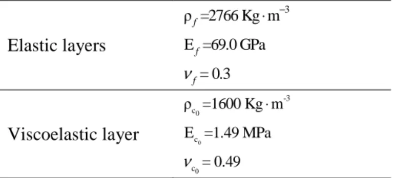
4.2. Variation of the Young modulus of the core material
In this subsection, we analyze the influence of a 50% variation on the Young modulus of the viscoelastic core material on the damping properties of the sandwich structure. For this purpose, Eq. 7 can be rewritten in the following form:
(
)
{ }
1 2 1 0 2 0 2 , , , where 0.5 and 1.5 , R C C C C C C C C C E E I E E E E E Eω
ω
+ − = ∈ = = × = × K K M U 0 (30)One of the main benefits brought by the new numerical method is that the user only needs to define the matrices KR, KC, M, the bounds
1 C E and
2 C
E of the investigated modeling variable, as well as the desired precision δ . As outputs from the analysis, the user obtains in a straightforward way the damping parameter curves f E( C) and
η
(EC).The results plotted in Fig. 5 show a more or less significant increase in the damping parameters. Indeed, this increase is quasi-linear for the first three frequencies (21% for the first frequency, and 16% for the third frequency). On the other hand, there is a very marked increase in the loss factors of the three modes investigated. This increase ranges from 72% for the first mode to 105% for the third mode. Overall, this analysis reveals that the damping parameters increase with the Young modulus of the viscoelastic core material.
0.1 0.15 0.2 0.25 0.3 0.35 0.4 100 150 200 250 300
Thickness of the core (mm)
F re q u e n c y ( H z ) 0.1 0.15 0.2 0.25 0.3 0.35 0.4 0.26 0.28 0.3 0.32 0.34 0.36
Thickness of the core (mm)
L o ss f a c to r HEX20 − 24×20×3 SHB15 − (12×10×3)×2 SHB20 − 12×10×3 Mode 1 Mode 2 Mode 3 HEX20 − 24×20×3 SHB15 − (12×10×3)×2 SHB20 − 12×10×3 Mode 1 Mode 2 Mode 3
Fig. 5. Sensitivity of the damping properties to the Young modulus of the core material.
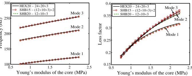
4.3. Variation of the Poisson ratio of the core material
Here, the effect of the Poisson ratio of the viscoelastic core material on the damping properties of the sandwich structure is investigated. The interval of study is set as follows:
[
0.1, 0.5
]
CI
ν
∈ =
. For this analysis, Eq. (7) can be rewritten as:(
)
2{ }
[
]
, , 0.1, 0.5
R C
ω ν
Cω
ν
C I + − = ∈ =
K K M U 0 . (31)
The analysis of the curves plotted in Fig. 6 reveals a relatively small decrease in the damping parameters. Indeed, this reduction is quasi-linear, and quite weak for the first three frequencies (around 5%). With regard to the loss factors, we observe a monotonous decrease until
ν
C =0.48, followed by a slight increase. Overall, within the interval of analysis ranging between the above-defined two bounds, the loss factor is reduced by 9% for the first frequency, and 13% for the third one.From this analysis, one can conclude that the more incompressible the core material, the less effective the corresponding damping.
0.5 1 1.5 2 2.5 100 150 200 250 300
Young’s modulus of the core (MPa)
F re q u e n c y ( H z ) 0.5 1 1.5 2 2.5 0.2 0.25 0.3 0.35 0.4
Young’s modulus of the core (MPa)
L o ss f a c to r HEX20 − 24×20×3 SHB15 − (12×10×3)×2 SHB20 − 12×10×3 Mode 1 Mode 2 Mode 3 HEX20 − 24×20×3 SHB15 − (12×10×3)×2 SHB20 − 12×10×3 Mode 1 Mode 2 Mode 3 0.15
Fig. 6. Sensitivity of the damping properties to the Poisson ratio of the core material.
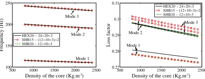
4.4. Variation of the density of the core material
This fourth type of analysis is concerned with the investigation of the impact of density variation, within the interval
0 50%
C
ρ
± , on the damping properties of the sandwich structure. For this analysis, Eq. (7) is rewritten in the form:( )
(
) { }
1 2 1 0 2 0 2 , , where 0.5 and 1.5 , R C C C C C C C C F C C Iω
ρ
ρ
ρ
ρ
ω
ρ ρ
ρ
ρ
+ − + = ∈ = = × = × K K M M U 0 (32)The results of this study, which are depicted in Fig. 7, reveal a slight variation of the damping parameters. Indeed, the curves plotted in Fig. 7 show a very small linear decrease in both the frequencies and the loss factors for the first three modes investigated. This reduction is of about 4% for the first three frequencies, and of about 2% for the corresponding loss factors. It can be concluded that the reduction in the mass density of the viscoelastic core material has a very small impact on the damping capabilities of the host structure. This result may reveal useful for the design of lightweight structures, while maintaining effective damping properties. 0.1 0.2 0.3 0.4 0.5 100 150 200 250 300
Poisson’s ratio of the core
F re q u e n c y ( H z ) 0.1 0.2 0.3 0.4 0.5 0.26 0.28 0.3 0.32 0.34 0.36
Poisson’s ratio of the core
L o ss f a c to r HEX20 − 24×20×3 SHB15 − (12×10×3)×2 SHB20 − 12×10×3 Mode 1 Mode 2 Mode 3 HEX20 − 24×20×3 SHB15 − (12×10×3)×2 SHB20 − 12×10×3 Mode 1 Mode 2 Mode 3
Fig. 7. Sensitivity of the damping properties to the density of the core material.
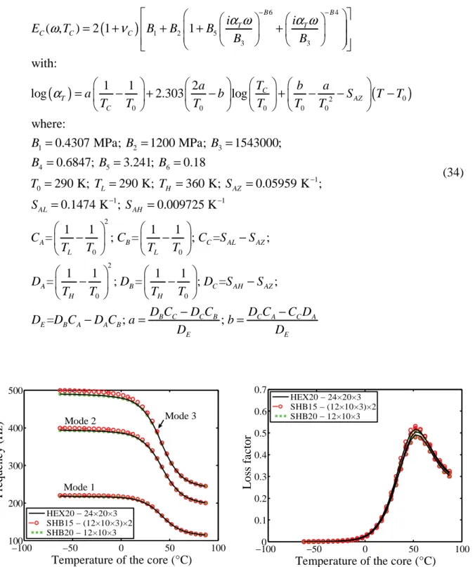
4.5. Influence of temperature variation
This last test is devoted to the analysis of the influence of the variation of the temperature of the viscoelastic core material on the damping properties of the sandwich structure. For the sake of simplicity, it will be assumed that the variation of temperature only affects the viscoelastic layer. The analysis is carried out for a modeling parameter (here the temperature) ranging in the interval I = − ° °
[
63 ;87]
. In this special case, Eq. (7) can be rearranged in the following form:(
)
2{ }
[
]
63 , 8 , , 7 R Cω
TCω
TC I + − = ∈ = − ° K K M U 0 ° . (33)The viscoelastic modulus of the ISD112 material, which takes into account the double frequency-temperature dependence, is given by the following relations (see [31]):
500 1000 1500 2000 2500
100 150 200 250
Density of the core (Kg.m-3)
F re q u e n c y ( H z ) 500 1000 1500 2000 2500 0.27 0.28 0.29 0.3 0.31
Density of the core (Kg.m-3)
L o ss f a c to r HEX20 − 24×20×3 SHB15 − (12×10×3)×2 SHB20 − 12×10×3 Mode 1 Mode 2 Mode 3 HEX20 − 24×20×3 SHB15 − (12×10×3)×2 SHB20 − 12×10×3 Mode 1 Mode 2 Mode 3
(
)
( )
(
)
6 4 1 2 5 3 3 0 2 0 0 0 0 0 1 2 3 4 ( , ) 2 1 1 with: 1 1 2 log 2.303 log where: 0.4307 MPa; 1200 MPa; 1543000; 0.6 C B B T T C C T A C Z C i i E T B B B B B a T b a a b S T T T T T T T T B B B Bα ω
α ω
ω
ν
α
− − = + + + + = − + − + − − − = = = = 5 6 1 0 1 1 2 0 0 2 0 0 847; 3.241; 0.18 290 K; 290 K; 360 K; 0.05959 K ; 0.1474 K ; 0.009725 K 1 1 1 1 = ; = ; = ; 1 1 1 1 = ; = ; = ; L H AZ AL AH A B C AL AZ L L A B C AH AZ H H B B T T T S S S C C C S S T T T T D D D S S T T T T D − − − = = = = = = = = − − − − − − = ; B C C B; C A C A E B A A B E E D C D C D C C D D C D C a b D D − − − = = (34)Fig. 8. Sensitivity of the damping properties to the temperature of the core material.
The simulation results relating to the influence of temperature are reported in Fig. 8. A decrease in frequencies over the entire interval is observed, whereas the loss factors increase to a peak value, before decreasing beyond this limit. Indeed, the damping parameters remain almost unchanged for temperature values lower than 0°C, which corresponds to the temperature range where the viscoelastic core is frozen and rigid. This also explains the high values for the frequencies and quasi-zero value for the loss factors, which describe the
−100 −50 0 50 100 100 200 300 400 500
Temperature of the core (°C)
F re q u e n c y ( H z ) −1000 −50 0 50 100 0.1 0.2 0.3 0.4 0.5 0.6 0.7
Temperature of the core (°C)
L o ss f a c to r HEX20 − 24×20×3 SHB15 − (12×10×3)×2 SHB20 − 12×10×3 HEX20 − 24×20×3 SHB15 − (12×10×3)×2 SHB20 − 12×10×3 Mode 1 Mode 2 Mode 3
damping properties. From 0°C, the core in ISD112 material becomes more viscous, which very rapidly leads to an increase in the loss factors and a decrease in the frequencies, since the rigidity of the structure drops. Beyond 53.4°C, the viscoelastic core material becomes less and less viscous and the damping capability begins to fall. This phenomenon explains the decrease in the loss factors (see Fig. 8). As to the frequencies, the latter stabilize towards their lowest values, as the contribution of the viscoelastic core to the rigidity of the structure becomes quasi constant.
The results of this analysis of temperature effect are particularly interesting in the search for optimal damping, which is identified here at a temperature of 53.4°C for this specific configuration of sandwich structure.
5. Conclusions
In the current contribution, the sensitivity analysis of the damping properties of a sandwich plate with viscoelastic core has been carried out for a selected set of representative modeling parameters. The sandwich structure has been modeled by using newly developed finite elements of solid–shell type, which have been shown to be more efficient for the same accuracy, as they require less degrees of freedom for the analysis, compared to conventional finite elements with equivalent kinematics. To solve the resulting highly nonlinear problems, a generic method has been designed, based on the Asymptotic Numerical Method coupled to the homotopy technique, which has been automated with the help of the Automatic Differentiation within the DIAMANT approach. These choices are motivated by the various advantages afforded by the proposed numerical tool, as compared to the classical incremental method. In addition, the proposed method is not only fast and effective, but it also allows potential singular points to be located with more accuracy. The analysis results highlight the sensitivity of the damping properties to the various factors investigated, namely the thickness of the core material, its Young modulus, its Poisson ratio, its density, and its temperature. This sensitivity study also allows the more influential modeling parameters to be identified, which could be advantageously used in the design of lightweight structures with improved and optimal damping properties.
In future work, it would be interesting to consider various combinations involving several modeling parameters, in order to further optimize the final damping properties of multilayer viscoelastic structures. We also propose that the effects of imperfections at the interfaces between the different layers be taken into account to allow more realistic results. Another important point would consist in extending the current study to active control, by means of piezoelectric materials.
References
[1] Z. Huang, Z. Qin, F. Chu, Damping mechanism of elastic–viscoelastic–elastic sandwich structures, Composite Structures, 153 (2016) 96-107.
[2] P. Butaud, E. Foltête, M. Ouisse, Sandwich structures with tunable damping properties: On the use of Shape Memory Polymer as viscoelastic core, Composite Structures, 153 (2016) 401-408.
[3] W.-Y. Jung, A.J. Aref, A combined honeycomb and solid viscoelastic material for structural damping applications, Mechanics of Materials, 35 (2003) 831-844.
[4] P. Aumjaud, C.W. Smith, K.E. Evans, A novel viscoelastic damping treatment for honeycomb sandwich structures, Composite Structures, 119 (2015) 322-332.
[5] C. Friebel, I. Doghri, V. Legat, General mean-field homogenization schemes for viscoelastic composites containing multiple phases of coated inclusions, International Journal of Solids and Structures, 43 (2006) 2513-2541.
[6] M. El Hachemi, Y. Koutsawa, H. Nasser, G. Giunta, A. Daouadji, E.M. Daya, S. Belouettar, An intuitive computational multi-scale methodology and tool for the dynamic modelling of viscoelastic composites and structures, Composite Structures, 144 (2016) 131-137.
[7] K. Akoussan, H. Boudaoud, E.M. Daya, Y. Koutsawa, E. Carrera, Sensitivity analysis of the damping properties of viscoelastic composite structures according to the layers thicknesses, Composite Structures, 149 (2016) 11-25.
[8] B.R. Sher, R.A.S. Moreira, Dimensionless analysis of constrained damping treatments, Composite Structures, 99 (2013) 241-254.
[9] K. Akoussan, H. Boudaoud, E.-M. Daya, E. Carrera, Vibration modeling of multilayer composite structures with viscoelastic layers, Mechanics of Advanced Materials and Structures, 22 (2015) 136-149.
[10] Y.P. Lu, J.W. Killian, G.C. Everstine, Vibrations of three layered damped sandwich plate composites, Journal of Sound and Vibration, 64 (1979) 63-71.
[11] M. Bilasse, L. Azrar, E.M. Daya, Complex modes based numerical analysis of viscoelastic sandwich plates vibrations, Computers & Structures, 89 (2011) 539-555. [12] Y. Koutsawa, E.M. Daya, Static and free vibration analysis of laminated glass beam on
viscoelastic supports, International Journal of Solids and Structures, 44 (2007) 8735-8750.
[13] F. Kpeky, H. Boudaoud, F. Abed-Meraim, E.M. Daya, Modeling of viscoelastic sandwich beams using solid–shell finite elements, Composite Structures, 133 (2015) 105-116.
[14] N. Alam, N.T. Asnani, Vibration and damping analysis of multilayered rectangular plates with constrained viscoelastic layers, Journal of Sound and Vibration, 97 (1984) 597-614.
[15] A.L. Araújo, C.M. Mota Soares, C.A. Mota Soares, A viscoelastic sandwich finite element model for the analysis of passive, active and hybrid structures, Applied Composite Materials, 17 (2010) 529-542.
[16] A.J.M. Ferreira, A.L. Araújo, A.M.A. Neves, J.D. Rodrigues, E. Carrera, M. Cinefra, C.M. Mota Soares, A finite element model using a unified formulation for the analysis of viscoelastic sandwich laminates, Composites Part B: Engineering, 45 (2013) 1258-1264.
[17] B. Jung, D. Lee, B. Youn, S. Lee, A statistical characterization method for damping material properties and its application to structural-acoustic system design, J Mech Sci Technol, 25 (2011) 1893-1904.
[18] M.A. Trindade, Contrôle hybride actif-passif des vibrations de structures par des matériaux piézoélectriques et viscoélastiques : poutres sandwich/multicouches intelligentes, PhD Thesis, Conservatoire National des Arts et Métiers, France, 2001. [19] M. Bilasse, Modélisation numérique des vibrations linéaires et non linéaires des
structures sandwichs à âme viscoélastique, PhD Thesis, Université Paul Verlaine de Metz, France, 2010.
[20] H. Hu, S. Belouettar, M. Potier-Ferry, E.M. Daya, Review and assessment of various theories for modeling sandwich composites, Composite Structures, 84 (2008) 282-292. [21] M. Hamdaoui, F. Druesne, E.M. Daya, Variability analysis of frequency dependent
visco-elastic three-layered beams, Composite Structures, 131 (2015) 238-247.
[22] L. Duigou, E. Mostafa Daya, M. Potier-Ferry, Iterative algorithms for non-linear eigenvalue problems. Application to vibrations of viscoelastic shells, Computer Methods in Applied Mechanics and Engineering, 192 (2003) 1323-1335.
[23] Y. Koutsawa, I. Charpentier, E.M. Daya, M. Cherkaoui, A generic approach for the solution of nonlinear residual equations. Part I: The Diamant toolbox, Computer Methods in Applied Mechanics and Engineering, 198 (2008) 572-577.
[24] M. Bilasse, I. Charpentier, E.M. Daya, Y. Koutsawa, A generic approach for the solution of nonlinear residual equations. Part II: Homotopy and complex nonlinear eigenvalue method, Computer Methods in Applied Mechanics and Engineering, 198 (2009) 3999-4004.
[25] K. Lampoh, I. Charpentier, E.M. Daya, A generic approach for the solution of nonlinear residual equations. Part III: Sensitivity computations, Computer Methods in Applied Mechanics and Engineering, 200 (2011) 2983-2990.
[26] F. Abed-Meraim, A. Combescure, An improved assumed strain solid–shell element formulation with physical stabilization for geometric non-linear applications and elastic-plastic stability analysis, International Journal for Numerical Methods in Engineering, 80 (2009) 1640-1686.
[28] K. Akoussan, H. Boudaoud, E.M. Daya, Y. Koutsawa, E. Carrera, Numerical method for nonlinear complex eigenvalues problems depending on two parameters: Application to three-layered viscoelastic composite structures, Mechanics of Advanced Materials and Structures, (2017) 1-13.
[29] M. Hamdaoui, K. Akoussan, E.M. Daya, Comparison of non-linear eigensolvers for modal analysis of frequency dependent laminated visco-elastic sandwich plates, Finite Elements in Analysis and Design, 121 (2016) 75-85.
[30] E.M. Daya, M. Potier-Ferry, A numerical method for nonlinear eigenvalue problems application to vibrations of viscoelastic structures, Computers & Structures, 79 (2001) 533-541.
[31] A.M.G. de Lima, A.W. Faria, D.A. Rade, Sensitivity analysis of frequency response functions of composite sandwich plates containing viscoelastic layers, Composite Structures, 92 (2010) 364-376.