Université de Montréal
Dynamic Facility Location with Modular Capacities: Models, Algorithms and Applications in Forestry
par
Sanjay Dominik Jena
Département d’informatique et de recherche opérationnelle Faculté des arts et des sciences
Thèse présentée à la Faculté des arts et des sciences en vue de l’obtention du grade de Philosophiæ Doctor (Ph.D.)
en informatique
May 2014
c
Faculté des arts et des sciences
Cette thèse intitulée:
Dynamic Facility Location with Modular Capacities: Models, Algorithms and Applications in Forestry
présentée par: Sanjay Dominik Jena
a été évaluée par un jury composé des personnes suivantes: Patrice Marcotte , président-rapporteur
Bernard Gendron, directeur de recherche Jean-François Cordeau, codirecteur
Fabian Bastin , membre du jury
Francisco Saldanha da Gama , examinateur externe
Unkown , représentant du doyen de la FAS
RÉSUMÉ
Les décisions de localisation sont souvent soumises à des aspects dynamiques comme des changements dans la demande des clients. Pour y répondre, la solution consiste à considérer une flexibilité accrue concernant l’emplacement et la capacité des instal-lations. Même lorsque la demande est prévisible, trouver le planning optimal pour le déploiement et l’ajustement dynamique des capacités reste un défi. Dans cette thèse, nous nous concentrons sur des problèmes de localisation avec périodes multiples, et per-mettant l’ajustement dynamique des capacités, en particulier ceux avec des structures de coûts complexes. Nous étudions ces problèmes sous différents points de vue de recherche opérationnelle, en présentant et en comparant plusieurs modèles de programmation li-néaire en nombres entiers (PLNE), l’évaluation de leur utilisation dans la pratique et en développant des algorithmes de résolution efficaces.
Cette thèse est divisée en quatre parties. Tout d’abord, nous présentons le contexte industriel à l’origine de nos travaux : une compagnie forestière qui a besoin de locali-ser des campements pour accueillir les travailleurs forestiers. Nous présentons un mo-dèle PLNE permettant la construction de nouveaux campements, l’extension, le dépla-cement et la fermeture temporaire partielle des campements existants. Ce modèle uti-lise des contraintes de capacité particulières, ainsi qu’une structure de coût à économie d’échelle sur plusieurs niveaux. L’utilité du modèle est évaluée par deux études de cas. La deuxième partie introduit le problème dynamique de localisation avec des capacités modulaires généralisées. Le modèle généralise plusieurs problèmes dynamiques de lo-calisation et fournit de meilleures bornes de la relaxation linéaire que leurs formulations spécialisées. Le modèle peut résoudre des problèmes de localisation où les coûts pour les changements de capacité sont définis pour toutes les paires de niveaux de capacité, comme c’est le cas dans le problème industriel mentionnée ci-dessus. Il est appliqué à trois cas particuliers : l’expansion et la réduction des capacités, la fermeture tempo-raire des installations, et la combinaison des deux. Nous démontrons des relations de dominance entre notre formulation et les modèles existants pour les cas particuliers. Des expériences de calcul sur un grand nombre d’instances générées aléatoirement jusqu’à
100 installations et 1000 clients, montrent que notre modèle peut obtenir des solutions optimales plus rapidement que les formulations spécialisées existantes. Compte tenu de la complexité des modèles précédents pour les grandes instances, la troisième partie de la thèse propose des heuristiques lagrangiennes. Basées sur les méthodes du sous-gradient et des faisceaux, elles trouvent des solutions de bonne qualité même pour les instances de grande taille comportant jusqu’à 250 installations et 1000 clients. Nous améliorons ensuite la qualité de la solution obtenue en résolvent un modèle PLNE restreint qui tire parti des informations recueillies lors de la résolution du dual lagrangien. Les résultats des calculs montrent que les heuristiques donnent rapidement des solutions de bonne qualité, même pour les instances où les solveurs génériques ne trouvent pas de solu-tions réalisables. Finalement, nous adaptons les heuristiques précédentes pour résoudre le problème industriel. Deux relaxations différentes sont proposées et comparées. Des extensions des concepts précédents sont présentées afin d’assurer une résolution fiable en un temps raisonnable.
Mots clés: localisation dynamique d’installations, niveaux de capacités modu-laires, programation linéaire en nombres entiers, relaxation lagrangienne, heuris-tiques.
ABSTRACT
Location decisions are frequently subject to dynamic aspects such as changes in cus-tomer demand. Often, flexibility regarding the geographic location of facilities, as well as their capacities, is the only solution to such issues. Even when demand can be forecast, finding the optimal schedule for the deployment and dynamic adjustment of capacities remains a challenge. In this thesis, we focus on multi-period facility location problems that allow for dynamic capacity adjustment, in particular those with complex cost struc-tures. We investigate such problems from different Operations Research perspectives, presenting and comparing several mixed-integer programming (MIP) models, assessing their use in practice and developing efficient solution algorithms.
The thesis is divided into four parts. We first motivate our research by an industrial application, in which a logging company needs to locate camps to host the workers in-volved in forestry operations. We present a MIP model that allows for the construction of additional camps, the expansion and relocation of existing ones, as well as partial closing and reopening of facilities. The model uses particular capacity constraints that involve integer rounding on the left hand side. Economies of scale are considered on several lev-els of the cost structure. The usefulness of the model is assessed by two case studies. The second part introduces the Dynamic Facility Location Problem with Generalized Mod-ular Capacities (DFLPG). The model generalizes existing formulations for several dy-namic facility location problems and provides stronger linear programming relaxations than the specialized formulations. The model can address facility location problems where the costs for capacity changes are defined for all pairs of capacity levels, as it is the case in the previously introduced industrial problem. It is applied to three special cases: capacity expansion and reduction, temporary facility closing and reopening, and the combination of both. We prove dominance relationships between our formulation and existing models for the special cases. Computational experiments on a large set of randomly generated instances with up to 100 facility locations and 1000 customers show that our model can obtain optimal solutions in shorter computing times than the existing specialized formulations. Given the complexity of such models for large instances, the
third part of the thesis proposes efficient Lagrangian heuristics. Based on subgradient and bundle methods, good quality solutions are found even for large-scale instances with up to 250 facility locations and 1000 customers. To improve the final solution quality, a restricted model is solved based on the information collected through the solution of the Lagrangian dual. Computational results show that the Lagrangian based heuristics pro-vide highly reliable results, producing good quality solutions in short computing times even for instances where generic solvers do not find feasible solutions. Finally, we adapt the Lagrangian heuristics to solve the industrial application. Two different relaxations are proposed and compared. Extensions of the previous concepts are presented to en-sure a reliable solution of the problem, providing high quality solutions in reasonable computing times.
Keywords: dynamic facility location, modular capacities, mixed-integer pro-gramming, lagrangian relaxation, heuristics.
CONTENTS
RÉSUMÉ . . . iii
ABSTRACT . . . v
CONTENTS . . . vii
LIST OF TABLES . . . xii
LIST OF FIGURES . . . xvi
LIST OF ABBREVIATIONS . . . xviii
DEDICATION . . . xx
ACKNOWLEDGMENTS . . . xxi
CHAPTER 1: INTRODUCTION . . . 1
CHAPTER 2: LITERATURE REVIEW . . . 6
2.1 An Overview of Facility Location Problems and Applications . . . 6
2.1.1 Facility Location in the Context of Location Analysis . . . 6
2.1.2 Capacitated Facility Location . . . 8
2.1.3 Dynamic Facility Location . . . 14
2.1.4 Applications . . . 18
2.2 Solution Methods . . . 19
2.2.1 Exact Methods: Polyhedral Approaches . . . 19
2.2.2 Mathematical Decomposition . . . 21
2.2.3 Heuristic Methods . . . 26
2.3 Discussion and Future Work . . . 27
2.3.1 Summary of Existing Literature . . . 27
CHAPTER 3: OPTIMAL CAMP LOCATIONS IN FORESTRY . . . 30
3.1 Chapter Preface . . . 30
3.1.1 Approximation of the Cost Structure . . . 31
3.1.2 Modeling of Relocation . . . 31
3.2 Introduction . . . 35
3.2.1 Context and Scope . . . 35
3.2.2 Contributions and Organization of the Paper . . . 36
3.3 Problem Description . . . 37
3.3.1 Work Crews, Demands and Hosting Capacities . . . 37
3.3.2 Camps and Trailers . . . 39
3.3.3 Capacity Expansion and Camp Relocation . . . 40
3.3.4 Objective . . . 41
3.4 Literature Review . . . 42
3.5 Mathematical Formulation . . . 46
3.5.1 The DMCFLP – An Extension of the CFLP . . . 46
3.5.2 Round-Up Capacity Constraints . . . 49
3.5.3 The CSLP - Adding Partial Camp Closing, Relocation and Mod-ular Costs . . . 51
3.6 Computational Experiments . . . 57
3.6.1 Instance Generation and Experimentation Environment . . . 57
3.6.2 Computational Results . . . 58
3.7 Case Study . . . 64
3.7.1 Comparative Study for Planning Period 2006 to 2010 . . . 64
3.7.2 Analysis of Proposed Planning for Period Starting in 2011 . . . 70
3.8 Conclusions and Future Research . . . 72
CHAPTER 4: DYNAMIC FACILITY LOCATION WITH GENERALIZED MODULAR CAPACITIES . . . 74
4.1 Chapter Preface . . . 74
ix
4.3 Literature Review . . . 79
4.4 Mathematical Formulation . . . 82
4.4.1 DFLPG Formulation . . . 82
4.4.2 DFLPG Based Models for the Special Cases . . . 84
4.5 Comparisons with Specialized Formulations . . . 86
4.5.1 Facility Closing and Reopening . . . 86
4.5.2 Capacity Expansion and Reduction . . . 91
4.6 Computational Experiments . . . 94
4.6.1 Linear Relaxation Solution and Integrality Gaps . . . 95
4.6.2 CPLEX Optimization . . . 95
4.6.3 Closing and Reopening with Capacity Expansion and Reduc-tion. . . 103
4.6.4 Solution Structure and Instance Properties . . . 104
4.7 Conclusions and Future Research . . . 108
CHAPTER 5: LAGRANGIAN RELAXATION FOR DYNAMIC FACIL-ITY LOCATION . . . 110
5.1 Chapter Preface . . . 110
5.2 Introduction . . . 114
5.3 Mixed Integer Programming Formulation . . . 117
5.3.1 General Model . . . 117
5.3.2 Special Cases . . . 119
5.4 Lagrangian Relaxation . . . 122
5.4.1 Solution of the Lagrangian Subproblem . . . 123
5.4.2 Solution of the Lagrangian Dual . . . 125
5.4.3 Upper Bound Generation . . . 127
5.5 Upper Bound Improvement: Restricted MIP Model . . . 129
5.5.1 MIP Model Based on Lagrangian Solutions . . . 129
5.5.2 MIP Model Based on Convexified Bundle Solutions . . . 130
5.6.1 Integrality Gaps of the Test Instances . . . 133
5.6.2 Comparison of Different Configurations for the Lagrangian Heuris-tics . . . 133
5.6.3 Comparisons with CPLEX . . . 139
5.7 Conclusions and Future Research . . . 146
CHAPTER 6: LAGRANGIAN RELAXATION FOR DYNAMIC FACIL-ITY LOCATION WITH RELOCATION AND PARTIAL FA-CILITY CLOSING . . . 148
6.1 Introduction . . . 148
6.2 GMC Based Mathematical Formulation . . . 149
6.3 Lagrangian Heuristics . . . 154
6.3.1 Relaxation of Demand and Relocation Linking Constraints . . . 155
6.3.2 Relaxation of the Demand Constraints . . . 161
6.3.3 Using Round-up Capacity Constraints . . . 162
6.3.4 Restricted MIP model . . . 166
6.4 Computational Results . . . 167
6.4.1 Computational Results for the DFLP_PC . . . 168
6.4.2 Computational Results for the DFLP_RPC . . . 173
6.4.3 Computational Results for the DFLP_RPC with RUC Constraints 185 6.5 Conclusions and Future Research . . . 194
CHAPTER 7: CONCLUSIONS . . . 196
7.1 Summary . . . 196
7.2 Future Research Directions . . . 197
BIBLIOGRAPHY . . . 199
APPENDIX A: SUPPLEMENT TO CHAPTER 3 . . . 214
A.1 Relocation for the CSLP: Models . . . 214
xi
A.1.2 Relocation via Direct Arcs . . . 214
A.2 Relocation for the CSLP: Strength of the LP relaxations . . . 216
A.3 Relocation for the CSLP: Computational Experiments . . . 221
APPENDIX B: SUPPLEMENT TO CHAPTER 4 . . . 224
B.1 Theoretical Results . . . 224
B.1.1 Theoretical Results for the DMCFLP_CR formulations . . . 224
B.1.2 Theoretical Results for the DMCFLP_ER formulations . . . 234
B.1.3 Theoretical Results for the DMCFLP_CRER formulations . . . 241
B.2 Test Instances . . . 249
B.2.1 Number of time periods . . . 249
B.2.2 Problem dimension . . . 249
B.2.3 Number of capacity levels . . . 249
B.2.4 Customer/facility locations . . . 250
B.2.5 Demand allocation costs . . . 250
B.2.6 Fixed costs . . . 252
B.2.7 Demand distribution . . . 253
B.3 Model Sizes . . . 255
APPENDIX C: SUPPLEMENT TO CHAPTER 5 . . . 259
C.1 Test Instances . . . 259
C.1.1 Problem dimension . . . 259
C.1.2 Number of capacity levels . . . 259
C.1.3 Customer/facility locations . . . 260
C.1.4 Demand allocation costs . . . 260
C.1.5 Fixed costs . . . 262
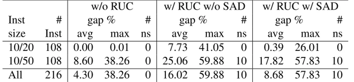
3.I Relation between the number of hosting and supporting trailers, as well as the corresponding construction costs. . . 32 3.II Comparing the solution quality for the DMCFLP without/with RUC
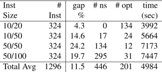
constraints as well as without/with SAD inequalities after one hour of computation time. . . 60 3.III Comparing the solution quality after one hour of computation time
using different solution approaches. . . 61 3.IV The average optimality gaps of optimal DMCFLP solutions in the
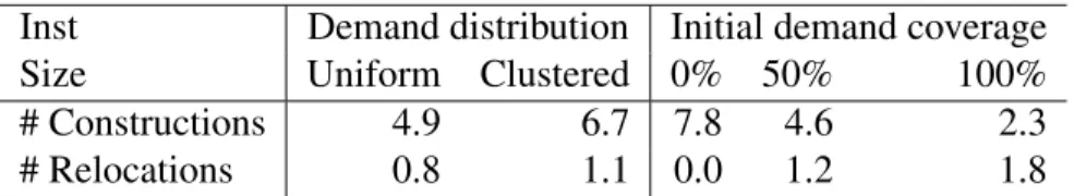
CSLP. . . 62 3.V The average number of constructed and relocated trailers within
near optimal CSLP solutions. . . 62 3.VI Results (ISall) with CSLPheur when camp relocation is allowed
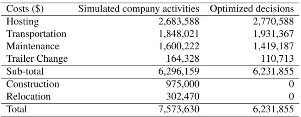
only once a year. . . 64 3.VII Cost distribution for the simulated company activities and the
op-timized solution. . . 68 3.VIII Cost distribution for optimal and heuristic demand allocation. . . 69 3.IX Cost distribution in the optimal solutions for both scenarios. . . . 71 3.X Usage of existing trailers and travel distances for the both scenarios. 72 4.I Average LP relaxation solution time and average integrality gaps
for all formulations. . . 96 4.II CPLEX branch-and-cut computation times (in seconds) for
in-stances solved to optimality by all formulations for each problem. 98 4.III CPLEX branch-and-cut optimality gaps for instances of the
DM-CFLP_CR not solved within 6hs. . . 99 4.IV CPLEX branch-and-cut optimality gaps for instances of the
xiii 4.V Computation times (in seconds) using CPLEX with default
set-tings for instances solved to optimality by all formulations for each problem. . . 101 4.VI Optimality gaps using CPLEX with default settings for instances
of the DMCFLP_CR not solved within 6hs. . . 102 4.VII Optimality gaps using CPLEX with default settings for instances
of the DMCFLP_ER not solved within 6hs. . . 102 4.VIII Impact of instance characteristics (transportation costs and demand
distribution) on the solution structure for the DMCFLP_CRER. . 106 4.IX Impact of number of time periods in problem instances (q = 10)
for the CRER-GMC formulation when using CPLEX with default settings. . . 107 5.I Comparison of different configurations for the Lagrangian based
heuristics for the four problems. . . 136 5.II Comparison of results for different parameters for the bundle method
with MIP based on Lagrangian solutions, applied to the DFLPG. . 138 5.III Comparison of CPLEX and Lagrangian based heuristics for the
DFLPG: average and maximum optimality gap when compared to the best known lower bound. . . 142 5.IV Comparison of CPLEX and Lagrangian based heuristics for the
DMCFLP_CR: average and maximum optimality gap when com-pared to the best known lower bound. . . 143 5.V Comparison of CPLEX and Lagrangian based heuristics for the
DMCFLP_ER: average and maximum optimality gap when com-pared to the best known lower bound. . . 144 5.VI Comparison of CPLEX and Lagrangian based heuristics for the
DMCFLP_CR_ER: average and maximum optimality gap when compared to the best known lower bound. . . 145
6.I Deviations of LP relaxation values from best known upper bounds for the two formulations of the DFLP_PC. . . 169 6.II CPLEX optimization, using the PC-2i and PC-GMC formulations
for the DFLP_PC. . . 171 6.III CPLEX results comparing the the two DFLP_PC formulations,
considering instances where both formulations found feasible so-lutions. . . 172 6.IV Results of the Lagrangian Heuristic for all 540 instances of the
DFLP_PC. . . 174 6.V Comparison of solution quality for CPLEX and the Lagrangian
heuristic for the DFLP_PC, considering instances where CPLEX found feasible solutions. . . 175 6.VI Deviations of LP relaxation values from best known upper bounds
of the RPC-2i and RPC-GMC formulations for the DFLP_RPC. . 177 6.VII CPLEX optimization, using the RPC-2i and RPC-GMC
formula-tions for the DFLP_RPC. . . 178 6.VIII CPLEX results comparing the two DFLP_RPC formulations,
con-sidering instances where both formulations found feasible solutions. 179 6.IX Comparison of solution quality for CPLEX and the Lagrangian
heuristic based on the relaxation of the demand constraints, con-sidering instances for the DFLP_RPC where CPLEX found feasi-ble solutions. . . 182 6.X Results of the Lagrangian Heuristic based on the relaxation of the
demand constraints for all 540 instances for the DFLP_RPC. . . . 183 6.XI Results of the Lagrangian Heuristic, relaxing demand and
reloca-tion linking constraints, for all 540 instances for the DFLP_RPC. . 184 6.XII Comparison of solution quality for CPLEX and the Lagrangian
heuristic, relaxing demand and relocation linking constraints, con-sidering instances for the DFLP_RPC where CPLEX found feasi-ble solutions. . . 186
xv 6.XIII Deviations of LP relaxation values from best known upper bounds
of the RPC-2i and RPC-GMC formulations for the DFLP_RPC with RUC constraints. . . 187 6.XIV CPLEX optimization, using the RPC-2i and RPC-GMC
formula-tions for the DFLP_RPC with RUC constraints. . . 189 6.XV CPLEX results comparing the two formulations for the DFLP_RPC
with RUC constraints, considering instances where both formula-tions found feasible soluformula-tions. . . 190 6.XVI Results for different configurations of the Lagrangian heuristic,
relaxing demand and relocation linking constraints, for all 540 in-stances for the DFLP_RPC with RUC constraints. . . 192 6.XVII Comparison of solution quality for CPLEX and the Lagrangian
heuristic, relaxing demand and relocation linking constraints, con-sidering instances for the DFLP_RPC with RUC constraints where CPLEX found feasible solutions. . . 193 A.I Computing times to solve the LP relaxation: direct arcs vs. hub
nodes. . . 222 A.II Computing time to solve problems: direct arcs vs. hub nodes. . . 223 B.I Model sizes for the formulations CR-GMC, CR-1I and CR-2I+. . 256 B.II Model sizes for the formulations ER-GMC, ER-1I and ER-2I. . . 257 B.III Model sizes for the formulations CRER-GMC and CRER-1I. . . . 258
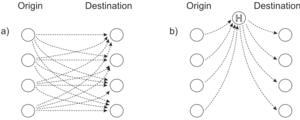
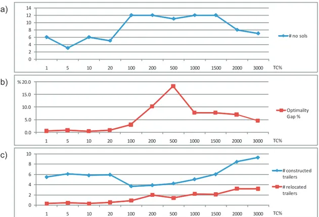
3.1 Example of facility relocation by the use of (a) direct arcs and (b) hub nodes. . . 32 3.2 Example of logging demands hosted at the same accommodation. 39 3.3 Network model to manage open and closed trailers at each location. 52 3.4 The impact of the transportation cost ratio on (a) the number of
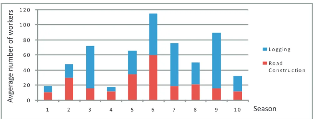
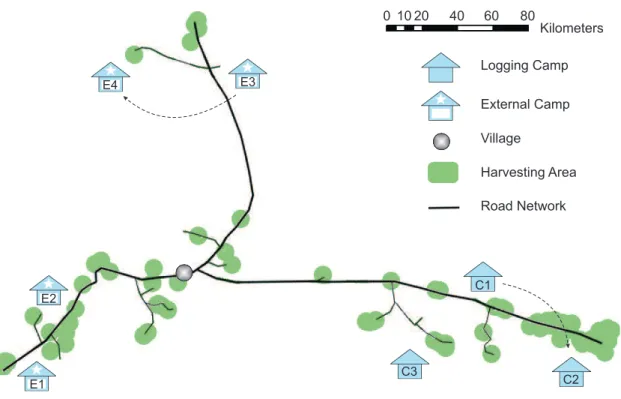
CSLP instances where no solutions have been found, (b) the aver-age optimality gaps and (c) the averaver-age number of constructed and relocated trailers in near optimal solutions. . . 63 3.5 Total demand (in average number of workers per day) throughout
all seasons. . . 65 3.6 Simplified illustration of the logging regions and the road network. 66 4.1 Capacity expansion/reduction by use of a single facility (a),
hori-zontal capacity blocks (b) and vertical capacity blocks (c). . . 81 4.2 Structure of optimal solutions: minimum, average and maximum
number of selected facility locations, as well as the average num-ber of open facilities per time period throughout the entire plan-ning horizon. . . 105 4.3 Structure of optimal solutions: average number of facility closings
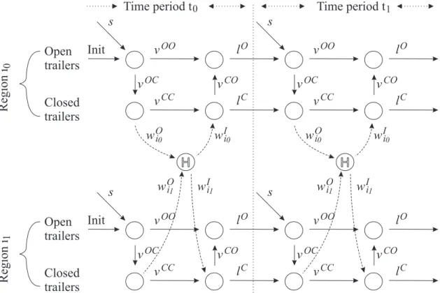
and reopenings, as well as capacity reductions and expansions. . . 105 6.1 Network model to manage partial facility closing and reopening
used in the PC-GMC and RPC-GMC models. Each node indicates the level of open and existing capacity. . . 154 A.1 Network flow structure for managing the number of open and closed
xvii A.2 Relative improvement of time to solve the LP relaxation for each
of the instances when hub node relocation is used instead of direct arcs. . . 222 B.1 Network flow to manage open and closed capacities at each facility
Combinatorial Optimization Problems
1I One index (normally refers to a formulation) 2I Two indices (normally refers to a formulation) 4I Four indices (normally refers to a formulation) CFLP Capacitated Facility Location Problem
(synonym: Capacitated Plant Location Problem) CSLP Camp Size and Location Problem
DFLP Dynamic Facility Location Problem
DFLPG Dynamic Facility Location Problem with Generalized Modular Capacities DFLP_PC Dynamic Facility Location Problem with Partial Facility Closing
DFLP_RPC Dynamic Facility Location Problem with Relocation and Partial Facility Closing FLP Facility Location Problem
GMC Generalized Modular Capacities
MCFLP Modular Capacitated Facility Location Problem MCKP Multiple-Choice Knapsack Problem
UFLP Uncapacitated Facility Location Problem (synonym: Simple Plant Location Problem)
Mathematical Programming B&B Branch-and-Bound B&C Branch-and-Cut
LP Linear Programming / Linear Program IP Integer Program
MIP Mixed-Integer Program
ADC Aggregated Demand Constraints RUC Round-Up Capacity Constraints
SAD Strengthened Aggregated Demand Constraints
xix Miscellaneous
LB Lower Bound UB Upper Bound
ACKNOWLEDGMENTS
First and foremost, I would like to express my sincerest gratitude to my supervisors, Professors Bernard Gendron and Jean-François Cordeau. I feel deeply fortunate and honored for the opportunity to work with them and would like to thank them for their confidence, support and advice both on research as well as on my career. Further, I would like to thank Professor Francisco Saldanha da Gama, the external examiner, for his valuable comments.
I am also thankful to the academic and technical staff of the Department of Computer Science and Operations Research of the Université de Montréal and the Interuniversity Research Centre on Enterprise Networks, Logistics and Transportation (CIRRELT).
I would like to thank Mathieu Blouin and Jean Favreau from FPInnovations, for their extensive collaboration on the industrial problem. Special thanks also to Ivan Contreras for his insights on Lagrangian relaxation, as well as to Antonio Frangioni and Enrico Gorgone for providing the implementation of the bundle method and advice on its us-age. I greatly appreciate the fruitful discussions with the many colleagues and friends at CIRRELT: Claudio, Fausto, Geraldine, Gerardo, Greg, Leandro, Marie-Eve, Paul, Thibaut, and many more. I also owe an important debt to Professor Marcus V. S. Poggi de Aragão, who introduced me to the field of operations research.
This list of acknowledgments would be incomplete without my deepest appreciation to my family, who always believed in me and fully accepted and supported my choice to live abroad. I am aware of all moments that I was not able to share with them. I am indebted to my wife Bérénice; strong, patient, and constantly supportive and loving. One cannot fail with someone like her by his side. Heartfelt thanks to my friends and life mentors Colette, Lorenzo, Michel et Nicolas, and many others in Montreal and around the world. Merci aux Québecois, pour leur accueil chaleureux, même aux jours froids.
Last, but not least, I also thank Calcul Québéc for providing excellent computing resources, as well as MITACS, the Natural Sciences and Engineering Research Council of Canada (NSERC) and the Fonds de recherche du Québec Nature et Technologies (FRQNT) for their financial support.
INTRODUCTION
The location of facilities is considered one of the most important decisions in logis-tics. Both the private and public sectors have shown a particular interest in the study of facility location, as they require to strategically locate warehouses, factories, fire sta-tions, schools, telecommunications hubs, and many others. Choosing the ideal location for a facility greatly depends on the application context and may take into considera-tion aspects that are as diverse as the distance to intermediate storage locaconsidera-tions or final customers, the accessibility of the facility terrain, the location’s susceptibility to natu-ral disasters, the accessibility and prices of necessary raw materials, the availability of qualified employees, or tax considerations and governmental initiatives. In most of the cases, the locations of facilities are strategic decisions that have a long lasting impact on the operational costs.
Given its economic importance, facility location has been of high interest for Op-erations Research (OR). In classical facility location, decisions aim to strike a balance between the fixed costs to supply capacity and the allocation costs to serve the demand. The latter often correspond to transportation costs to deliver products or provide services to customers. The vast literature on facility location problems can be traced back to as early as the beginning of the 20th century (Weber, 1929), when a single facility had to be placed to best serve the demand of customers. It has since been extended to a large variety of application contexts, with different objectives and different constraints. Hos-pitals have to be placed such that the maximum distance to the population is minimal, obnoxious facilities have to be placed as far as possible from the population, and budget constraints may limit the total investment. Among the many extensions that have been proposed, the most common ones include different commodity types for the customer demands, multiple periods in which customers may have different demands, as well as the choice of the facility size.
2 may solve these problems in polynomial time. However, many powerful solution meth-ods have been developed to solve these problems. With constant advances in information technology, as well as an increasing understanding of solution algorithms and the struc-ture of combinatorial optimization problems, the OR community has successfully solved increasingly complex and realistic problems.
Today’s challenges to advance facility location research may be divided into at least three categories, each of them holding opportunities to achieve significant impact in prac-tice. First, dynamic facility location takes into account the change in planning parame-ters over time. Uncertainty, in particular concerning the customer demands, may require a robust choice of the facility location. Population shifts, evolving market trends and changes of other environmental factors often require adjustments reaching from facili-ties to the entire supply chain. These adjustments often concern the decisions of where and when to provide capacity to best satisfy the customer demands. Another impor-tant challenge is to represent a problem in a more realistic manner. Typically, this can be done by ensuring that the individual problem constraints are modeled realistically and by representing the cost structure of the problem on a sufficiently detailed level. Economies of scale have often been considered on levels such as the facility’s construction, main-tenance and production costs. They may also be found on other levels such as the costs to deliver the products to the customers. Finally, integrated planning problems aim at acknowledging the interaction between several planning problems and try to solve them simultaneously, such as in location-routing problems and in integrated facility location with network design. Taking these aspects into consideration when designing facility location problems holds a valuable opportunity to represent the problems in a more real-istic manner and therefore provide more tools for supporting decision making processes. However, even today, modeling and solving such problems remains a challenge.
The objective of this thesis is to contribute with models and algorithms to solve dy-namic facility location problems, in particular responding to the first two of the above mentioned challenges. This thesis focuses on multi-period facility location problems in which the planning parameters may be subject to significant changes over time. Fa-cilities adapt to the new environment by adjusting the available capacity at each of the
locations. The proposed models also take into consideration a very detailed level of the cost structure, enabling a more realistic representation of the problems. The work on these problems has been inspired by an industrial collaboration with FPInnovations, one of the world’s largest private, non-profit research centers working in forest research. The project aims at providing a decision support tool for a Canadian logging company that has to locate logging camps to host the workers involved in forestry operations. Although it is an extension of classical multi-period facility location problems, this problem does not only possess very specific constraints, but also a very detailed cost structure. As solving these problems exactly by the use of generic mixed-integer programming (MIP) solvers is only successful for small problem instances, we develop heuristics based on Lagrangian relaxation to provide high quality solutions in short computation times, even for large-scale instances.
The remainder of this thesis is organized as follows. In Chapter 2, we review the lit-erature for facility location problems. Given the vast amount of litlit-erature that has been produced in this domain in the last decades, we focus on the classical Capacitated Fa-cility Location Problem (CFLP)and its variants. In the first part, the CFLP is discussed within the context of location analysis. A classification scheme is provided to guide the discussion on variants and extensions of the classical problem. In particular, we discuss the choice of the facility size, multiple commodities and dynamic adjustment of capaci-ties. The second part of the chapter concerns solution methods that have been proposed for these problems. We then draw conclusions concerning the existing literature.
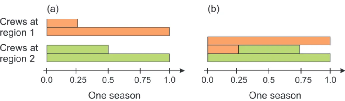
Chapter 3 introduces an industrial application that can be found in the Canadian forestry sector. The problem is referred to as the Camp Size and Location Problem (CSLP)and investigates where to locate and relocate logging camps to host workers in-volved in the forest operations. This problem can be abstracted to a multi-period facility location problem with multiple commodities that allows for the capacity expansion at facilities, as well as the relocation of facilities from one location to another. This prob-lem contributes to the literature by extending existing probprob-lems in several ways. First, facilities may be partially closed during certain time periods. Second, the problem pos-sesses particular capacity constraints in which the total demand allocated to each facility
4 is rounded to the next highest integer value. Finally, the problem has a detailed cost structure for capacity changes, i.e., capacity expansion, as well as for the closing and reopening of capacities. A MIP model based on capacity flows, as well as new valid inequalities for the particular capacity constraints, are presented. All individual prob-lem characteristics are taken into account, while the detailed cost structure for capacity changes is approximated. It is shown how the problem can be tackled more efficiently by solving a simplified version of the problem and using its solutions to warm start the MIP solver. Two case studies exemplify the usefulness of the model in practice.
In Chapter 4, we then introduce a very general dynamic facility location problem, referred to as the Dynamic Facility Location Problem with Generalized Modular Capac-ities (DFLPG). The problem is characterized by modular capacity changes subject to a detailed cost structure. Due to its generality, the proposed MIP model unifies several existing problems found in the literature. This is illustrated by means of three special cases: the problem with facility closing and reopening, the problem with capacity ex-pansion and reduction, and the combination of the two. The cost structure used in the DFLPG is based on a matrix describing the costs for capacity changes between all pairs of capacity levels, capable to represent complicated cost structures such as the one found in the CSLP. We are not aware of any other work dealing with facility location with a similar level of detail in the cost structure. We analyze the linear programming (LP) relaxation bound obtained by our model, showing that it is at least as strong as the LP relaxation bound of existing specialized formulations. Furthermore, we perform compu-tational studies on a large set of randomly generated instances with up to 100 candidate facility locations (each with up to 10 capacity levels), 1000 customers and 14 time peri-ods. The results show that our model, when solved with a state-of-the-art MIP solver, can obtain optimal solutions in significantly shorter computation times than the specialized formulations for the three special cases.
Chapter 5 is devoted to the solution of a DFLPG extension in which customers have demands for different commodities. We propose Lagrangian based heuristics that find good quality solutions in reasonable computing times. Two methods are used to solve the Lagrangian dual: a subgradient method and a bundle method. After this process, a
second optimization step is used to improve the solution quality. This step consists of solving a restricted MIP model, taking into consideration only decisions that have been part of a significant number of the previous Lagrangian solutions. Computational results are given for large instances with up to 250 candidate facility locations and 1000 cus-tomers. The results are stable even for large instances, for which general-purpose MIP solvers either consume too much memory or do not solve the problem in reasonable time. To the best of our knowledge, this work is the first to present a Lagrangian relaxation approach to solve large-scale instances of a multi-period facility location problem of this nature, i.e., including modular capacity adjustments and multiple commodity types.
We then close the loop in Chapter 6 by demonstrating how to extend the Lagrangian heuristics to the case of the CSLP or similar problem variants. An alternative formu-lation, based on the same modeling technique used to model the DFLPG, is presented. Even though the size of this formulation is too large to be handled by generic MIP solvers, the subproblems are of quite reasonable size when decomposed by Lagrangian relaxation. The algorithm from the previous chapter is modified to additionally account for the partial closing and reopening of facilities, the relocation of facilities, and the par-ticular capacity constraints defined in the CSLP. Two different relaxations are presented, each relaxing different sets of constraints. Computational results show the benefit of the Lagrangian heuristics when compared to the use of generic MIP solvers.
Finally, Chapter 7 summarizes the contributions of this thesis and discusses potential future research directions.
CHAPTER 2
LITERATURE REVIEW
In this chapter, we review the literature relevant to the facility location problems we study in this thesis. Section 2.1 introduces classical facility location problems, their variants and extensions, as well as their applications. Section 2.2 focuses on solution methods for the previously introduced problems. Finally, in Section 2.3, we discuss the importance of the existing literature for the work presented in this thesis.
2.1 An Overview of Facility Location Problems and Applications
This section introduces facility location in the broader context of location analysis and reviews classical facility location problems and their variants and extensions. Then, the most common applications are discussed.
2.1.1 Facility Location in the Context of Location Analysis
Location Analysis is concerned with identifying the optimal locations subject to con-text related constraints. Often, the former are referred to as the locations of facilities, placed to efficiently serve the demand of customers. Literature on location problems can be traced back to as early as 1909 in a book by Alfred Weber, first published in German and later translated into English (Weber, 1929). This work considered the location of a production facility to minimize the total sum of distances to a set of customers. The field of location analysis mostly grew during the 1960’s (Smith et al., 2009) and discrete location problems are nowadays a large branch of combinatorial optimization. Many schemes have been proposed to classify location models (Hamacher and Nickel, 1998). One of the basic criteria categorizes the problems into analytic, continuous, network, and discrete location models (Daskin, 2008; Revelle et al., 2008). Analytic models are the simplest form of location problems and are based on simplifying assumptions re-garding their constraints and their objective function, such as the cost structure. They
are typically solved analytically, using calculus or other techniques. Continuous loca-tion modelstypically assume a discrete set of demand points, while the locations for the facilities are chosen in the continuous space. A well known example for this class of location models is the above mentioned Weber problem. Network models assume that facilities can be placed on the nodes or links of a specified network, while demands are typically placed on the nodes. Discrete location models form a special case of network models where demands are given by a discrete set of nodes and facilities may be located on a discrete set of candidate locations.
The category of discrete location models has constantly evolved in the last decades and offers a rich literature on different problems and solution methods to solve them. It can be further classified (Daskin, 2008; Revelle et al., 2008) into median and plant location problems, as well as center and covering problems. A similar classification has also been proposed by Revelle and Eiselt (2005). The development of location analysis from its early beginning and today’s most important applications are also reviewed by Smith et al. (2009). Covering problems investigate the minimum number of facilities necessary to guarantee a certain maximum distance between the customers and their assigned facilities. Center problems aim at minimizing the maximum distance between the customers and facilities to which they are allocated.
The p-median problem is the simplest problem of the first category of discrete lo-cation models. It is known to be NP-hard (Kariv and Hakimi, 1979a,b) and aims at finding the optimal locations for p facilities such that the total average weighted dis-tance between the customers and their assigned facilities is minimal. The essence of this problem, i.e., serving customer demands at minimum cost, is preserved in most of the problem extensions. Typically known as plant or facility location problems, these vari-ants generalize the p-median problem by introducing heterogeneous construction costs and a flexible choice of the number of facilities p.
The authors cited above also comment on other classes of discrete location mod-els. Competitive location problems (Eiselt et al., 1993) deal with facility location in the presence of competitors. Locations have to be chosen such that the market share is maximized. Hub location problems (O’Kelly, 1986; Contreras et al., 2011b; Campbell
8 and O’Kelly, 2012) locate transportation hubs according to a given flow from origins to destinations. While facilities are usually located as close as possible to their customers, some problems may aim at the opposite. For example, undesirable (or obnoxious) facil-ities (Berman and Wang, 2008) may impose health risk to the population and therefore have to be located in a sufficient distance. The combination of different planning prob-lems has also been considered, such as the Location-Routing problem (Contardo et al., 2013; Prodhon and Prins, 2014) and integrated logistics network design (Cordeau et al., 2006).
In the following, we will focus on facility location problems and their main variants proposed in the literature.
2.1.2 Capacitated Facility Location
In the following, we review classical capacitated facility location problems. We then discuss literature surveys and classical problem extensions. A classification scheme is provided that guides the discussion on different problem characteristics.
2.1.2.1 The Capacitated Facility Location Problem
As has been mentioned in the previous section, facility location problems are impor-tant extensions of the classical p-median problem. The Uncapacitated Facility Location Problem (UFLP), also known as the Simple Plant Location Problem, aims at selecting a number of facility locations from a discrete set of candidate locations j ∈ J, considering the construction costs fj for each of the facilities. Customer demands di are given for
each customer i defined by a discrete set I. These demands have to be satisfied at min-imum cost, also taking into consideration the aggregated production and transportation costs ci j to serve one demand unit of customer i by facility j. Clearly, the capacitated
case, referred to as the Capacitated Facility Location Problem (CFLP), is a more re-alistic model, as production capacities are usually limited. It is known to be strongly NP-hard (Cornuéjols and Sridharan, 1991). Here, the binary variables yj take value 1
vari-ables xi j represent the fraction of the demand from customer i that is served by facility
j. Using this notation, the CFLP can be formulated as follows (Sridharan, 1995):
(CFLP) min
∑
j∈J fjyj+∑
i∈I∑
j∈J ci jdixi j (2.1) s.t.∑
j∈J xi j = 1 ∀i ∈ I (2.2)∑
i∈I dixi j≤ ujyj ∀ j ∈ J (2.3) 0 ≤ xi j≤ 1 ∀i ∈ I, ∀ j ∈ J (2.4) yj∈ {0, 1} ∀ j ∈ J. (2.5)The problem minimizes the total cost composed by facility construction and demand allocation. Equalities (2.2) ensure that all customer demands are met. Constraints (2.3) are the capacity constraints at the facilities.
Note that the presented model allows the demand of a customer to be met by different facilities. Certain variants require that each customer is allocated to a single facility, defining xi j as binary, also referred to as single-sourcing.
2.1.2.2 Literature Surveys and Problem Classification
The facility location community benefits from a rich and diverse literature dating back to the early 19th century (Krzyzanowski, 1927). The diversity, importance and maturity of the field has been confirmed by many recent literature surveys (Hamacher and Nickel, 1998; Klose and Drexl, 2005; Melo et al., 2009a; Revelle and Eiselt, 2005; Revelle et al., 2008; Smith et al., 2009; Zanjirani Farahani and Hekmatfar, 2009). Sev-eral classification schemes have been proposed to point out similarities and differences between the existing models. Melo et al. (2009a) focuses on criteria in the context of Supply Chain Management, whereas Klose and Drexl (2005) specify a classification for facility location problems. One may slightly extend their classification scheme and characterize facility location problems by the following properties:
10 – Metric of the underlying network. Based on the shape or topology of the trans-portation network, the distances and costs may be based on Euclidean distances or other more complex structures.
– Type of the objective function. The problem may minimize the total sum of distances or the maximum distance between the customers and the facilities they are assigned to.
– Facility capacities. If facilities possess capacities, they may have fixed or flexi-ble capacities. Capacity modifications may be continuous or chosen according to predefined capacity levels.
– Single-facility vs. multi-facility. Each location may either possess a single facil-ity or several facilities, independent or interacting.
– Single-echelon vs. multi-echelon. In multi-echelon models, the commodity flow may pass trough several echelons, such as facilities, warehouses, depots, and fi-nally the customer. Reverse flows may be allowed. A direct flow from facilities to customers corresponds to a single-echelon model.
– Single-commodity vs. multi-commodity. Customers may have demands for dif-ferent commodities. Facilities may produce only a certain subset and a certain quantity of commodities.
– Single-period vs. multi-period. Models with a single time period rarely cor-respond to realistic applications. Multiple time periods may involve independent demands and costs for each of the time periods, as well as the opportunity to adjust the locations and capacities of facilities along the planning horizon.
– Deterministic vs. uncertain. In practice, certain input data may be subject to uncertainty. Even when data, such as customer demands, can be well predicted, the real values will most probably differ from the predicted value.
– Single-source vs. multi-source. Customer demands are either met by a single facility or by different facilities.
Some of these characteristics are similar for most of the works found in facility lo-cation literature. For example, the majority of the proposed models aims at minimizing the total costs to serve the customers. Only few assume a fixed budget (e.g., Wang
et al., 2003; Sonmez and Lim, 2012). In a similar manner, most of the works assume that customer demands may be served by different facilities (multi-source), while only a few constrain the customer demands to single-sourcing (e.g., Agar and Salhi, 1998; Holmberg et al., 1999; Albareda-Sambola et al., 2009). Some other characteristics have evolved to individual classes of facility location problems, each of them offering a tai-lored literature on how to model and solve them. In the following, we use the above classification criteria to guide the discussion on the existing facility location literature. We emphasize problem characteristics that are found in the CSLP (see Section 3), the industrial application that has inspired large parts of the research presented in this thesis. Multi-period problem variants are discussed in Section 2.1.3.
2.1.2.3 Choice of the Facility Size and Cost Structure
Given that in most of the application contexts resources are finite, the majority of the proposed facility location models impose capacities on the facilities. In an effort to represent cost structures realistically, many researchers acknowledged the importance of economies of scale (Holmberg and Ling, 1997; Agar and Salhi, 1998; Correia and Captivo, 2003; Correia et al., 2010), i.e., the larger the facility, the cheaper the unit price in terms of facility construction and commodity production. Similarly, some applica-tions involve cost structures that imply inverse economies of scale (Harkness, 2003), where the unit price increases as the facility gets larger. To enable the representation of such cost structures, many models decide not only for the location of facilities, but also for their total capacity instead of assuming a fixed capacity. Problems that involve the choice of the facility size are known under different names, such as the Dynamic Ca-pacitated Plant Location Problem(Shulman, 1991) in the multi-period context, and the Multi-capacitated Plant Location Problem(Agar and Salhi, 1998) or Modular Capaci-tated Location Problem(Correia and Captivo, 2003) in the single-period context. Early works with a choice of capacities include those of Lee (1991, 1993a,b), Shulman (1991) and Sridharan (1991). In these works, the choice of the capacity level is modeled using an additional variable index, resulting in a facility variable of the form yj`, ` ∈ L, where
ca-12 pacity. This intuitive modeling technique has been adapted by several other researchers (Sankaran and Raghavan, 1997).
An alternative modeling technique has been presented in Holmberg (1994) and Holm-berg and Ling (1997). The authors use an incremental approach to model staircase functions, where all variables up to the chosen capacity level are active. Similar ap-proaches have since been adapted for more complex location problems (Correia and Captivo, 2003; Gouveia and Saldanha da Gama, 2006). While most of these works con-sider economies of scales in the construction costs, Correia and Captivo (2003) also represent economies of scale in the total amount of produced commodities. The authors separate the decision of the production level from the demand allocation variables x by using additional binary variables of the form wj`to indicate the total amount produced
at facility j working at capacity level `.
Most of the works discussed above propose models where a single facility can be located at each location. However, the total capacity available at a site may also be configured by choosing more than one facility at the same location (Wu et al., 2006). Some of these works involving multiple time periods are discussed further below in the context of capacity expansion and reduction over time.
2.1.2.4 Multiple Commodities
Customers may have demands for several distinct commodities and facilities may produce different commodity types. Multiple commodities have become a common ex-tension to classical facility location problems, in particular since they do not further complicate the structure of the model. Models can be distinguished between those that allocate a separate production capacity for each commodity (Canel et al., 2001; Geof-frion and Graves, 1974; Lee, 1991; Warszawski, 1973; Pirkul and Jayaraman, 1998) and those that assume that the production capacity of a facility covers all commodity types at once (Melo et al., 2006). The constraint type depends on the application context. The first type is often used to indicate different technologies or facility types that enable the production of a certain commodity type (Lee, 1991; Pirkul and Jayaraman, 1998). It is modeled by using separate capacity constraints for each commodity. In the second type,
the same capacity constraint is used for all commodities and sums up the entire demand allocation.
New research directions also explore the interaction between facilities that produce different commodities, where one facility may benefit from the by-product of another nearby facility (Xie and Ouyang, 2013).
2.1.2.5 Other Generalizations and Variants
Another important class of facility location problems takes into account stochastic and probabilistic elements (Snyder, 2006). In these problems, the input data is not deter-ministic, but subject to uncertainty. Uncertainty has mostly been assumed to concern the customer demands (Schütz et al., 2008). However, it may also concern other input data such as the traveling times on the transportation network (Berman and LeBlanc, 1984).
Multi-echelon facility location (Zanjirani Farahani et al., 2014), also referred to as multi-level, multi-layer or multi-stage facility location, assumes that the product passes several layers before it reaches its final destination. These kinds of models are very common to model supply chains (Thomas and Griffin, 1996), also known as production-distribution systems (Thanh et al., 2008), where the commodities may be produced in facilities, stored in warehouses and sent to stores or customers. In many applications, there is a natural hierarchy given that the product moves downstream in the supply chain (Gendron and Semet, 2009; Gendron et al., 2011, 2013). In contrast, problems in which the network of commodity flow may contain cycles are said to involve reverse flows and fall in the area of reverse logistics (Alumur et al., 2012).
The majority of works discussed in this thesis have one simple and common objec-tive: the minimization of costs. However, many other objectives are possible. Multi-objective problems aim at combining several, often conflicting, Multi-objectives. A very typ-ical example is the combination of traditional economic objectives and the reduction of environmental impact. Given that the public becomes more aware of environmental issues, both the governmental and private sectors will most likely analyze how green their supply chain and production process are (Dekker et al., 2012), aiming at the reduc-tion of their carbon footprint and the opportunities to recycle. These are opportunities
14 to explore reverse logistics supply chains as discussed above, but also to combine the traditional economic objective with environmental goals and their impacts (e.g., Hugo and Pistikopoulos, 2005; Harris et al., 2014). Other facility location problems involving multiple objectives include the work of Melachrinoudis (2000), which additionally aims at minimizing the time to access the product.
2.1.3 Dynamic Facility Location
The majority of facility location models are applied to strategic long-term planning. However, customer demands, as well as the prices for production, transportation and commodities tend to change over time. Multi-period models aim at coping with these challenges by defining independent demands and costs for each time period. Early works in the domain of dynamic facility location were initiated by authors such as Ballou (1968), Wesolowsky (1973), Wesolowsky and Truscott (1975) and Sweeney and Tatham (1976). A few authors used the term dynamic in a broader context (Arabani and Zanji-rani Farahani, 2011; ZanjiZanji-rani Farahani and Hekmatfar, 2009), also including stochastic aspects. However, the majority of the literature limited the use of the term to the con-text of multi-period problems. From the modeling viewpoint, the temporal aspect is usually captured by an additional variable index t. While a few models represent the available capacity by an additional flow variable zjt ∈ R+, most of the works
incorpo-rate modular capacities, using binary variables of type yj`t, where ` is either a capacity
level or a facility type linked to a fixed amount of capacity. While the optimal timing of a facility construction, as well as its initial capacity are important decisions (e.g., Shulman, 1991), it has often been found beneficial to adjust capacities at later time pe-riods to better respond to changing demand and market conditions (Owen and Daskin, 1998). Mathematical models that include such features have been applied in both the private and the public sectors to determine locations and capacities for production facil-ities, entire supply chains (Melo et al., 2006), telecommunications networks (Chardaire et al., 1996), schools (Antunes and Peeters, 2001), ambulances (Brotcorne et al., 2003), emergency services (Hochbaum, 1998) and many more, responding to population shifts and other environmental factors. Several surveys (Owen and Daskin, 1998; Arabani and
Zanjirani Farahani, 2011; Zanjirani Farahani and Hekmatfar, 2009) reviewed the grow-ing literature on dynamic facility location problems, which suggested different ways to adjust capacities throughout a given planning horizon:
– The construction of a facility at a certain time period.
– The expansion or reduction of capacity at an existing facility.
– The temporary closing of a facility and reopening at a later time period. – The relocation of capacity from one location to another.
The timing of facility construction is part of most of the multi-period facility location problems. We now review the existing literature for the other three features.
2.1.3.1 Capacity Expansion and Reduction
When customer demands of certain regions permanently change and are not likely to return to their previous levels, it may be beneficial to add or reduce (or even permanently shut down) production capacities at an existing facility to permanently adjust to the new conditions.
Luss (1982) discusses modeling techniques for capacity expansion. He points out that the total capacity available at a location may either be provided by a single facility or be composed by several coexisting facilities. The first category includes models that allow one facility at a location that increases or decreases the available capacity over time (Jacobsen, 1990; Canel et al., 2001; Antunes and Peeters, 2001; Melo et al., 2006; Behmardi and Lee, 2008). These models typically use flow variables of type zjt ∈ R+
and manage the expansion (sjt ∈ R+ variables) or reduction (rjt ∈ R+ variables) of
ca-pacity by using flow conservation constraints similar to the following:
zjt = zj(t−1)+ sjt− rjt ∀i ∈ I , ∀t ∈ T (2.6)
Models in the second category commonly use integer variables to indicate the num-ber of existing facilities at a location. When the problem allows for capacity expansion, but not reduction, the total capacity can also be composed of several binary variables, one for each constructed facility or expanded capacity (Shulman, 1991; Troncoso and
16 Garrido, 2005). This modeling technique can also be found in other classes of loca-tion problems, such as variants of the Capacitated Concentrator Problem (Gouveia and Saldanha da Gama, 2006; Gourdin and Klopfenstein, 2008; Correia et al., 2010).
When the problem involves both capacity expansion and reduction, an alternative modeling technique (Dias et al., 2007) can be used involving binary variables of type yj`t1t2 to indicate that a capacity of size ` is added for a period defined by the interval [t1,t2]. The total capacity available at a location and time period is then computed by the
sum of all facilities (capacity blocks) available at that time period, enabling a flexible expansion and reduction of capacity along time. The two different categories, using flow variables and capacity block variables, are illustrated in Figure 4.1. We refer to Section 4.3 for a detailed discussion of these modeling techniques.
Next to classical capacity expansion and reduction, several special cases with in-dividual restrictions have been presented. In the work of Antunes and Peeters (2001), facilities may either expand or decrease their capacities throughout the planning hori-zon, but not both. We refer to the book chapter of Jacobsen (1990) for more references to works that consider capacity expansion.
2.1.3.2 Temporary Facility Closing and Reopening
In some situations, it may be beneficial to temporarily close a facility, for example to avoid high maintenance costs. This may be appropriate when demand temporarily decreases, but is likely to return to its previous level afterwards. While, in practice, it may be possible to close only parts of a facility, previous studies focused on the tem-porary closing of entire facilities. Among the suggested models, certain are limited to a single closing and reopening of each facility, whereas others allow repeated closing and reopening throughout the planning horizon. The uncapacitated facility location prob-lem presented by Van Roy and Erlenkotter (1982), as well as the supply chain model of Hinojosa et al. (2008), allow one-time opening or closing of facilities: new facilities can be opened once and existing facilities can be closed once. Chardaire et al. (1996) and Canel et al. (2001) propose formulations for opening and closing facilities more than once. The former installs and removes terminals in telecommunications networks
to adapt to changes in data traffic and costs along time. The authors of both works use binary variables of type yjt to indicate whether a facility is open or closed during a
cer-tain period. A closing or reopening is then indicated by a quadratic term yjt(1 − yjt) in
the objective function. A linear formulation for a simplified variant of this problem with fixed capacity levels has been proposed by Dias et al. (2006).
The works cited above interpret facility closing either as temporary (i.e., the facility still exists, but its capacities are temporarily unavailable) or permanent (a facility is shut down). In most cases, maintenance costs for temporarily closed facilities are low and can therefore be ignored in the model. Most of the existing formulations therefore do not explicitly distinguish temporary and permanent facility closing. Furthermore, permanent facility closing may also be seen as a special case of capacity reduction.
2.1.3.3 Facility Relocation
In certain contexts, the relocation of existing capacity from one location to another may be a possibility to shift capacity closer to the demand points. Wesolowsky and Truscott (1975) have been one of the first to consider simple relocation of facilities. The authors use flow conservation constraints similar to (2.6), but with binary variables (instead of flow variables) to indicate whether a facility is available or not. That is, instead of variables representing capacity expansion and reduction, the model contains binary variables to represent the relocation from or to the location.
The relocation of facilities has since been considered by several researchers. Min and Melachrinoudis (1999) document a case study for a company that relocates warehouses and Melachrinoudis (2000) provides an appropriate model. Brotcorne et al. (2003) re-view location-relocation models for ambulances for deterministic and probabilistic sce-narios. Melo et al. (2006) and Melo et al. (2009b) provide an extensive modeling frame-work for modeling generic multi-level supply chain netframe-work structures. Their model is based on flow conservation constraints and focuses on gradual relocation of existing ca-pacity. The authors also show how to link binary variables to indicate the facility type, as well as the origin and destination for the relocated facility. However, it can be noted that most of the other works ignore the distance the facilities are relocated and therefore
18 allocate equal costs to all facility relocations.
Often, the closing of a facility at one location and opening at another location has also been interpreted as a facility relocation, which has been considered under the constraints of a global budget (Wang et al., 2003) and under demand uncertainty (Lim and Sonmez, 2013).
Relocation models have also been proposed under more restricted conditions. Amiri-Aref et al. (2011) present a non-linear mixed-integer formulation to relocate emergency maintenance rooms given that the transit availability for certain regions are subject to uncertainty. Zanjirani Farahani et al. (2008) locate and relocate a single facility under the condition that costs vary according to a continuous weight function. Albareda-Sambola et al. (2009) introduce a problem in which facilities must select a certain number of customers. Once served, customers have to be served in all subsequent periods.
2.1.4 Applications
Facility location problems have been applied in many different contexts. In the pri-vate sector, facility location models most often concern the locations of manufactur-ing and distribution systems (Min and Melachrinoudis, 1999; Broek et al., 2006) and telecommunications networks (Chardaire et al., 1996). Location models have also been often used in the public sector to locate schools (Antunes and Peeters, 2001), hospitals (Vahidnia et al., 2009) or for military logistics (Gue, 2003; Ghanmi, 2010). Many more references can be found in surveys such as those by Arabani and Zanjirani Farahani (2011) and Melo et al. (2009a)
The forestry sector has also been an active user of facility location and supply chain optimization models. Transportation in the forestry domain accounts for a large part of the total operational costs (Audy et al., 2012), reported to be 25-35% in Southern USA, more than 35% in Canada and more than 45% in Chile. Naturally, studies have been strongly contributed from countries with significant log export, such as it is the case in Canada (Haartveit et al., 2004; Vila et al., 2006), Chile (Epstein et al., 1999; Troncoso and Garrido, 2005) and the Scandinavian countries (Rönnqvist, 2003; Bredström et al., 2004; Carlsson and Rönnqvist, 2005). Chan et al. (2009) provide a facility location
model to place satellite yards. A comprehensive introduction is provided by D’Amours et al. (2008), also providing further references. We also refer to the work of Vahid and Maness (2010) who have recently reviewed and classified supply chain literature for the forestry sector.
2.2 Solution Methods
We now review solution methods that have commonly been used to solve facility lo-cation problems. Solution methods for optimization problems can be distinguished into two broad classes: exact and heuristic methods. Exact methods solve the problem to optimality, given that sufficient time and memory is available. If, for some reason, the problem is not solved to optimality, exact methods can provide bounds on the optimal solution value. As has been seen in the previous section, it has become common prac-tice to model location problems as MIP models. It is equally common that generic MIP solvers, usually based on elaborate exact methods, are used to solve these models. How-ever, even though generic solvers and information technology constantly advance, OR practitioners try to model real world applications more and more realistically and solve instances as large as possible. Given the complexity of the resulting models, it is often not possible to solve them exactly. Heuristics aim at providing high quality solutions in short computing times even for large problems. Several surveys (Sridharan, 1995; Arabani and Zanjirani Farahani, 2011; Melo et al., 2009a) review some of the many ex-act and heuristic solution methods that have been proposed. Some of the algorithmic advances have been implemented to improve the performance of generic solvers, while other approaches require to be customized to each problem and therefore form a method-ological category by themselves. In the following, we will review the literature for the methods that have been most successful and popular to solve facility location problems.
2.2.1 Exact Methods: Polyhedral Approaches
Most of the facility location problems have been modeled as linear MIP models. Many of them (Sankaran and Raghavan, 1997; Melachrinoudis, 2000; Melo et al., 2006;
20 Wilhelm et al., 2013) have been solved to optimality within reasonable time by general-purpose solvers. These solvers, such as IBM ILOG CPLEX (IBM, 2010), the Gurobi Optimizer (Gurobi Optimization, Inc., 2014) and COIN-OR (2014), aim at providing an efficient framework to solve generic, in particular linear MIP models, to optimality. To prove optimality, generic MIP solvers are typically based on some sort of Branch-and-Bound (B&B)algorithm. Certain binary variables are fixed to one of their feasible values, forming a branch in the B&B tree. Typically, the LP relaxation then provides a lower bound (in the case of a minimization problem) on the optimal integer solution value that may be found in the corresponding branch. Integer feasible solutions are typically used to provide an upper bound on the optimal integer solution. As B&B algorithms rely on the concept of complete enumeration of the decision tree, their performance crucially depends on their ability to prune branches that are not promising to lead to an improved feasible solution, i.e., when the lower bound of a branch is not smaller than the best upper bound available. Therefore, pruning tends to be more successful when the integrality gap of the model (i.e., the relative gap between the optimal integer solution value and the LP relaxation solution value) is small.
A valid inequality is an inequality that is satisfied by all feasible integer solutions of the MIP model. Cuts are valid inequalities that are not part of the current problem formulation and are commonly used to approximate the convex hull of the set of integer feasible solutions. The tighter the formulation is, the smaller the integrality gap tends to be. Branch-and-Cut (B&C) algorithms are B&B algorithms that may add cuts at each node in the tree. B&C algorithms provide the foundation for many generic solvers. To derive effective cuts, the CFLP has been extensively studied in terms of its polyhedral structure. Reference works include those by Leung and Magnanti (1989) and Aardal et al. (1995). Aardal (1998b) strengthens the formulation by introducing redundant vari-ables to derive valid inequalities afterwards. Cutting Plane algorithms for facility loca-tion problems are presented by Aardal (1998a) and Avella and Boccia (2007). A few authors also presented customized B&B algorithms (Görtz and Klose, 2012).
As many of the developed cuts are based on sets that are extremely large, one cannot add all cuts to the model. Separation algorithms (Aardal, 1998a) are necessary to identify
cuts that actually improve the LP relaxation bound. However, a few valid inequalities have been developed whose number is polynomial in the size of the input data and suf-ficiently small to be added a priori to the model. Some of these cuts are quite effective when added to the model and can be used in combination with other solution approaches to facilitate the solution of the problem. The Strong Inequalities (Van Roy, 1986), also referred to as the Strong Linking Constraints (Gendron and Crainic, 1994), have been shown to be very effective to increase the value of the facility opening decisions in the LP relaxation. For the CFLP as given by (2.1 - 2.5), they are defined as follows:
xi j≤ yj ∀i ∈ I, ∀ j ∈ J. (2.7)
Another important class of valid inequalities are the Aggregated Demand Constraints (ADC)(Cornuéjols and Sridharan, 1991):
∑
j∈Jyj≤
∑
i∈Idi. (2.8)
Even though they are redundant to the LP relaxation, they often enable generic MIP solvers to derive further cuts.
2.2.2 Mathematical Decomposition
Methods based on mathematical decomposition exploit the structure of linear pro-grams to decompose them into smaller and easier subproblems. Even though, for most of these methods, convergence is formally provided, in practice it is often slow or not achievable. Some of these techniques, in particular those based on Lagrangian relax-ation, are therefore often used to solve the problem heuristically. In the following, Ben-ders decomposition, Lagrangian relaxation and cross decomposition will be discussed in the scope of facility location problems.