ÉCOLE DE TECHNOLOGIE SUPÉRIEURE UNIVERSITÉ DU QUÉBEC
MANUSCRIPT-BASED THESIS PRESENTED TO ÉCOLE DE TECHNOLOGIE SUPÉRIEURE
IN PARTIAL FULFILLMENT OF THE REQUIREMENTS FOR THE DEGREE OF DOCTOR OF PHILOSOPHY
Ph.D.
BY
Oliviu ŞUGAR GABOR
VALIDATION OF MORPHING WING METHODOLOGIES ON AN UNMANNED AERIAL SYSTEM AND A WIND TUNNEL TECHNOLOGY DEMONSTRATOR
MONTREAL, 18TH OF DECEMBER 2015 © Copyright 2015 reserved by Oliviu Şugar Gabor
© Copyright
Reproduction, saving or sharing of the content of this document, in whole or in part, is prohibited. A reader who wishes to print this document or save it on any medium must first obtain the author’s permission.
BOARD OF EXAMINERS
THIS THESIS HAS BEEN EVALUATED BY THE FOLLOWING BOARD OF EXAMINERS
Dr. Ruxandra Mihaela Botez, Thesis Supervisor
Department of Automated Production Engineering at École de Technologie Supérieure
Dr. Philippe Bocher, Chair, Board of Examiners
Department of Mechanical Engineering at École de Technologie Supérieure
Dr. Guy Gauthier, Member of the Jury
Department of Automated Production Engineering at École de Technologie Supérieure
Dr. Marius Paraschivoiu, External Evaluator
Department of Mechanical and Industrial Engineering, Concordia University
THIS THESIS WAS PRENSENTED AND DEFENDED
IN THE PRESENCE OF A BOARD OF EXAMINERS AND THE PUBLIC ON THE 15TH OF DECEMBER 2015
ACKNOWLEDGMENTS
First and foremost, I would like to express my gratitude to my thesis advisor, Prof. Ruxandra Mihaela Botez for her continuous guidance and support throughout the duration of the project, for her constant encouragement, for the motivation to participate at conferences and for presenting me the great opportunity of performing this research.
Thank you to the Hydra Technologies Team in Mexico for their continuous support, and especially Mr. Carlos Ruiz, Mr. Eduardo Yakin and Mr. Alvaro Gutierrez Prado.
I would like to thank the industrial and academic partners of the CRIAQ MDO 505 project, Bombardier Aerospace, Thales Canada and École Polytechnique for their support and expertise, and especially Mr. Patrick Germain and Mr. Fassi Kafyeke from Bombardier Aerospace, Mr. Philippe Molaret from Thales Canada and Mr. Eric Laurendeau from École Polytechnique.
Thanks are due to all past and present members of LARCASE who participated and contributed to the realization of this project, Fabien, Yvan, Jeremie, and especially Antoine and Tristan, for their suggestions, dedication and hard work.
A great thank you to my family in Romania, for their constant love, encouragement and support, for the understanding they showed when I decided to continue my studies eight thousand kilometers away and for always helping me follow my dreams, wherever they may take me.
To Andreea, a huge thank you for everything, without her I would not be where I am today, nor would I be the person that I am today.
VALIDATION OF MORPHING WING METHODOLOGIES ON AN UNMANNED AERIAL SYSTEM AND A WIND TUNNEL TECHNOLOGY DEMONSTRATOR
Oliviu ŞUGAR GABOR
ABSTRACT
To increase the aerodynamic efficiency of aircraft, in order to reduce the fuel consumption, a novel morphing wing concept has been developed. It consists in replacing a part of the wing upper and lower surfaces with a flexible skin whose shape can be modified using an actuation system placed inside the wing structure. Numerical studies in two and three dimensions were performed in order to determine the gains the morphing system achieves for the case of an Unmanned Aerial System and for a morphing technology demonstrator based on the wing tip of a transport aircraft.
To obtain the optimal wing skin shapes in function of the flight condition, different global optimization algorithms were implemented, such as the Genetic Algorithm and the Artificial Bee Colony Algorithm. To reduce calculation times, a hybrid method was created by coupling the population-based algorithm with a fast, gradient-based local search method. Validations were performed with commercial state-of-the-art optimization tools and demonstrated the efficiency of the proposed methods.
For accurately determining the aerodynamic characteristics of the morphing wing, two new methods were developed, a nonlinear lifting line method and a nonlinear vortex lattice method. Both use strip analysis of the span-wise wing section to account for the airfoil shape modifications induced by the flexible skin, and can provide accurate results for the wing drag coefficient. The methods do not require the generation of a complex mesh around the wing and are suitable for coupling with optimization algorithms due to the computational time several orders of magnitude smaller than traditional three-dimensional Computational Fluid Dynamics methods.
Two-dimensional and three-dimensional optimizations of the Unmanned Aerial System wing equipped with the morphing skin were performed, with the objective of improving its performances for an extended range of flight conditions. The chordwise positions of the internal actuators, the spanwise number of actuation stations as well as the displacement limits were established. The performance improvements obtained and the limitations of the morphing wing concept were studied. To verify the optimization results, high-fidelity Computational Fluid Dynamics simulations were also performed, giving very accurate indications of the obtained gains.
For the morphing model based on an aircraft wing tip, the skin shapes were optimized in order to control laminar flow on the upper surface. An automated structured mesh generation procedure was developed and implemented. To accurately capture the shape of the skin, a precision scanning procedure was done and its results were included in the numerical model.
High-fidelity simulations were performed to determine the upper surface transition region and the numerical results were validated using experimental wind tunnel data.
Keywords: morphing wing, aerodynamic optimization, non-linear lifting line, non-linear
vortex lattice, computational fluid dynamics, experimental validation, unmanned aerial system
VALIDATION DES MÉTHODOLOGIES POUR LES AILES DÉFORMABLES SUR UN SYSTÈME AUTONOME DE VOL ET SUR UN DÉMONSTRATEUR
TECHNOLOGIQUE PUR DES ESSAIS EN SOUFFLERIE
Oliviu ŞUGAR GABOR
RÉSUMÉ
Dans le but d’augmenter l'efficacité aérodynamique des avions, afin de réduire la consommation de carburant, un nouveau concept d'aile déformable a été développé. Le système remplace une partie des surfaces supérieures et inférieures de l'aile avec une peau flexible dont sa forme peut être modifiée en utilisant un système d'actionnement placé à l'intérieur de la structure de l'aile. Des études numériques en deux et trois dimensions ont été effectuées afin de déterminer les gains du système de déformation pour un système autonome de vol, et pour un modèle déformable basé sur le bout de l’aile d’un avion de transport. Dans le but d’obtenir les formes optimales de la peau de l'aile en fonction des conditions de vol, différents algorithmes d'optimisation globale ont été mises en œuvre, telles que l'Algorithme Génétique et la Algorithme de la Colonie des Abeilles Artificielles. Pour réduire les temps de calcul, une méthode hybride a été créée en couplant l'algorithme basé sur la population avec une méthode de recherche locale basée sur l’évaluation du gradient. Les validations des résultats obtenus numériquement ont été effectuées avec des outils commerciaux d’optimisation et ont démontré l'efficacité des méthodes proposées.
Pour déterminer avec précision les caractéristiques aérodynamiques de l'aile déformable, deux nouvelles méthodes ont été élaborées, une méthode non-linéaire de ligne portante et une méthode non-linéaire de réseaux des tourbillons. Les deux utilisent l'analyse des sections dans l'envergure de l’aile pour tenir compte des modifications de formes aérodynamiques induites par la peau flexible, et peuvent fournir des résultats précis pour le coefficient de traînée de l'aile. Ces méthodes ne nécessitent pas la génération d'un maillage complexe autour de l'aile et sont adaptées pour leur couplage avec des algorithmes d'optimisation en raison du temps de calcul qui est beaucoup plus petit que le temps de calculs des méthodes traditionnelles de la dynamique computationnelle des fluides.
Des optimisations en deux et en trois dimensions de l'aile du système autonome de vol équipé avec la peau déformable ont été réalisées, avec l'objectif d'améliorer ses performances aérodynamiques pour une gamme large de ses conditions de vol. Les positions dans le sens de la corde des actionneurs internes, le nombre de stations d'actionnement dans le sens de l'envergure ainsi que les limites de déplacement de ces actionneurs ont été établies. Les améliorations de performances obtenues et les limites du concept de l'aile de déformable ont été étudiées. Pour vérifier les résultats de l'optimisation, de simulations de haute-fidélité en utilisant des logiciels connus en dynamique computationnelle des fluides ont également été réalisées, donnant des indications très précises sur les gains obtenus.
Pour le modèle déformable basé sur le bout de l'aile d'un avion de transport, les formes de la peau ont été optimisées afin de contrôler l'écoulement laminaire sur sa surface supérieure. Une procédure automatisée de génération de maillage structuré a été développé et mise en œuvre. Pour déterminer avec précision la forme de la peau, une procédure de scanning de précision a été faite et ses résultats ont été inclus dans le modèle numérique. Des simulations haute-fidélité ont été effectuées afin de déterminer la région de transition sur la surface supérieure et ensuite les résultats numériques ont été validés en utilisant des données expérimentales obtenues en soufflerie.
Mots clé : aile déformable, optimisation aérodynamique, ligne portante non-linéaire, réseaux
des tourbillons non-linéaire, dynamique computationnelle des fluides, validation expérimentale, système autonome de vol
TABLE OF CONTENTS
Page
INTRODUCTION ...1
0.1 Problem Statement ...4
0.1.1 Hydra Technologies S4 Éhecatl morphing wing ... 5
0.1.2 CRIAQ MDO 505 morphing wing ... 6
0.2 Research Objectives ...8
0.3 Research Methodology and Models...10
0.3.1 Non-Uniform Rational B-Splines ... 11
0.3.2 Cubic splines ... 13
0.3.3 The Genetic Algorithm optimizer ... 14
0.3.4 Artificial Bee Colony optimizer ... 16
0.3.5 Two-dimensional flow solver ... 17
0.3.6 Nonlinear lifting line method ... 18
0.3.7 Nonlinear vortex lattice method ... 23
0.3.8 Mesh generation code ... 27
0.3.9 Three-dimensional flow solver ... 28
CHAPTER 1 LITERATURE REVIEW ...29
1.1 Morphing Wings and Aircraft ...29
1.2 The Lifting Line Theory ...36
1.3 The Vortex Lattice Method ...39
CHAPTER 2 RESEARCH APPROACH AND THESIS ORGANIZATION ...43
2.1 Thesis Research Approach ...43
2.1.1 UAS-S4 morphing wing research ... 44
2.1.2 MDO 505 morphing wing research ... 46
2.2 Thesis Organization ...47
2.2.1 First journal paper ... 48
2.2.2 Second journal paper ... 49
2.2.3 Third journal paper ... 50
2.2.4 Fourth journal paper ... 50
2.2.5 Fifth journal paper ... 51
2.2.6 Sixth journal paper ... 52
2.3 Concluding Remarks ...53
CHAPTER 3 OPTIMIZATION OF AN UNMANNED AERIAL SYSTEM WING USING A FLEXIBLE SKIN MORPHING WING ...55
3.1 Introduction ...56
3.2 Finite Span Wing Model ...58
3.2.1 Wing calculation method ... 59
3.2.2 Two - dimensional flow solver ... 64
3.4 Wing Optimization Technique ...66
3.5 Brief Description of the UAS ...69
3.6 Optimization of the S4 Wing ...69
3.7 Conclusions ...72
CHAPTER 4 IMPROVING THE UAS-S4 EHECATL AIRFOIL HIGH ANGLE OF ATTACK PERFORMANCE CHARACTERISTICS USING A MORPHING WING APPROACH ...73
4.1 Introduction ...74
4.2 Morphing Wing Concept ...78
4.2.1 Airfoil parameterization using NURBS ... 79
4.2.2 The aerodynamic solver ... 82
4.3 In-house Optimization Code ...82
4.3.1 Artificial Bee Colony algorithm ... 83
4.3.2 Broyden-Fletcher-Goldfarb-Shanno algorithm ... 85
4.3.3 Optimization tool used for validation of the in-house code ... 85
4.4 Results and Discussions ...86
4.4.1 Aerodynamic analysis setup ... 87
4.4.2 Morphing airfoil setup ... 87
4.4.3 In-house optimizer setup ... 87
4.4.4 MATLAB Optimization Toolbox setup ... 88
4.4.5 Results obtained for the separation delay ... 88
4.4.6 Morphed airfoil geometries ... 96
4.5 Conclusions ...98
4.6 Future work ...99
CHAPTER 5 AERODYNAMIC IMPROVEMENT OF THE UAS-S4 ÉHECATL MORPHING AIRFOIL USING NOVEL OPTIMIZATION TECHNIQUES ...101
5.1 Introduction ...102
5.2 Optimization Approach ...105
5.2.1 Morphing wing concept ... 106
5.2.2 Airfoil parameterization using NURBS ... 107
5.2.3 The aerodynamic problem ... 110
5.3 In-house Optimization Code ...111
5.3.1 Artificial Bee Colony algorithm ... 111
5.3.2 Broyden-Fletcher-Goldfarb-Shanno algorithm ... 113
5.3.3 Optimization tool for validation ... 115
5.4 Results and Discussions ...117
5.4.1 Aerodynamic analysis setup ... 118
5.4.2 Morphing airfoil setup ... 118
5.4.3 In-house optimizer setup ... 118
5.4.4 modeFrontier setup ... 119
5.4.5 Results obtained for drag reduction ... 119
5.4.7 Comparison between the optimization strategies ... 129
5.4.8 Morphed airfoil geometries ... 130
5.5 Conclusions ...131
CHAPTER 6 OPTIMIZATION OF UNMANNED AERIAL SYSTEM WING AERODYNAMIC PERFORMANCE USING SEVERAL CONFIGURATIONS OF A MORPHED WING CONCEPT ...135
6.1 Introduction ...136
6.2 Morphing Wing Concept ...138
6.3 Wing performance Calculation Methodology ...141
6.3.1 Nonlinear lifting line method ... 141
6.3.2 Calculation of the strip airfoil aerodynamic properties ... 146
6.4 The Optimization Approach ...146
6.5 Validation of Results with High-Fidelity Data ...148
6.6 Results and Analysis ...150
6.7 Conclusions ...171
6.8 Future work ...172
CHAPTER 7 A NEW NONLINEAR VORTEX LATTICE METHOD: APPLICATIONS TO WING AERODYNAMIC OPTIMIZATIONS ....173
7.1 Introduction ...174
7.2 Nonlinear VLM Methodology ...177
7.2.1 Linear non-planar VLM formulation ... 177
7.2.2 Ring vortex intensities’ correction ... 182
7.2.3 Strip analysis of the wing ... 183
7.2.4 Nonlinear non-planar VLM formulation ... 185
7.2.5 Nonlinear system analysis and solution ... 188
7.2.6 Aerodynamic forces and moments ... 191
7.3 Nonlinear VLM Validation for Different Test Cases ...192
7.3.1 Grid resolution convergence study ... 192
7.3.2 Verification of linear results with theoretical data ... 195
7.3.3 Validation of nonlinear results with experimental data ... 197
7.4 Application to Wing Design and Optimization ...207
7.4.1 Redesign of the Hydra Technologies S4 UAS wing ... 207
7.4.2 Analysis of the CRIAQ MDO 505 project morphing wing ... 212
7.5 Conclusions ...217
CHAPTER 8 NUMERICAL SIMULATION AND WIND TUNNEL TESTS INVESTIGATION AND VALIDATION OF A MORPHING WING-TIP DEMONSTRATOR AERODYNAMIC PERFORMANCE ...219
8.1 Introduction ...220
8.2 Description of the CRIAQ MDO 505 Project ...224
8.2.1 Project information ... 224
8.2.2 General details about the morphing wing model ... 226
8.2.3 The structural design of the morphing wing model ... 227
8.3 Flow Equations, Turbulence and Transition Models ...229
8.4 Morphed Geometries and Mesh Generation ...232
8.4.1 The theoretical optimized upper surface shapes ... 232
8.4.2 Measurement of the real upper surface shapes ... 233
8.4.3 Grid convergence study ... 236
8.5 Experimental Testing and Data Acquisition ...239
8.6 Results and Discussion ...242
8.6.1 The test cases ... 242
8.6.2 Upper surface transition location ... 242
8.6.3 Pressure coefficient distribution comparison ... 251
8.6.4 Aerodynamic coefficients comparison ... 254
8.7 Conclusions ...259
DISCUSSION OF RESULTS...261
CONCLUSION ...269
RECOMMENDATIONS ...273
LIST OF TABLES
Page
Table 0.1 General information about the UAS-S4 Éhecatl ...5
Table 4.1 General information about the Hydra S4 UAS ...78
Table 4.2 Comparison of lift coefficient values versus the angle of attack for the original and the optimized airfoils ...92
Table 4.3 Normal direction NURBS control points displacements for Mach 0.20 ...97
Table 5.1 Comparison of drag coefficient obtained with the two optimization strategies ...129
Table 5.2 Comparison of upper surface transition obtained with the two optimization strategies ...130
Table 5.3 Normal direction NURBS control points displacements for Mach 0.20 ...131
Table 6.1 Geometric characteristics of the UAS-S4 wing ...150
Table 6.2 Details of the four actuation lines’ configurations ...151
Table 6.3 Results of CL/CD optimization at all considered angle of attack values 163 Table 6.4 Comparison of aerodynamic coefficients obtained with the in-house code and FLUENT ...165
Table 7.1 Details of test wings used for grid convergence study ...193
Table 7.2 Number of cells included in each grid level used for convergence study ...193
Table 7.3 Geometry details for the Warren 12 test wing ...196
Table 7.4 Comparison of lift and pitching moment coefficients slopes ...197
Table 7.5 Geometric characteristics of the NACA TN 1270 test wing ...197
Table 7.6 Geometric characteristics of the NACA TN 1208 test wing ...200
Table 7.7 Geometric characteristics of the NACA RM L50F16 test wing ...203
Table 7.9 Comparison of aerodynamic coefficients generated by the UAS-S4 original and two redesigned wings, for all of the analysed
flight conditions ...210
Table 7.10 Geometric characteristics of the CRIAQ MDO 505 wing ...212
Table 7.11 Comparison of aerodynamic coefficients generated by the MDO 505 project original and morphed wings, for all of the analysed flight conditions ...214
Table 8.1 Details about the four generated meshes ...236
Table 8.2 Results obtained for the grid convergence study ...237
Table 8.3 Test cases optimized for laminar flow improvement ...242
Table 8.4 Comparison between the numerical un-morphed and morphed wing lift and drag coefficients for cases C39 to C45 ...254
Table 8.5 Comparison between the experimental un-morphed and morphed wing lift and drag coefficients for cases C39 to C45 ...254
Table 8.6 Errors between the numerical and experimental wing lift and drag coefficients for cases C39 to C45 ...255
Table 8.7 Comparison between the numerical un-morphed and morphed wing lift and drag coefficients for cases C68 to C73 ...256
Table 8.8 Comparison between the experimental un-morphed and morphed wing lift and drag coefficients for cases C68 to C73 ...256
Table 8.9 Errors between the numerical and experimental wing lift and drag coefficients for cases C68 to C73 ...257
Table 8.10 Comparison between the numerical un-morphed and morphed wing lift and drag coefficients for cases C74 to C82 ...258
Table 8.11 Comparison between the experimental un-morphed and morphed wing lift and drag coefficients for cases C74 to C82 ...258
Table 8.12 Errors between the numerical and experimental wing lift and drag coefficients for cases C74 to C82 ...259
LIST OF FIGURES
Page Figure 0.1 Estimation of carbon dioxide emission for the aviation sector, in function
of the number of actions taken to increase efficiency ...2
Figure 0.2 Performance increase achieved for various flight conditions by using a morphing wing technology ...3
Figure 0.3 Hydra Technologies UAS-S4 Éhecatl ...6
Figure 0.4 CRIAQ MDO 505 Morphing Wing Concept ...7
Figure 0.5 Example airfoil and the associated NURBS control points ...12
Figure 0.6 Example wing geometry created with several airfoil sections along the span direction ...14
Figure 0.7 Outline of the genetic algorithm ...15
Figure 0.8 Artificial Bee Colony algorithm coupled with the ALM-BFGS algorithm ...17
Figure 0.9 Comparison of lift coefficient variation with the angle of attack for the nonlinear lifting line method versus experimental data ...22
Figure 0.10 Comparison of lift coefficient variation with the drag coefficients for the nonlinear lifting line method versus experimental data ...22
Figure 0.11 Comparison of lift coefficient variation with the angle of attack for the nonlinear vortex lattice method versus experimental data ...26
Figure 0.12 Comparison of lift coefficient variation with the drag coefficients for the nonlinear vortex lattice method versus experimental data ...26
Figure 0.13 View of the MDO 505 mesh on the wing symmetry plane ...27
Figure 0.14 The structured mesh around the MDO 505 wing ...28
Figure 3.1 Horseshoe vortices distributed along the wingspan ...60
Figure 3.2 Geometry and position vectors for one horseshoe vortex ...61
Figure 3.3 Extent of the morphing skin for one spanwise station ...65
Figure 3.5 Position of the actuation points for one spanwise station ...66
Figure 3.6 Outline of the genetic algorithm optimization tool ...68
Figure 3.7 Hydra Technologies S4 Éhecatl ...69
Figure 3.8 Variation percentages for Mach = 0.10 ...70
Figure 3.9 Variation percentages for Mach = 0.15 ...71
Figure 3.10 Variation percentages for Mach = 0.20 ...71
Figure 4.1 The morphing skin for the airfoil ...79
Figure 4.2 The NURBS control points for the original airfoil ...80
Figure 4.3 Direction of motion and imposed limits for a control point ...81
Figure 4.4 General outline of the ABC algorithm ...84
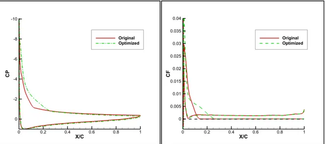
Figure 4.5 Pressure distributions and skin friction coefficient comparisons at 34 m/s and 10 deg angle of attack ...89
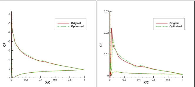
Figure 4.6 Pressure distributions and skin friction coefficient comparisons at 34 m/s and 15 deg angle of attack ...89
Figure 4.7 Pressure distributions and skin friction coefficient comparisons at 34 m/s and 19 deg angle of attack ...90
Figure 4.8 Original and optimized airfoils lift and drag variations comparison at Mach 0.10...91
Figure 4.9 Original and optimized airfoils lift/drag ratio comparison at Mach 0.10...92
Figure 4.10 Pressure distributions and skin friction coefficient comparisons at 51 m/s and 10 deg angle of attack ...93
Figure 4.11 Pressure distributions and skin friction coefficient comparisons at 51 m/s and 15 deg angle of attack ...94
Figure 4.12 Pressure distributions and skin friction coefficient comparisons at 51 m/s and 19 deg angle of attack ...94
Figure 4.13 Original and optimized airfoils lift and drag variations comparison at Mach 0.15...95
Figure 4.14 Original and optimized airfoils lift and drag variations comparison
at Mach 0.20...95
Figure 4.15 Chord-wise positions of the boundary layer separation points for Re = 1.41 million (left), Re = 2.17 million (center) and Re = 2.82 million (right) ...96
Figure 4.16 Comparison between the original airfoil and three optimized airfoils ...98
Figure 5.1 The morphing skin for the airfoil ...107
Figure 5.2 The NURBS control points for the original airfoil ...109
Figure 5.3 Direction of movement and imposed limits for a control point ...109
Figure 5.4 General outline of the ABC algorithm ...112
Figure 5.5 Setup for airfoil optimization problem using modeFrontier ...117
Figure 5.6 Choice of parameters for MOGA-II algorithm ...117
Figure 5.7 Original and optimized airfoils drag polar comparison for Mach = 0.15 ...120
Figure 5.8 Drag coefficient reduction over the lift coefficient range for Mach = 0.15 ...120
Figure 5.9 Original and optimized airfoils lift over drag ratio comparison for Mach = 0.15 ...121
Figure 5.10 Pressure distributions and skin friction coefficient comparisons at 51 m/s and 2 deg angle of attack ...123
Figure 5.11 Pressure distributions and skin friction coefficient comparisons at 51 m/s and 10 deg angle of attack ...123
Figure 5.12 Drag coefficient reduction over the lift coefficient range for Mach = 0.10 ...124
Figure 5.13 Drag coefficient reduction over the lift coefficient range for Mach = 0.20 ...124
Figure 5.14 Comparison of the upper surface transition location with the angle of attack for Mach 0.15 ...126
Figure 5.15 Original and optimized airfoils drag polar comparison for Mach = 0.15 ...126
Figure 5.16 Pressure distributions comparisons at 51 m/s and -1 deg angle of
attack (left) and 3 deg angle of attack (right) ...127
Figure 5.17 Comparison of the upper surface transition location with the angle of attack for Mach 0.10 ...128
Figure 5.18 Comparison of the upper surface transition location with the angle of attack for Mach 0.20 ...128
Figure 5.19 Comparison between the original airfoil and three optimized airfoils ....132
Figure 6.1 Chordwise section through the morphing wing (left) and topside view of the morphing skin (right) ...139
Figure 6.2 Control points for one spanwise section (left) and the movement constraints for one selected point (right) ...141
Figure 6.3 Horseshoe vortices distribution over the wing surface ...142
Figure 6.4 Geometry details for a typical horseshoe vector ...143
Figure 6.5 Details of the morphing wing optimization procedure ...147
Figure 6.6 The modification of the upper surface morphing skin shape control using three spanwise actuation lines ...152
Figure 6.7 Spanwise variation of lift, induced drag and profile drag coefficients at a -2 deg angle of attack ...154
Figure 6.8 Pressure coefficient distributions for y=1.0 (upper) and y=1.8 (lower) sections at a -2 deg angle of attack ...155
Figure 6.9 Spanwise variation of lift, induced drag and profile drag coefficients at a 1 deg angle of attack ...156
Figure 6.10 Pressure coefficient distributions for y=1.0 (upper) and y=1.8 (lower) sections at a 1 deg angle of attack ...157
Figure 6.11 Spanwise variation of lift, induced drag and profile drag coefficients at a 4 deg angle of attack ...158
Figure 6.12 Pressure coefficient distributions for y=1.0 (upper) and y=1.8 (lower) sections at a 4 deg angle of attack ...159
Figure 6.13 Spanwise variation of lift, induced drag and profile drag coefficients at a 8 deg angle of attack ...160
Figure 6.14 Pressure coefficient distributions for y=1.0 (upper) and y=1.8 (lower) sections at a 8 deg angle of attack ...161 Figure 6.15 Cut of the UAS-S4 H-Type structured mesh ...164 Figure 6.16 Typical residual convergence curves ...164 Figure 6.17 Plot of turbulent kinetic energy on the upper surface on the original
wing (left) and the Case 5 morphed wing (right) at a 1 deg
angle of attack ...166 Figure 6.18 Plot of turbulent kinetic energy on the upper surface on the original
wing (left) and the Case 5 morphed wing (right) at a 4 deg
angle of attack ...166 Figure 6.19 Pressure coefficient distributions for y=1.0 sections at a 1 deg
angle of attack ...167 Figure 6.20 Pressure coefficient distributions for y=1.8 sections at a 1 deg
angle of attack ...168 Figure 6.21 Pressure coefficient distributions for y=1.0 sections at a 4 deg
angle of attack ...169 Figure 6.22 Pressure coefficient distributions for y=1.8 sections at a 4 deg
angle of attack ...170 Figure 7.1 Vortex rings over the mean camber surface of a typical wing ...179 Figure 7.2 Details of a six-edged vortex ring placed over a wing panel ...179 Figure 7.3 Span-wise strips and surface panels division of example
half wing geometry ...183 Figure 7.4 Neighbouring rings for a general, arbitrary vortex ring of the
wing model...186 Figure 7.5 Convergence of the aerodynamic coefficients with
grid refinement level ...194 Figure 7.6 Residual convergence curves with grid refinement level ...195 Figure 7.7 Pressure coefficient variation for a flat plate, compared to exact linear
potential theory ...196 Figure 7.8 Numerical versus experimental lift coefficient variation with the
Figure 7.9 Numerical versus experimental drag coefficient variation with the lift coefficient for the NACA TN 1270 wing ...199 Figure 7.10 Numerical versus experimental pitching moment coefficient variation
with the lift coefficient for the NACA TN 1270 wing ...200 Figure 7.11 Numerical versus experimental lift coefficient variation with the
angle of attack for the NACA TN 1208 wing ...202 Figure 7.12 Numerical versus experimental pitching moment coefficient variation
with the lift coefficient for the NACA TN 1208 wing ...202 Figure 7.13 Comparison of span-wise loading for the NACA TN 1208 wing at
4.7 degrees angle of attack ...203 Figure 7.14 Numerical versus experimental lift coefficient variation with the
angle of attack for the NACA RM L50F16 wing ...205 Figure 7.15 Numerical versus experimental drag coefficient variation with the lift
coefficient for the NACA RM L50F16 wing ...205 Figure 7.16 Numerical versus experimental pitching moment coefficient variation
with the lift coefficient for the NACA RM L50F16 wing ...206 Figure 7.17 Comparison between the original and the redesigned wing
and airfoil shapes ...208 Figure 7.18 Comparison between the lift and drag coefficients for the original
and redesigned wings ...211 Figure 7.19 Comparison between the lift and drag coefficients for the original
and morphed wings ...216 Figure 8.1 The position of the morphing skin on the aircraft wing ...225 Figure 8.2 The structural elements of the CRIAQ MDO 505 morphing wing
concept (the morphing skin is not shown in the figure) ...225 Figure 8.3 CRIAQ MDO 505 morphing wing concept ...227 Figure 8.4 Overview of the morphing wing control system ...229 Figure 8.5 Marker positions for the un-deformed upper skin ...234 Figure 8.6 Interpolated point grid constructed from the scanned marker positions
Figure 8.7 Chord-wise cross-section view of the mesh ...238 Figure 8.8 Span-wise cross-section view of the mesh ...238 Figure 8.9 MDO 505 wing model setup in the wind tunnel test section ...240 Figure 8.10 IR visualisation of the laminar-to-turbulent transition region on the
upper surface for both un-morphed (left) and morphed (right)
skin shapes ...241 Figure 8.11 Transition for Case 39 un-morphed using the
turbulence intermittency ...243 Figure 8.12 Comparison between numerical and IR experimental transition
detection for the station located at 40% of the span, for the cases
C39 – C45 un-morphed and morphed wings ...244 Figure 8.13 Comparison between numerical and IR experimental transition
detection for the station located at 40% of the span, for the cases
C68 – C73 un-morphed and morphed wings ...245 Figure 8.14 Comparison between numerical and IR experimental transition
detection for the station located at 40% of the span, for the cases
C74 – C82 un-morphed and morphed wings ...245 Figure 8.15 Comparison between experimental and numerical transition location
on the wing upper surface for case C40, for both un-morphed (left)
and morphed (right) geometries ...248 Figure 8.16 Comparison between experimental and numerical transition location
on the wing upper surface for case C72, for both un-morphed (left)
and morphed (right) geometries ...249 Figure 8.17 Comparison between experimental and numerical transition location
on the wing upper surface for case C77, for both un-morphed (left)
and morphed (right) geometries ...250 Figure 8.18 Comparison of experimental versus numerical pressure coefficient
distribution for case C40 un-morphed (left) and morphed (right) ...252 Figure 8.19 Comparison of experimental versus numerical pressure coefficient
distribution for case C68 un-morphed (left) and morphed (right) ...252 Figure 8.20 Comparison of experimental versus numerical pressure coefficient
Figure 8.21 Comparison of experimental versus numerical pressure coefficient
LIST OF ABREVIATIONS
ABC Artificial Bee Colony optimization algorithm
ALM Augmented Lagrangian Method
ATAG Air Transport Action Group
BFGS Broyden-Fletcher-Goldfarb-Shanno optimization algorithm CFD Computational Fluid Dynamics
CIRA Italian Aerospace Research Center (Centro Italiano Ricerche Aerospaziali) CNRC Canada National Research Council
DLM Doublet Lattice Method
DLR German Aerospace Research Center (Deutsches Zentrum fur Luft und Raumfahrt)
EADS European Aeronautic Defence and Space Company ETS École de Technologie Supérieure
GA Genetic Algorithm
IAR-CNRC Institute for Aerospace Research – Canadian National Research Center ICAO International Civil Aviation Organization
LARCASE Laboratory of Applied Research in Active Control, Avionics and Aeroservoelasticity
LLM Lifting Line Method
MAC Mean Aerodynamic Chord
MDO Multi-Disciplinary Optimization NACA National Advisory Committee for Aeronautics NASA National Aeronautics and Space Administration NURBS Non-uniform Rational B-Splines
SMA Shape Memory Alloy SST Shear Stress Transport
UAS Unmanned Aerial System
UAV Unmanned Aerial Vehicle
LIST OF SYMBOLS AND UNITS OF MEASUREMENTS
Aerodynamic influence coefficients for the VLM Surface of a wing panel/strip
Wing span
Elements of the linear system right hand side for the VLM
Wing half-span
Approximate Hessian matrix Chord of a wing strip
Unit vector in the direction of the local chord for a wing strip
Airfoil chord
Drag coefficient of a wing strip airfoil Lift coefficient of a wing strip airfoil Wing drag coefficient
Wing profile drag coefficient Wing induced drag coefficient Skin friction coefficient Wing lift coefficient
Derivative of lift coefficient with the angle of attack Wing pitching moment coefficient
Derivative of pitching moment coefficient with the angle of attack ∆ Pressure coefficient variation between wing upper and lower surfaces
( ) Point on a NURBS curve
Wing drag
Objective function to be minimized
Force vector acting on the bound segment of a horseshoe vortex Aerodynamic force generated by the wing
Aerodynamic force acting on a panel/strip of the wing surface
Equality constraints ℎ Static enthalpy ℎ Inequality constraints Total enthalpy ̅ Unit tensor Jacobian matrix
Turbulent kinetic energy
Number of NURBS control points Length of the flexible skin
Vector along the bound segment of a horseshoe vortex
Wing lift
Mach number
Quarter chord moment of a wing strip
Aerodynamic moment about the root chord quarter chord point generated by the wing
Order of the NURBS curve
Number of horseshoe/ring vortices and panels on the wing surface Chordwise number of panel on the wing surface
Spanwise number of panel on the wing surface , NURBS curve basis functions
Static pressure
Reference pressure
BFGS method search direction Turbulent Prandtl number Control point of a NURBS curve Freestream dynamic pressure Vector along a vortex segment
Vector from the beginning of a vortex segment to an arbitrary point in space Vector from the end of a vortex segment to an arbitrary point in space
Position vector of wing strip quarter chord and panel collocation point with reference to root chord quarter chord point
Nonlinear system of equations
Reynolds number
Critical Reynolds number
Momentum thickness transition Reynolds number
Wing area
NURBS curve knot
Air temperature
Component of the fluid velocity field
Unit vector in the direction of the freestream flow
Velocity induced by horseshoe/ring vortex , considered to be of unit intensity, at the control point of horseshoe/ring vortex
Modulus of surface transpiration velocity Velocity vector
Freestream velocity vector
Local velocity at the bound segment of a horseshoe vortex and at the collocation point of a ring vortex
Surface transpiration velocity vector NURBS curve weight
Optimization problem solution
Chordwise coordinate
Upper surface transition point location
Solution vector for the nonlinear system of equations ∆ Span of a wing strip
Difference between two successive estimations of the gradient
Spanwise coordinate
Geometric angle of attack of the wing Local angle of attack for a wing strip BFGS method advancement step Penalty coefficient control parameter Intermittency
Geometric vector along the edge of a vortex ring
Vortex intensity
∆ Vortex intensity correction
Displacement of a NURBS control point Kronecker delta function
Upper limit for NURBS control point movement Lower limit for NURBS control point movement
Thermal conductivity
Lagrangian multipliers
Air dynamic viscosity
Effective viscosity
Turbulent viscosity
Air density
̅ Fluid stress tensor
Perturbation potential
Modified objective function
Freestream potential
Specific dissipation rate
INTRODUCTION
The air transportation industry is one of the key areas that contribute to the economic development around the world. Although only 0.5 % of the total volume of international trading is done by air, this small volume accounts for almost 35% of the total trade value (ATAG, 2014), aircrafts being used especially for high value, time sensitive merchandise. Since the beginning of civil aviation, there has also been a steady increase in the number of people using airplanes as a fast and safe transportation method, airlines carrying almost 3 billion passengers in 2014 alone. This high level of development that has been achieved by the industry has also transformed it into a major source of pollution. It is estimated that in 2014, over 2% of the worldwide carbon dioxide emissions were caused by the commercial airline companies (ATAG, 2014).
The high growth rate of aviation traffic experienced up to present day will accelerate over the next decades. The International Civil Aviation Organization (ICAO) estimates that the number of flights will triple by the year 2050 (ICAO, 2010). This high growth rate, together with growing global concern for the preservation of the environment and the reduction of greenhouse gas emissions obliges the aerospace industry to search for solutions to improve the efficiency of aircraft. According to the 2014 United Nation Climate Summit, in order to promote sustainable development and to minimize the impact on future climate changes, the aviation industry should improve its fuel efficiency by 1.5% per year, and by 2050 achieve net carbon dioxide emission that will be half of what they were in 2005, despite the predicted increase in the number of flights (ATAG, 2014). Figure 0.1 presents the estimated net emission of carbon dioxide of the air transport industry up to 2050, depending on the number of solutions adopted in order to provide the required efficiency increase.
Figure 0.1 Estimation of carbon dioxide emission for the aviation sector, in function of the number of actions taken to increase efficiency.
Taken from ATAG (2014)
One possibility of achieving this desired efficiency is the new-generation technology of wing morphing, the active and controlled modification of one or several wing characteristics during flight. Today’s aircraft are designed during a multi-point optimization process, meaning that they perform well over a range of different flight conditions, but the performance is sub-optimal for each flight condition. In theory, a morphing wing could allow the aircraft to fly at optimal lift to drag ratios for each condition encountered during a flight, by changing its wing’s characteristics and controlling them according to the flow conditions. The approach represents, in essence, a single-point optimization of the wing geometry, performed for each different flight condition, thus eliminating the compromises associated with today’s multi-point optimization approach.
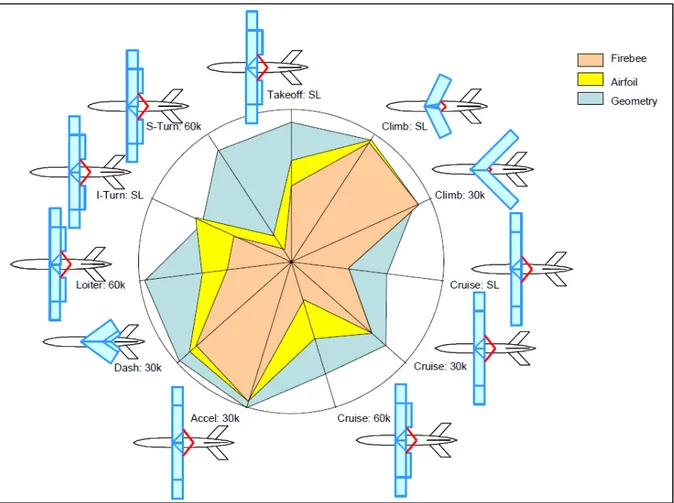
In Figure 0.2, a performance plot is presented for the BMQ-34 Firebee unmanned target drone, for different flight conditions (take-off, climbing, cruise, loitering and manoeuvring), at various altitudes (sea level, 30,000 feet and 60,000 feet). The performance plot, created through the research of Joshi et al. (2004), shows the performance of the drone for the chosen conditions, as well as the theoretical performance that could be achieved by equipping the drone with a morphing wing capable of airfoil changes and a morphing wing capable of
geometry changes. It can be seen that the use of the morphing wing can substantially increase the flight performance of the unmanned drone, for nearly all of the analysed cases.
Figure 0.2 Performance increase achieved for various flight conditions by using a morphing wing technology.
Taken from Joshi et al. (2004)
Researchers have proposed different technological solutions for obtaining the desired wing adaptability, and some concepts achieved important theoretical performance improvements compared to the baseline design. However, the technology being only in its first phases of development, its technological readiness level is still very low, and only a few concepts have been sufficiently progressed to reach wind tunnel testing, and even fewer have actually been flight tested (Barbarino et al., 2011).
Morphing architectures are a promising solution for the development of the next generation of green aircraft, and many large industry companies are investigating the benefits of this technological approach. However, there is still a lack of sufficient applied research projects that clearly present the possible advantages, due to the high costs involved in developing functional wind tunnel or flight-worthy morphing models. Under these conditions, Unmanned Aerial Vehicles (UAVs) have become the system of choice for the investigation of morphing aircraft solutions, due to much lower costs needed for the development, implementation, and finally flight testing of the morphing system.
0.1 Problem Statement
With the increasing role of Unmanned Aerial Vehicles in surveillance and combat operations, an increase in their operational range, agility and versatility is necessary. A morphing wing system could prove a viable technological solution that would allow the UAV to achieve the desired efficiency. The reasons for developing shape morphing UAVs can be summarized with the following three objectives in mind (Barbarino, 2009):
• adaptability, by making the aircraft more versatile and thus suitable for a wider range of flight conditions;
• multi-objective, by trying to accommodate one aircraft to diverse, even contradictory mission scenarios, and performing all of them as efficiently as possible;
• efficiency, leading to improved, intelligent structures, capable of better efficiency in terms of energy consumption.
Civil aviation could also greatly benefit from the performance gains that a morphing wing system could provide. The ability to increase the extent of laminar flow over the wing surface for all flight conditions that occur during a typical flight, as well as the reduction of the upper surface shock wave intensity during cruise flight could lead to significant reductions in drag, and thus in fuel consumption. The morphing wing approach could eliminate some of the compromises associated with today’s aircraft design procedures, allowing the industry to increase the efficiency of their products.
The research presented in this thesis was performed as part of two projects: the Hydra Technologies S4 Éhecatl Unmanned Aerial System (UAS) morphing wing, and the CRIAQ MDO 505 morphing wing, designed based on the wing tip of a typical passenger aircraft.
0.1.1 Hydra Technologies S4 Éhecatl morphing wing
The UAS-S4 Éhecatl was obtained by Prof. Ruxandra Botez from Canada Foundation for Innovation (CFI) and Ministère du Développement Économique, Innovation et Exportation (MDEIE), and was designed and build in Mexico by Hydra Technologies. It was created as an unmanned aerial surveillance system, directed towards providing security and surveillance capabilities for the Armed Forces, as well as civilian protection in hazardous situations. The existence of this aircraft at ÉTS will make possible the design, construction and implementation of the morphing wing system, and thus will provide experimental flight test data in addition to the numerical research presented in this thesis. General information about the characteristics and flight performance of the UAS-S4 Éhecatl is presented in Table 0.1, while the aircraft is shown in Figure 0.3.
Table 0.1 General information about the UAS-S4 Éhecatl
Characteristic Value
Empty Weight 50 kg
Maximum Take-off Weight 80 kg
Wingspan 4.2 m
Mean Aerodynamic Chord 0.57 m
Wing Area 2.3 m2
Total Length 2.5 m
Operational Ceiling 15,000 ft
Maximum Airspeed 135 knots
Loitering Airspeed 35 knots
Figure 0.3 Hydra Technologies UAS-S4 Éhecatl
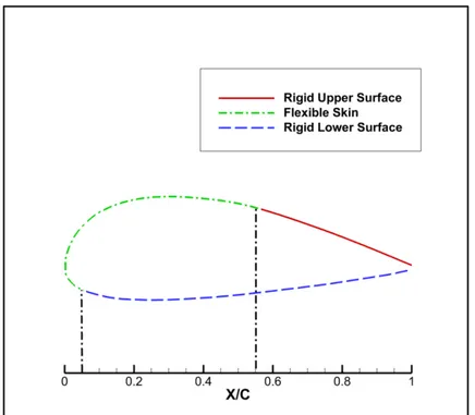
In order to provide the desired increase in aerodynamic efficiency, the conventional rigid wing of the UAS-S4 is replaced with a morphing wing equipped with a flexible upper surface and leading edge, capable of actively changing the wing's airfoil, depending on the flight condition. In order to implement the wing morphing technique on the UAS, only a limited portion of wing surface can be allowed to change, and the shape modifications introduced must be small enough in order for the concept to remain feasible from a structural point of view.
0.1.2 CRIAQ MDO 505 morphing wing
The CRIAQ MDO 505 Morphing Wing project is an international collaboration between Canadian and Italian industries (Bombardier Aerospace, Thales Canada and Alenia Aeronautica), universities (École de Téchnologie Supérieure, École Polytechnique and University of Naples) and research centers (Canada National Research Council and Italian Aerospace Research Center). The research in this project is focused on demonstrating the structural, aerodynamic and control abilities of a morphing technology demonstrator model,
designed after an aircraft wing tip, equipped with an adaptive upper surface and both rigid and adaptive ailerons during low speed wind tunnel tests.
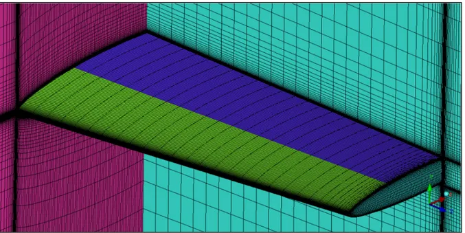
The full-scale model is an optimized, flexible structure with a 1.5 m span and a 1.5 m root chord and has a taper ratio of 0.72 and a leading edge sweep angle of 8 deg. The wing box and internal structure are manufactured from aluminum, with the composite adaptive upper surface extending from 20% to 65% of the wing chord. The adaptive upper surface was specifically designed and optimised for this project from carbon composite materials. The actuators were also specifically designed and manufactured to the project requirements. Four electric actuators are installed on two actuation lines, fixed to the center ribs and to the composite skin. Each actuator is capable of independent action. On each line the actuators are situated at 32% and 48% of the chord. The aileron (conventional and adaptive) articulation is situated at 72% of the chord. Figure 0.4 presents the concept of the morphing wing and a cross-section view of the model.
0.2 Research Objectives
The global objective of the research is to provide an accurate calculation of the performance improvements that could be obtained for both the UAS-S4 and MDO 505 wings by using the flexible skin morphing wing technology, and to determine the wing surface shape changes required to obtain the desired improvements. For the UAS-S4, the analysis is performed for a number of different airspeeds and for a wide range of angles of attack, in order to cover a significant part of the aircraft’s flight envelope. For the MDO 505 wing, a number of wind tunnel test cases were established in agreement with all project partners and the analysis is performed for these cases.
To ensure a good progress of the research and to successfully achieve the proposed global objective, the following sub-objectives were established:
1) Conception of geometry parameterization techniques and new optimization algorithms
• The implementation of a Non-Uniform Rational B-Splines (NURBS) methodology for the parameterization of the UAS airfoil and for generating smooth and continuous shapes for the morphed airfoil;
• Further development of the NURBS parameterization methodology in order to allow only a local airfoil shape modification, between some desired chordwise limits;
• The implementation of different constrained global optimization algorithms, such as Genetic Algorithm and Artificial Bee Colony algorithm;
• Further development of the constrained global optimization algorithm in order to accelerate their convergence properties, by performing a hybridisation with a modified version of the gradient-based Broyden-Fletcher-Goldfarb-Shanno optimization algorithm.
2) Application of these methodologies and algorithms for the performance improvement of the UAS-S4 morphing airfoil
• Performing two-dimensional optimizations of the UAS-S4 airfoil with the objective of reducing the airfoil drag coefficient and increasing the region of laminar flow, for a wide range of angles of attack below stall;
• Performing two-dimensional optimizations of the UAS-S4 airfoil with the objective of increasing the maximum lift coefficient and delaying boundary layer separation for angles of attack at stall and immediately after stall.
3) Conception of new aerodynamic methods and solvers
• The development and implementation of a non-linear lifting line method capable of providing an accurate estimation of the UAS-S4 wing aerodynamic coefficients, including a calculation of the viscous drag component;
• The development and implementation of a quasi-three-dimensional non-linear vortex lattice method, capable of providing accurate viscous calculations of the aerodynamic coefficients for wing of various geometric shapes.
4) Application of the new solvers and algorithms for the performance improvement of the UAS-S4 morphing wing
• Further development of the NURBS parameterization methodology in order to allow the reconstruction of the entire three-dimensional morphed wing surface, by performing cubic splines interpolations in the span direction;
• Performing three-dimensional optimizations of the UAS-S4 wing with the objective of increasing the lift-to-drag ratio for a wide range of angles of attack below stall, and analysing the impact of different configurations of the morphing wing approach on the performance gains;
• Performing three-dimensional viscous redesign and optimization of the UAS-S4 morphing wing, with the objective of increasing the lift-to-drag ration, but also an optimization of the low aspect ratio MDO 505 morphing wing, with the goal of reducing the profile drag coefficient.
5) Application of high-fidelity solvers for the performance improvement of the MDO 505 morphing wing and results validation with experimental data
• The adaptation of the three-dimensional surface reconstruction algorithms for generating the MDO 505 morphing skin shapes in function of the actuator displacements;
• The development of an automated procedure for the generation of high-quality structured meshes around the MDO 505 wing, capable of working with the entire range of flexible skin actuators’ displacements and aileron deflection angles;
• Performing three-dimensional analysis of the MDO 505 morphing wing with the objective of accurately determining the laminar-to-turbulent transition region and increasing the region of laminar flow;
• Validation of the numerical results using experimental data obtained in the CNRC subsonic wind tunnel during the MDO 505 project testing phase.
0.3 Research Methodology and Models
In order to perform the numerical analysis of a morphing wing system, several different algorithms and codes, both originally developed and commercially available, were coupled and used:
• the NURBS and cubic splines interpolations for generating the morphed airfoil and wing geometries;
• the Genetic and the hybrid Artificial Bee Colony - Broyden-Fletcher-Goldfarb-Shanno algorithms for determining the optimum wing shapes in function of the flight conditions; • the XFOIL solver for performing the two-dimensional aerodynamic calculations;
• the novel non-linear lifting line method and the original non-linear vortex lattice method for performing the fast three-dimensional aerodynamic calculations and optimizations; • the ICEM-CFD code for generating the high-quality meshes around the morphing wings; • the FLUENT solver for performing high-fidelity three-dimensional aerodynamic
Each one of these models will be briefly presented and explained. All the algorithms developed during the research were programmed using FORTRAN and C, saved and compiled as self-contained 32-bit applications, without requiring any additional libraries. They can be run on any computer using the Windows XP, Vista, Seven, Eight or Ten operating systems, both 32-bit and 64-bit versions. The desired configuration and setup is performed using input files of simple formatting (TXT or DAT files, modifiable by any text editor), and the output is presented in the same way, and can be further post-processed.
0.3.1 Non-Uniform Rational B-Splines
From a numerical point of view, the airfoil was parameterized using Non-Uniform Rational B-Splines (NURBS) (Piegl and Tiller, 1997). The NURBS are a generalization of B-Splines and Bézier curves, offering high flexibility and precision in representing and manipulating analytical curves. From a mathematical point of view, its order, a polygon of weighted control points, and a knot vector define a NURBS curve:
( )
, 1 , 1 k i n i i k i j n j j N w u N w = = =
C P (0.1)In the above Equation (0.1), is the curve parameter, ranging from 0 (the start of the curve) to 1 (the end of the curve), is the number of control points, , is the basis function, of order , is the weight associated with the control point, and = , ] is the control point. The basis functions are determined using the De Boor recursive formula (De Boor, 1978): 1 ,1 1 , , 1 1, 1 1 1 1 , if 0 , otherwise i i i i i n i n i n i n i n i i n i t u t N u t t u N N N t t t t + + + − + − + + + + ≤ ≤ = − − = + − − (0.2)
where is again the curve parameter, is the order of the basis function, while represents the knot of the curve knot vector.
When an airfoil curve is given as input, the positions of the control points and the distribution of knots along the curve length are determined through an iterative least-squares curve fitting process (Piegl and Tiller, 1997). As an example, the NACA 4409 airfoil is presented in Figure 0.5, together with the NURBS control polygon associated with it, as resulted from the curve fitting procedure. The vertical coordinate was significantly expanded in order to provide better visualization.
Figure 0.5 Example airfoil and the associated NURBS control points
For the parameterization of the airfoil curves, a 3rd degree NURBS curve has been used, which grants smoothness up to the second derivative. The number of control points associated with a given airfoil depends on the tolerance imposed during the curve fitting process. In general, a number of 12 to 15 NURBS control points is enough to accurately construct an approximation of an airfoil. If more NURBS control points are desired, to
provide better control of the local shape during the airfoil optimization process, the extra control points can be added on the initial control polygon, between the initial points, without affecting the quality of the obtained initial fitting.
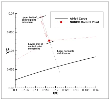
To allow the realization of a local modification of the airfoil shape, between some desired points along the airfoil curve length, extra knots were inserted in the NURBS knot vector, in order to clearly mark the limits of the region that changes during the optimization. The control points that correspond to this marked region were then redistributed using a second least-squares curve fitting process, thus providing the desired accuracy, number and distribution of control points needed to control the airfoil local shape change. During the numerical optimization procedure, the morphing of the airfoil curve shape was achieved by changing the coordinates of the NURBS control points.
0.3.2 Cubic splines
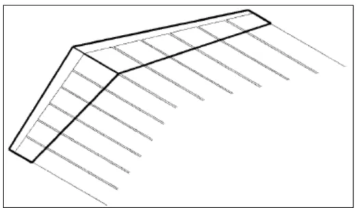
The NURBS method is used to parameterize and morph the shape of the airfoil, for the two-dimensional optimization process, and the wing morphing control airfoil sections, placed at several positions along the span, for the three-dimensional optimization process. These airfoil sections correspond to the span-wise positions of the mechanical actuation system lines used to generate the wing surface shape change, and thus only a small number (between 2 and 5) of such wing sections are present on each semi-span. In order to accurately reconstruct the morphed wing surface, this small number of the actuation system sections is not sufficient and more wing airfoil sections must be generated. To achieve this, cubic splines are used to perform interpolations between any two consecutive actuation system sections, and thus generate the required number of wing sections.
Figure 0.6 presents an example of wing geometry created with several airfoil sections along the span direction. Out of these sections, 4 were parameterized using NURBS and then modified (thus simulating the actuation of the wing morphing system), while the other sections were reconstructed with cubic splines interpolations, based on the four main control
sections. Using this procedure, there are enough wing sections along the span to accurately generate the complete morphing wing geometry.
Figure 0.6 Example wing geometry created with several airfoil sections along the span direction
Cubic splines were chosen for the interpolation because of their similarity with the theoretical behaviour of a beam that is bending under uniform loading, and because of their ability to provide very good tangency conditions between two consecutive spline curves, by ensuring smoothness up to the second derivative (Berbente, 1998).
0.3.3 The Genetic Algorithm optimizer
Genetic algorithms are numerical optimization algorithms inspired by natural selection and genetics of living organisms. The algorithms are initialized with a population of guessed individuals, and use three operators namely selection, crossover and mutation to direct the population towards its convergence to the global optimum, over a series of generations (Coley, 1999).
In order to evaluate all individuals in the population, an objective function, called the fitness function, must be defined. This fitness function is calculated for all individuals of a given generation. The higher the values of the fitness function, the higher are the chances of the individual to be selected for the creation of the next generation.
The general outline of the method and all the steps of the genetic algorithm are presented in Figure 0.7. The process of evaluation of the fitness function, selection of the best individuals to become parents, crossover and mutation of the new individuals continues in an iterative way, until the maximum number of generations is reached. Tournament selection, simulated binary crossover (Herrera, 1998) and polynomial mutation (Herrera, 1998) were used. The termination criterion used was the achievement of the maximum number of generations.
0.3.4 Artificial Bee Colony optimizer
The ABC algorithm is an optimization algorithm based on the intelligent behaviour of a honeybee swarm. Karaboga and Basturk conceived the original algorithm in 2007 (Karaboga and Basturk, 2007), that was applicable only to the unconstrained optimization of linear and nonlinear problems. Other authors have proposed methods for enhancing the algorithm’s capabilities, such as the handling of constrained optimization problems (Karaboga and Basturk, 2007) or the significant improvement of its convergence properties (Zhu and Kwong, 2010). Because of the fact that the ABC algorithm simultaneously performs a global search throughout the entire definition domain of the objective function and a local search around the more promising solutions already found, it can efficiently avoid converging towards a local minimum point of the objective function, and thus is able to approximate the global optimum point.
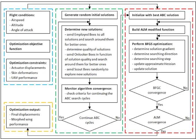
It was discovered that for some problems, after the region of the global optimum was found, the ABC algorithm’s rate of convergence significantly decreased. To improve convergence, the ABC method’s search routine was substituted by the Broyden-Fletcher-Goldfarb-Shanno (BFGS) algorithm (Bonnans et al., 2006), a type of quasi-Newton iterative method used for nonlinear optimization problems. Since the BFGS method can only be applied to unconstrained optimization, it was coupled with the Augmented Lagrangian Method (ALM) (Powell, 1967) in order to introduce the desired optimization constraints. The use of the ALM-BFGS approach allows obtaining a significantly faster determination of the global optimum position, thus accelerating the convergence rate of the final steps of the optimization procedure. The details of the hybrid ABC and BFGS algorithms, the coupling between them, as well as the general configuration of the morphing wing optimization procedure are presented in Figure 0.8.
Figure 0.8 Artificial Bee Colony algorithm coupled with the ALM-BFGS algorithm
0.3.5 Two-dimensional flow solver
The code that was used for the calculation of the two-dimensional aerodynamic characteristics of the airfoil is XFOIL, version 6.96, developed by Drela and Youngren (2001). The XFOIL code was chosen because it has proven its precision and effectiveness over time, and because it reaches a converged solution very fast (the order of a few seconds). The inviscid calculations in XFOIL are performed using a linear vorticity stream function panel method (Drela, 1989). A Karman-Tsien compressibility correction is included, allowing good predictions for subsonic, incompressible and compressible flows. For the viscous calculations, XFOIL uses a two-equation lagged dissipation integral boundary layer formulation (Drela, 1989), and incorporates the transition criterion (Drela, 2003). The flow in the boundary layer and in the wake interacts with the inviscid potential flow by use of
the surface transpiration model. The nonlinear system of equations formed by the inviscid flow equations and the boundary layer model equations is solved using Newton’s method.
The transition criterion models the growth of Tollmien-Schlichting (TS) waves in the laminar boundary layer, and it permits tracking the true critical frequency by using the amplification rates of the TS waves that are obtained from solutions of the Orr-Sommerfeld equation. Laminar-to-turbulent transition onset depends on the turbulence intensity level of the incoming airflow. In the method, this dependence is accounted for by adjusting the critical amplification factor to values that are representative for the analysed flow conditions. For the research presented here, values of 9 and 10 were used, corresponding to calm atmospheric conditions. Because the morphing skin concept is effective at delaying laminar-to-turbulent transition, its performance is directly influenced by the turbulence intensity level of the airflow. A morphed geometry that outperforms the baseline design at a given flight condition (expressed in terms of airspeed, angle of attack, Reynolds number and turbulence intensity) may decrease (or increase) its efficiency for other critical amplification factor values. A detailed sensitivity analysis of the performance improvements obtained with the morphing skin concept, as function of various turbulence intensity levels must be performed. The study will provide a better understanding of the morphing skin behaviour in airflow conditions other than the calm, standard atmosphere model.
0.3.6 Nonlinear lifting line method
Prandtl's classical lifting line theory, first published in 1918, represented the first analytical model capable of accurately predicting the lift and induced drag of a finite span lifting surface. The aerodynamic characteristics predicted by the theory were repeatedly proven to be in close agreement with experimental results, for straight wings with moderate to high aspect ratio. The theory was based on the hypothesis that a finite span wing could be replaced by a continuous distribution of vorticity bound to the wing surface, and a continuous distribution of shed vorticity that trails behind the wing, in straight lines in the direction of the free stream velocity. The intensity of these trailing vortices is proportional to rate of
change of the lift distribution along the wing span direction. The trailing vortices induce a velocity, known as downwash, normal to the direction of the free stream velocity, at every point along the span. Because of the downwash, the effective angle of attack at each section in the spanwise direction is different from the geometric angle of attack of the wing, the difference being called the induced angle of attack. Using the effective angle of attack, the downwash produced by the trailing vortices and the two-dimensional Kutta-Joukowski vortex lifting law, Prandtl developed an integral equation that allowed the calculation of the continuous bound vorticity intensity, and thus the calculation of the wing's lift and induced drag.
The nonlinear method uses a general horseshoe vortex distribution and a fully three-dimensional vortex lifting law (Sugar Gabor, 2013). Because of these characteristics, the method has a wider applicability range compared to the original theory, as it can analyse multiple lifting surfaces placed in the same flow field and the wings that have arbitrary camber, sweep angle and dihedral angle. Also, the method is not based on the assumption of a linear relationship between the lift coefficient and the local angle of attack, thus it can be applied for high geometric angles of attack, to take into consideration the effects of stall. The constraint of medium to high aspect ratio lifting surface that applies to Prandtl's original theory also applies to the nonlinear method.
Using the three-dimensional vortex lifting law, the force acting on any of the horseshoe vortices placed on the wing surface can be written as follows:
i = Γ ×ρ i i i
dF V dl (0.3)
In the above equation, is the air density, is the unknown intensity of the horseshoe vortex, is the local airflow velocity and is a spatial vector along the bound segment of the horseshoe vortex, aligned in the direction of the local circulation. The local airfoil velocity is equal to:
1 N i j ij j ∞ = = +
Γ V V v (0.4)where is the free stream velocity, while represents the velocity induced by the horseshoe vortex , considered to be of strength equal to unity, at the control point of horseshoe vortex .
From the wing strip theory, the magnitude of the aerodynamic force acting on a section of the wing located at a given span location on the wing can be written as:
2 1
2 i li
i = ρV A C∞
F (0.5)
The lift coefficient is the coefficient of the local airfoil situated at the wing span section corresponding to control point and depends on the local effective angle of attack, while is the area of the considered strip.
If the strip lift coefficient can be determined using other means, such as experimentally determined lift curves or using a two-dimensional airfoil calculation solver, then, by replacing the local velocity given by Equation (0.4) into Equation (0.3), and then equating the modulus of the three-dimensional vortex lifting force presented in Equation (0.3) with the expression given in Equation (0.5), the following nonlinear equation is obtained:
2 1 1 2 i N i j ij i i l j V AC ρ ∞ ρ ∞ = Γ + Γ × = V
v dl (0.6)Writing Equation (0.6) for all the horseshoe vortices on the wing surface, a nonlinear system is obtained that can be solved using Newton’s method in order to obtain the unknown vortex intensities. The method presented can be used to calculate the profile drag coefficient of the