Montréal
Série Scientifique
Scientific Series
2001s-25Simulation-Based Finite-Sample
Tests for Heteroskedasticity
and ARCH Effects
Jean-Marie Dufour, Lynda Khalaf,
Jean-Thomas Bernard, Ian Genest
CIRANO
Le CIRANO est un organisme sans but lucratif constitué en vertu de la Loi des compagnies du Québec. Le financement de son infrastructure et de ses activités de recherche provient des cotisations de ses organisations-membres, d’une subvention d’infrastructure du ministère de la Recherche, de la Science et de la Technologie, de même que des subventions et mandats obtenus par ses équipes de recherche.
CIRANO is a private non-profit organization incorporated under the Québec Companies Act. Its infrastructure and research activities are funded through fees paid by member organizations, an infrastructure grant from the Ministère de la Recherche, de la Science et de la Technologie, and grants and research mandates obtained by its research teams.
Les organisations-partenaires / The Partner Organizations •École des Hautes Études Commerciales
•École Polytechnique •Université Concordia •Université de Montréal
•Université du Québec à Montréal •Université Laval •Université McGill •MEQ •MRST •Alcan inc. •AXA Canada •Banque du Canada
•Banque Laurentienne du Canada •Banque Nationale du Canada •Banque Royale du Canada •Bell Québec
•Bombardier •Bourse de Montréal
•Développement des ressources humaines Canada (DRHC)
•Fédération des caisses populaires Desjardins de Montréal et de l’Ouest-du-Québec •Hydro-Québec
•Imasco
•Industrie Canada
•Pratt & Whitney Canada Inc. •Raymond Chabot Grant Thornton •Ville de Montréal
© 2001 Jean-Marie Dufour, Lynda Khalaf, Jean-Thomas Bernard et Ian Genest. Tous droits réservés. All rights reserved.
Reproduction partielle permise avec citation du document source, incluant la notice ©.
Short sections may be quoted without explicit permission, if full credit, including © notice, is given to the source. Ce document est publié dans l’intention de rendre accessibles les résultats préliminaires
de la recherche effectuée au CIRANO, afin de susciter des échanges et des suggestions. Les idées et les opinions émises sont sous l’unique responsabilité des auteurs, et ne représentent pas nécessairement les positions du CIRANO ou de ses partenaires.
This paper presents preliminary research carried out at CIRANO and aims at encouraging discussion and comment. The observations and viewpoints expressed are the sole responsibility of the authors. They do not necessarily represent positions of CIRANO or its partners.
Simulation-Based Finite-Sample Tests for Heteroskedasticity
and ARCH Effects
*Jean-Marie Dufour
†, Lynda Khalaf
‡, Jean-Thomas Bernard
§, Ian Genest
¶Résumé / Abstract
Un grand éventail de tests d'hétéroskédasticité a été proposé en
économétrie et en statistique. Bien qu'il existe quelques tests d'homoskédasticité
exacts, les procédures couramment utilisées sont généralement fondées sur des
approximations asymptotiques qui ne procurent pas un bon contrôle du niveau
dans les échantillons finis. Plusieurs études récentes ont tenté d'améliorer la
fiabilité des tests d'hétéroskédasticité usuels, sur base de méthodes de type
Edgeworth, Bartlett, jackknife et bootstrap. Cependant, ces méthodes demeurent
approximatives. Dans cet article, nous décrivons une solution au problème de
contrôle du niveau des tests d'homoskédasticité dans les modèles de régression
linéaire. Nous étudions des procédures basées sur les critères de test standards
[e.g., les critères de Goldfeld-Quandt, Glejser, Bartlett, Cochran, Hartley,
Breusch-Pagan-Godfrey, White et Szroeter], de même que des tests pour
l'hétéroskédasticité autorégressive conditionnelle (les modèles de type ARCH).
Nous suggérons plusieurs extensions des procédures usuelles (les statistiques de
type-sup ou combinées) pour tenir compte de points de ruptures inconnus dans la
variance des erreurs. Nous appliquons la technique des tests de Monte Carlo (MC)
de façon à obtenir des seuils de signification marginaux (les valeurs-p) exacts,
pour les test usuels et les nouveaux tests que nous proposons. Nous démontrons
que la procédure de MC permet de résoudre les problèmes des distributions
compliquées sous l'hypothèse nulle, en particulier ceux associés aux statistiques
de type-sup, aux statistiques combinées et aux paramètres de nuisance
non-identifiés sous l'hypothèse nulle. La méthode proposée fonctionne exactement de
la même manière en présence de lois Gaussiennes et non-Gaussiennes [comme par
exemple les lois aux queues épaisses ou les lois stables]. Nous évaluons la
* Corresponding Author: Jean-Marie Dufour, CIRANO, 2020 University Street, 25th floor, Montréal, Qc, Canada
H3A 2A5 Tel.: (514) 985-4026 Fax: (514) 985-4039 email: [email protected] The authors thank Marie-Claude Beaulieu, Bryan Campbell, Judith Giles and Victoria Zinde-Walsh for several useful comments, and Jean-François Bilodeau for research assistance. This work was supported by the Canadian Network of Centres of Excellence [program on Mathematics of Information Technology and Complex Systems (MITACS)], the Canada Council for the Arts (Killam Fellowship), the Natural Sciences and Engineering Research Council of Canada, the Social Sciences and Humanities Research Council of Canada, and the Fonds FCAR (Government of Québec). This paper was also partly written at the Centre de recherche en Économie et Statistique (INSEE, Paris) and the Technische Universität Dresden (Fakultät Wirtschaftswissenschaften).
† Université de Montréal et CIRANO ‡
performance des procédures proposées par simulation. Les expériences de Monte
Carlo que nous effectuons portent sur: (1) les alternatives de type ARCH,
GARCH and ARCH-en-moyenne; (2) le cas où la variance augmente de manière
monotone en fonction: (i) d'une variable exogène, et (ii) de la moyenne de la
variable dépendante; (3) l'hétéroskédasticité groupée; (4) les ruptures en variance
à des points inconnus. Nos résultats montrent que les tests proposés permettent de
contrôler parfaitement le niveau et ont une bonne puissance.
A wide range of tests for heteroskedasticity have been proposed in the
econometric and statistics literatures. Although a few exact homoskedasticity tests
are available, the commonly employed procedures are quite generally based on
asymptotic approximations which may not provide good size control in finite
samples. There has been a number of recent studies that seek to improve the
reliability of common heteroskedasticity tests using Edgeworth, Bartlett, jackknife
and bootstrap methods. Yet the latter remain approximate. In this paper, we
describe a solution to the problem of controlling the size of homoskedasticity tests
in linear regression contexts. We study procedures based on the standard test
statistics [e.g., the Goldfeld-Quandt, Glejser, Bartlett, Cochran, Hartley,
Breusch-Pagan-Godfrey, White and Szroeter criteria] as well as tests for autoregressive
conditional heteroskedasticity (ARCH-type models). We also suggest several
extensions of the existing procedures (sup-type or combined test statistics) to
allow for unknown breakpoints in the error variance. We exploit the technique of
Monte Carlo tests to obtain provably exact p-values, for both the standard and the
new tests suggested. We show that the MC test procedure conveniently solves the
intractable null distribution problem, in particular those raised by the sup-type
and combined test statistics as well as (when relevant) unidentified nuisance
parameter problems under the null hypothesis. The method proposed works in
exactly the same way with both Gaussian and non-Gaussian disturbance
distributions [such as heavy-tailed or stable distributions]. The performance of
the procedures is examined by simulation. The Monte Carlo experiments
conducted focus on: (1) ARCH, GARCH and ARCH-in-mean alternatives; (2) the
case where the variance increases monotonically with: (i) one exogenous
variable, and (ii) the mean of the dependent variable; (3) grouped
heteroskedasticity; (4) breaks in variance at unknown points. We find that the
proposed tests achieve perfect size control and have good power.
Mots Clés :
hétéroskédasticité, homoskédasticité, régression linéaire, test de Monte Carlo, test
exact, test valide en échantillon fini, test de spécification, ARCH, GARCH,
ARCH-en-moyenne, distribution stable, stabilité structurelle
Keywords:
Heteroskedasticity, homoskedasticity, linear regression, Monte Carlo test, exact
test, finite-sample test, specification test, ARCH, GARCH, ARCH in mean, stable
distribution, structural stability
Contents
List of Propositions iv
1. Introduction 1
2. Framework 4
3. Test statistics 5
3.1. Tests based on auxiliary regressions . . . . 6
3.1.1. Standard auxiliary regression tests . . . . 6
3.1.2. Auxiliary regression tests against an unknown variance breakpoint . . . . 7
3.2. Tests against ARCH-type heteroskedasticity . . . . 8
3.3. Tests based on grouping . . . . 10
3.3.1. Goldfeld-Quandt tests against an unknown variance breakpoint . . . . 10
3.3.2. Generalized Bartlett tests . . . . 12
3.3.3. Szroeter-type tests . . . . 12
3.3.4. Generalized Cochran-Hartley tests . . . . 14
3.3.5. Grouping tests against a mean dependent variance . . . . 14
4. Finite-sample distributional theory 15 5. Simulation experiments 18 5.1. Tests for ARCH and GARCH effects . . . . 18
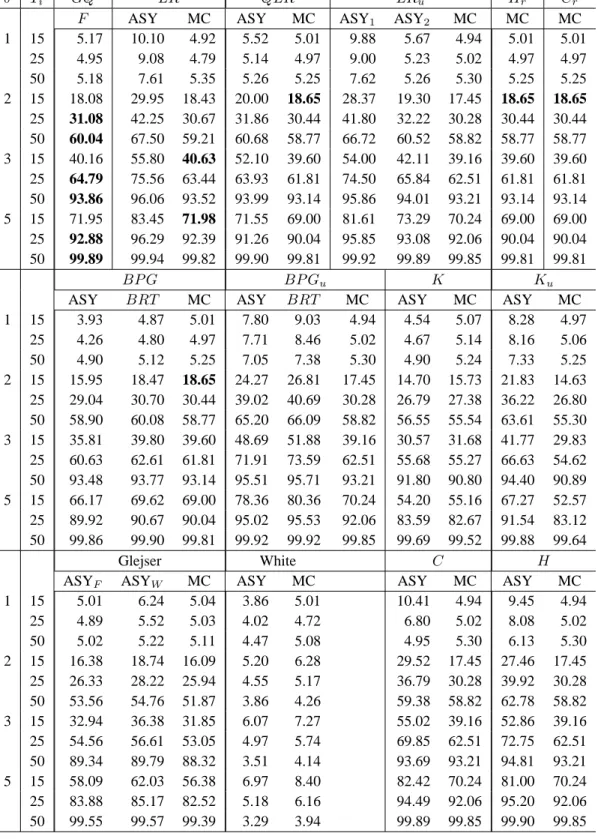
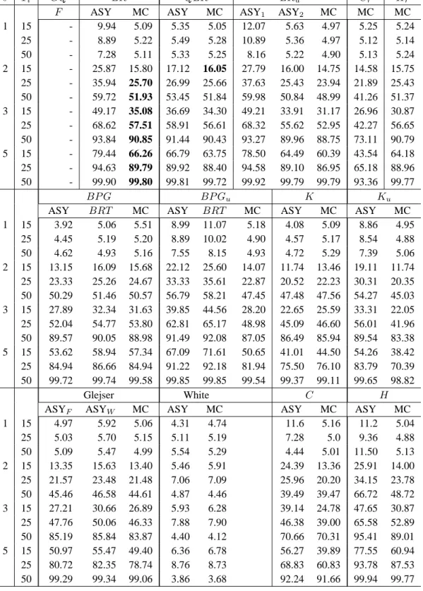
5.2. Tests of variance as a linear function of exogenous variables . . . . 24
5.2.1. Level . . . . 27
5.2.2. Power . . . . 27
5.3. Grouped heteroskedasticity . . . . 27
5.3.1. Level . . . . 28
5.3.2. Power . . . . 28
5.4. Tests for break in variance . . . . 32
List of Propositions
4.1 Proposition : Characterization of pivotal statistics . . . . 15
4.2 Proposition : Pivotal property of residual-based statistics . . . . 16
List of Tables
1 Survey of empirical literature on the use heteroskedasticity tests . . . . 22 Parameter values used for the GARCH models . . . . 19
3 Testing for ARCH and GARCH . . . . 19
4 Empirical size of ARCH-M tests . . . . 20
5 Power of MC ARCH-M tests: normal errors and D1 design . . . . 21
6 Power of MC ARCH-M tests: various error distributions and D2 design . . . . . 22
7 Variance proportional to a regressor . . . . 25
8 Variance as a function of the mean . . . . 26
9 Grouped heteroskedasticity . . . . 29
1.
Introduction
Detecting and making adjustments for the presence of heteroskedasticity in the disturbances of statistical models is one of the fundamental problems of econometric methodology. We study here the problem of testing the homoskedasticity of linear regression disturbances, under parametric (possibly non-Gaussian) distributional assumptions, against a wide range of alternatives, especially in view of obtaining more reliable or more powerful procedures. The heteroskedastic schemes we consider include random volatility models, such as ARCH and GARCH error structures, variances which are functions of exogenous variables, as well as discrete breaks at (possibly unknown) points. The statistical and econometric literatures on testing for heteroskedasticity is quite extensive; for reviews, the reader may consult Judge, Griffiths, Carter Hill, Lütkepohl, and Lee (1985), Godfrey (1988), Pagan and Pak (1993) and Davidson and MacKinnon (1993, Chapters 11 and 16). In linear regression contexts, the most popular procedures include the Goldfeld-Quandt F -test [Goldfeld and Quandt (1965)], Glejser’s regression-type tests [Glejser (1969)], Ramsey’s versions of the Bartlett (1937) test [Ramsey (1969)], the Breusch-Pagan-Godfrey Lagrange multiplier (LM) test [Godfrey (1978), Breusch and Pagan (1979)], White’s general test [White (1980)], Koenker’s studentized test [Koenker (1981)], and Cochran-Hartley-type tests against grouped heteroskedasticity [Cochran (1941), Hartley (1950), Rivest (1986)]; see the literature survey results in Table 1. Other proposed methods include likelihood (LR) tests against specific alternatives [see, for example, Harvey (1976), Buse (1984), Maekawa (1988) or Binkley (1992)] and “robust procedures”, such as the Goldfeld and Quandt (1965) peak test and the procedures suggested by Bickel (1978), Koenker and Bassett (1982) and Newey and Powell (1987).
The above methods do not usually take variances as a primary object of interest, but as nuisance parameters that must be taken into account (and eventually eliminated) when making inference on other model parameters (such as regression coefficients). More recently, in time series contexts and especially financial data analysis, the modeling of variances (volatilities) as a stochastic process has come to be viewed also as an important aspect of data analysis, leading to the current popularity of ARCH, GARCH and other similar models; see Engle (1982, 1995), Engle, Hendry, and Trumble (1985), Bollerslev, Engle, and Nelson (1994), LeRoy (1996), Palm (1996), and Gouriéroux (1997). As a result, detecting the presence of conditional stochastic heteroskedasticity has become an im-portant issue, and a number of tests against the presence of such effects have been proposed; see Engle (1982), Lee and King (1993), Bera and Ra (1995) and Hong and Shehadeh (1999).
Despite the large spectrum of tests available, the vast majority of the proposed procedures are based on large-sample approximations, even when it is assumed that the disturbances are indepen-dent and iindepen-dentically distributed (i.i.d.) with a normal distribution under the null hypothesis. So there has been a number of recent studies that seek to improve the finite-sample reliability of commonly used homoskedasticity tests. In particular, Honda (1988) and Cribari-Neto and Ferrari (1995) de-rived Edgeworth and Bartlett modifications for the Breusch-Pagan-Godfrey criteria, while Cribari-Neto and Zarkos (1998) considered bootstrap versions of the latter procedures. Tests based on the jackknife method have also been considered; see, for example, Giaccotto and Sharma (1988) and Sharma and Giaccotto (1991). In a multi-equations framework, Bewley and Theil (1987) suggested a simulation-based test for a particular testing problem; however, they did not supply a distributional
Table 1. Survey of empirical literature on the use heteroskedasticity tests Heteroskedasticity test used Literature Share Tests for ARCH and GARCH effects 25.3%
Breusch-Pagan-Godfrey-Koenker 20.9% White’s test 11.3% Goldfeld-Quandt 6.6% Glejser’s test 2.9% Hartley’s test 0.3% Other tests 1.9%
Use of heteroskedasticity consistent standard errors 30.3%
Note _ This survey is based on 379 papers published in The Journal of Business and Economic Statistics, The Journal of Applied Econometrics, Applied Economics, the Canadian Journal of Economics, Economics Letters, over the period 1980 -1997. These results were generously provided by Judith Giles.
theory, either exact or asymptotic.
A limited number of provably exact heteroskedasticity tests, for which the level can be con-trolled for any given sample size, have been suggested. These include: (1) the familiar Goldfeld-Quandt F -test and its extensions based on BLUS [Theil (1971)] and recursive residuals [Harvey and Phillips (1974)], which are built against a very specific (two-regime) alternative; (2) a number of procedures in the class introduced by Szroeter (1978), which also include Goldfeld-Quandt-type tests as a special case [see Harrison and McCabe (1979), Harrison (1980, 1981, 1982), King (1981) and Evans and King (1985a)]; (3) the procedures proposed by Evans and King (1985b) and Mc-Cabe (1986). All these tests are specifically designed to apply under the assumption that regression disturbances are independent and identically distributed (i.i.d.) according to a normal distribution under the null hypothesis. Further, except for the Goldfeld-Quandt procedure, these tests require techniques for computing the distributions of general quadratic forms in normal variables such as the Imhof (1961) method, and they are seldom used (see Table 1).
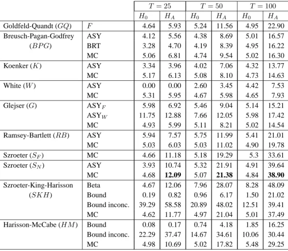
Several studies compare various heteroskedasticity tests from the reliability and power view-points; see, for example, Ali and Giaccotto (1984), Buse (1984), MacKinnon and White (1985), Griffiths and Surekha (1986), Farebrother (1987), Evans (1992), Godfrey (1996), and, in connec-tion with GARCH tests, Engle, Hendry, and Trumble (1985), Lee and King (1993), Sullivan and Giles (1995), Bera and Ra (1995) and Lumsdaine (1995). In addition, most of the references cited above include Monte Carlo evidence on the relative performance of various tests. The main findings that emerge from these studies are the following: (i) no single test has the greatest power against all alternatives; (ii) tests based on OLS residuals perform best; (iii) the actual level of asymptoti-cally justified tests is often quite far from the nominal level: some are over-sized [see, for example, Honda (1988), Ali and Giaccotto (1984) and Binkley (1992)], while others are heavily under-sized, leading to important power losses [see Lee and King (1993), Evans (1992), Honda (1988), Griffiths and Surekha (1986), and Binkley (1992)]; (iv) the incidence of inconclusiveness is high among the bounds tests; (v) the exact tests compare favorably with asymptotic tests but can be quite difficult to
implement in practice. Of course, these conclusions may be influenced by the special assumptions and simulation designs that were considered.
In this paper, we describe a general solution to the problem of controlling the size of ho-moskedasticity tests in linear regression contexts. We consider procedures based on the standard tests as well as several extensions of the latter. Specifically, we focus on the following heteroskedas-tic alternatives: (1) ARCH, GARCH and ARCH-in-mean (ARCH-M) effects; (2) breaks in variance at possibly unknown points; (3) cases where the variance depends on a vector of exogenous vari-ables; (4) the case where the variance is a function of the mean of the dependent variable; (5) grouped heteroskedasticity. We exploit the technique of Monte Carlo (MC) tests [Dwass (1957), Barnard (1963), Jöckel (1986), Dufour and Kiviet (1996, 1998)] to obtain provably exact random-ized analogues of the tests considered. This simulation-based procedure yields an exact test when-ever the distribution of the test statistic does not depend on unknown nuisance parameters (i.e., it is pivotal) under the null hypothesis. The fact that the relevant analytical distributions are quite complicated is not a problem in this context: all we need is the possibility of simulating the relevant test statistic under the null hypothesis. In particular, this covers many cases where the finite-sample distribution of the test statistic is intractable or involves parameters which are unidentified under the null hypothesis, as occurs in the problems studied by Davies (1977, 1987), Andrews and Ploberger (1995), and Hansen (1996). Further the method allows one to consider any error distribution that can be simulated, which of course covers both Gaussian and many non-Gaussian distributions (such as stable distributions).
We show here that all the standard homoskedasticity test statistics considered are indeed piv-otal. In particular, we observe that a large class of residual-based tests for heteroskedasticity [studied from an asymptotic viewpoint by Pagan and Hall (1983)] are pivotal in finite samples, hence allow-ing the construction of finite-sample MC versions of these. In this way, the size of many popular asymptotic procedures, such as the Breusch-Pagan-Godfrey, White, Glejser, Bartlett, and Cochran-Hartley-type tests, can be perfectly controlled for any parametric error distribution (Gaussian or non-Gaussian) specified up to an unknown scale parameter. Tests for which a finite-sample theory has been supplied for Gaussian distributions, such as the Goldfeld-Quandt and various Szroeter-type tests, are extended to allow for non-Gaussian distributions. Further, we show that various bounds procedures that were proposed to deal with intractable finite-sample distributions [e.g., by Szroeter (1978), King (1981) and McCabe (1986)] can be avoided altogether in this way.
Our results also cover the important problem of testing for ARCH, GARCH and ARCH-M effects. In this case, MC tests provide finite-sample homoskedasticity tests against standard ARCH-type alternatives where the noise that drives the ARCH process is i.i.d. Gaussian, and allow one to deal in a similar way with non-Gaussian disturbances. In non-standard test problems, such as the ARCH-M case, we observe that the MC procedure circumvents the unidentified nuisance parameter problem. Further, due to the convenience of MC test methods, we define a number of new test statis-tics and show how they can be implemented. These include: (1) combined Breusch-Pagan-Godfrey tests against a break in the variance at an unknown date (or point); (2) combined Goldfeld-Quandt tests against a variance break at an unspecified point, based on the minimum (sup-type) or the prod-uct of individual p-values; (3) extensions of the classic Cochran (1941) and Hartley (1950) tests, against grouped heteroskedasticity, to the regression framework using pooled regression residuals.
Although the null distributions of many of these tests may be quite difficult to establish in finite samples and even asymptotically, we show that the tests can easily be implemented as finite-sample MC tests.1
To assess the validity of residual-based homoskedasticity tests, Godfrey (1996, section 2) de-fined the notion of “robustness to estimation effects”. In principle, a test is considered robust to estimation effects if the underlying asymptotic distribution is the same irrespective of whether dis-turbances or residuals are used to construct the test statistic. Our approach to residual-based tests departs from Godfrey’s asymptotic framework. As noted earlier, MC homoskedasticity tests are based on a finite-sample distributional theory. Indeed, since the test criteria considered are pivotal under the null hypothesis, we shall be able to control perfectly type I error probabilities whenever the error distribution is specified up to an unknown scale parameter [e.g., the variance], even with non-normal errors. Therefore, the adjustments proposed by Godfrey (1996) or Koenker (1981) are not necessary for controlling size. It is also of interest to note that Breusch and Pagan (1979) rec-ognized the pivotal property of the LM homoskedasticity test which might be exploited to obtain simulation-based cut-off points. Here we provide a clear simulation-based strategy that allows one to control the size of the tests even with a very small number of replications.
The performance of the proposed tests is examined by simulation. The MC studies we consider assess the various tests, assuming a correctly specified model. We do not address the effects on the tests which result from misspecifying the model and/or the testing problem. Our results indicate that the MC versions of the popular tests typically have superior size and power properties.
The paper is organized as follows. Section 2 presents the statistical framework and Section 3 defines the test criteria considered. The Monte Carlo test procedure is described in Section 4. In Section 5, we report the results of the Monte Carlo experiments. Section 6 concludes.
2.
Framework
We consider the linear model
yt = x0tβ + ut, (2.1)
ut = σtεt, t = 1, . . . , T, (2.2)
where xt = (xt1, xt2, . . . , xtk)0, X ≡ [x1, . . . , xT]0 is a full-column rank T × k matrix,
β = (β1, . . . , βk)0is a k × 1 vector of unknown coefficients, σ
1, . . . , σT are (possibly random)
scale parameters, and
ε = (ε1, . . . , εT)0 is a random vector with a completely specified
continuous distribution conditional on X . (2.3)
1For example, the combined test procedures proposed here provide solutions to a number of change-point problems.
For further discussion of the related distributional issues, the reader may consult MacNeill (1978), Shaban (1980), Chu and White (1992), Zivot and Andrews (1992), Andrews (1993) and Hansen (1997)]
Clearly the case where the disturbances are normally distributed is included as a special case. We are concerned with the problem of testing the null hypothesis
H0 : σ2t = σ2, t = 1, . . . , T, for some σ, (2.4)
against the alternative HA: σ2t 6= σ2s, for at least one value of t and s.
The hypothesis defined by (2.1) - (2.4) does not preclude dependence nor heterogeneity among the components of ε. So in most cases of practical interest, one would further restrict the distribution of ε, for example by assuming that the elements of ε are independent and identically distributed (i.i.d.), i.e.
ε1, . . . , εT are i.i.d. according to some given distribution F0, (2.5)
which entails that u1, . . . , uT are i.i.d. with distribution function P[ut≤ v] = F0(v/σ) under H0.
In particular, it is quite common to assume that
ε1, . . . , εT i.i.d.∼ N [0, 1] , (2.6)
which entails that u1, . . . , uT are i.i.d. N [0, σ2] under H0. However, as shown in Section 4, the
normality assumption is not needed for several of our results; in particular, it is not at all required for the validity of MC tests for general hypotheses of the form (2.1) - (2.4), hence, a fortiori, if (2.4) is replaced by the stronger assumption (2.5) or (2.6).
We shall focus on the following special cases of heteroskedasticity (HA), namely:
H1 : GARCH and ARCH-M alternatives;
H2 : σ2t depends monotonically on a linear function zt0α of a vector ztof exogenous variables;
H3 : σ2t is a monotonic function of E(yt) (or |E(yt)|);
H4 : σ2tis the same within p subsets of the data but differs across the subsets; the latter specification
is frequently termed grouped heteroskedasticity. Note that H4may include the hypothesis that
the variance changes discretely at some point in time (which may be specified or not). In most cases, the tests considered are functions of the least squares residuals
b
u = (bu1, . . . , buT)0= y − X bβ (2.7) where bβ = (X0X)−1X0y denotes the ordinary least squares (OLS) estimate of β. We shall also write: b σ2 = 1 T T X t=1 b u2t. (2.8)
3.
Test statistics
As already mentioned, among the numerous tests for heteroskedasticity which have been proposed, they are nowadays quite unevenly used [see Table 1], so we have tried to concentrate on the most
popular procedures and alternatives. Unless stated otherwise, we shall assume in this section that (2.6) holds, even though the asymptotic distributional theory for several of the proposed procedures can be obtained under weaker assumptions. The tests we shall study can be conveniently classified in three (not mutually exclusive) categories: (i) the general class of tests based on an auxiliary re-gression involving OLS residuals and some vector of explanatory variables ztfor the error variance;
(ii) tests against ARCH-type alternatives; (iii) tests against grouped heteroskedasticity. 3.1. Tests based on auxiliary regressions
3.1.1. Standard auxiliary regression tests
To introduce these tests in their simplest form, consider the following auxiliary regressions:
b
u2t = zt0α + wt, t = 1, . . . , T, (3.1)
b
u2t− bσ2= zt0α + wt, t = 1, . . . , T, (3.2)
|but| = zt0α + wt, t = 1, . . . , T, (3.3)
where zt = (1, zt2, . . . , ztm)0 is a vector of m fixed regressors on which σtmay depend, α =
(α1, . . . , αm)0 and wt, t = 1, . . . , T, are treated as error terms.2 The Breusch-Pagan-Godfrey
(BP G) LM criterion [Breusch and Pagan (1979), Godfrey (1978)] may be obtained as the explained
sum of squares (ESS) from the regression associated with (3.1) divided by 2bσ4. The Koenker (K) test statistic [Koenker (1981)] is T times the uncentered R2 from regression (3.2). White’s (W ) test statistic is T times the uncentered R2from regression (3.1) using for ztthe r × 1 observations
on the non redundant variables in the vector xt⊗ xt. These tests can be derived as LM-type tests
against alternatives of the form
HA: σ2t = g(zt0α) (3.4) where g(.) is a twice differentiable function. Under H0 and standard asymptotic regularity
condi-tions, we have:
BP Gasyv χ2(m − 1),
Kasyv χ2(m − 1),
W asyv χ2(r − 1),
where the symbolasyv indicates that the test statistic is asymptotically distributed as indicated (under
H0as T → ∞). The standard F statistic to test α2= . . . = αm = 0 in the context of (3.3) yields
the Glejser (G) test [Glejser (1969)]. Again, under H0and standard regularity conditions,
(T − k)Gasyv χ2(m − 1).
Below, we shall also consider F (m − 1, T − k) distribution as an approximation to the null dis-tribution of this statistic. Honda (1988) has also provided a size-correction formula for the BP G
statistic. White’s test was designed against the general alternative HA. The above version of the
Glejser test is valid for the special case where the variance is proportional to zt0α.
Godfrey (1996) has recently shown that, unless the error distribution is symmetric, the G test is deficient in the following sense. The residual-based test is not asymptotically equivalent to a conformable χ2test based on the true errors. Therefore, the G test may not achieve size control. We will show below that this difficulty is circumvented by our proposed MC version of the test. In the same vein, we argue that from a MC test perspective, choosing the Koenker statistic rather than the
BP G has no incidence on size control. We provide a rigorous justification for the latter arguments
in Section 4.
Tests against discrete breaks in variance at some specified date τ may be applied in the above framework by defining ztas a dummy variable of the form zt= zt(τ ), where
zt(τ ) = (
0, t ≤ τ
1, t > τ . (3.5)
Pagan and Hall (1983, p. 117) provide the relevant special form of the BP G test statistic. We also suggest here extensions of this procedure to the case where the break-date τ is left unspecified, and thus may take any one of the values τ = 1, . . . , T − 1. One may then compute a different test statistic for each one of these possible break-dates. Note the problem of combining inference based on the resulting multiple tests was not solved by Pagan and Hall (1983).
3.1.2. Auxiliary regression tests against an unknown variance breakpoint
Let BP Gτ be the BP G statistic obtained on using zt = zt(τ ), where τ = 1, . . . , T − 1.
When used as a single test, the BP Gτ statistic is significant at level α when BP Gτ ≥ χ2α(1),
or equivalently when Gχ1(BP Gτ) ≤ α, where χ
2
α(1) solves the equation Gχ1[χ
2
α(1)] = α and
Gχ1(x) = P[χ
2(1) ≥ x] is the survival function of the χ2(1) probability distribution. G
χ1(BP Gτ)
is the asymptotic p-value associated with BP Gτ. We propose here two methods for combining the
BP Gτ tests.
The first one rejects H0 when at least one of the p-values for τ ∈ J is sufficiently small, where
J is some appropriate subset of the time interval {1, 2, . . . , T − 1}, such as J = [τ1, τ2] where
1 ≤ τ1 < τ2 ≤ T − 1. In theory, J may be any non-empty subset of {1, 2, . . . , T − 1}. More
precisely, we reject H0 at level α when pvmin(BP G; J) ≤ p0(α; J) where
pvmin(BP G; J) ≡ min{Gχ1(BP Gτ) : τ ∈ J} (3.6) and p0(α; J) is the largest point such that P[pvmin(BP G; J) ≤ p0(α; J)] ≤ α under H0, or
equivalently when Fmin(BP G; J) ≥ Fmin(α; J) where
Fmin(BP G; J) ≡ 1 − min{Gχ1(BP Gτ) : τ ∈ J} (3.7)
and Fmin(α; J) = 1−p0(α; J). In general, to avoid over-rejecting, p0(α; J) should be smaller than
of independent test statistics. Here, it is however clear that the statistics BP Gτ, τ = 1, . . . , T − 1,
are not independent, with possibly a complex dependence structure.
The second method we consider consists in rejecting H0 when the product (rather than the
minimum) of the p-values pv×(BP G; J) ≡
Q
τ ∈J
Gχ(BP Gτ) is small, or equivalently when
F×(BP G; J) ≥ F×(J; α) where
F×(BP G; J) ≡ 1 −
Y
τ ∈J
Gχ1(BP Gτ) (3.8)
and F×(J; α) is the largest point such that P[F×(BP G; J) ≥ F×(J; α)] ≤ α under H0. This
general method of combining p-values was originally suggested by Fisher (1932) and Pearson (1933), again for independent test statistics.3 We also propose here to consider a modified version of F×(BP G; J) based on a subset of the p-values Gχ1(BP Gτ). Specifically, we shall consider a
variant of F×(BP G; J) based on the four smallest p-values:
F×(BP G; bJ(4)) = 1 −
Y
τ ∈ bJ(4)
Gχ1(BP Gτ) (3.9)
where bJ(4) is the set of the four smallest p-values in the series {Gχ1(BP Gτ) : τ = 1, 2, . . . , T −
1}. We shall see later that this modified statistic has better power properties. Implicitly, the
maxi-mal number of p-values retained (four in this case) may be chosen to reflect (prior) knowledge on potential break dates.
We will see below that the technique of MC tests provides a simple way of controlling the size of the tests Fmin(BP G; J), F×(BP G; J) and F×(BP G; bJ(4)), although their finite-sample _ and
even their asymptotic _ distributions may be quite intractable. 3.2. Tests against ARCH-type heteroskedasticity
In the context of conditional heteroskedasticity, artificial regressions provide an easy way to com-pute tests for GARCH effects. Engle (1982) proposed a LM test based on the following framework:
yt = x0tβ + ut, t = 1, . . . , T , ut|t−1 ∼ N (0, σ2t) , σ2t = α0+ q X i=1 αiu2t−i, (3.10) 3
For further discussion of methods for combining tests, the reader may consult Miller (1981), Folks (1984), Savin (1984), Dufour (1989, 1990), Westfall and Young (1993), Gouriéroux and Monfort (1995, Chapter 19), and Dufour and Torrès (1998, 2000).
where |t−1 denotes conditioning of information up to and including t − 1. The hypothesis of ho-moskedasticity may then be formulated as follows:
H0 : α1= · · · = αq= 0. (3.11)
The Engle test statistic is given by T R2, where T is the sample size, R2 is the coefficient of de-termination in the regression of squared OLS residuals bu2
t on a constant and bu2t−i(i = 1, . . . , q) .
Under standard regularity conditions, the asymptotic null distribution of this statistic is χ2(q). Lee (1991) has also shown that the same test is appropriate against GARCH(p, q) alternatives, i.e.
σ2t = α0+ p X i=1 θiσ2t−i+ q X i=1 αiu2t−i, (3.12)
and the null hypothesis is
H0 : α1= · · · = αq= θ1= · · · = θp= 0 .
Lee and King (1993) proposed an alternative (G)ARCH test which exploits the one sided nature of
HA. The test statistic is
LK = ( (T − q) PT t=q+1 £ (bu2 t/bσ2− 1) ¤Pq i=1 b u2 t−i ) / ( T P t=q+1 (bu2 t/bσ2− 1)2 )1/2 (T − q) T P t=q+1 µ q P i=1 b u2 t−i ¶2 − Ã T P t=q+1 µ q P i=1 b u2 t−i ¶!2 1/2 (3.13)
and its asymptotic null distribution is standard normal.4
In this paper, we also consider tests against ARCH-M heteroskedasticity (where the shocks affecting the conditional variance of yt also have an effect on its conditional mean). This model
is an extension of (3.10) which allows the conditional mean to be dependent on the time-varying conditional variance. Formally, the model may be defined as follows:
yt = x0tβ + σtφ + ut, t = 1, . . . , T , ut|t−1 ∼ N (0, σ2t) , σ2t = α0+ q X i=1 αiu2t−i.
Then the LM statistic for homoskedasticity hypothesis (3.11) for given φ is:
LM (φ) = 1 2 + φ2bγ 0V · V0V − φ 2 2 + φ2V 0X(X0X)−1X0V ¸−1 V0bγ (3.14) 4
where bγ is a T × 1 vector with elements
b
γt= [(but/bσ)2− 1] + φbut/bσ
and V is a T × (q + 1) matrix whose t-th row is
Vt= (1 , bu2t−1, . . . , bu2t−q) ;
see Bera and Ra (1995). In this case, under H0, the parameter φ is unidentified. Only the sum of
φ and the intercept (φ + β1) is identifiable under H0, although an “estimate” of φ can be produced
under both the null and the alternative hypotheses. In practice, the latter estimate is substituted for
φ to implement the LM test using a cut-off point from the χ2(q) distribution. Bera and Ra (1995)
also discuss the application of the Davies sup-LM test to this problem and show that this leads to more reliable inference.5 It is clear, however, that the asymptotic distribution required is quite complicated. We will show below that the MC test procedure may be applied to this sup-LM test. The unidentified nuisance parameter is not a problem for implementing the MC version of the test. Indeed, it is easy to see that the statistic’s finite sample null distribution is nuisance-parameter-free. The simulation experiment in Section 5.1 shows that this method works very well in terms of size and power.
3.3. Tests based on grouping
An alternative class of tests assumes that observations can be ordered so that the variance is non-decreasing. In practice, the data are typically sorted according to time or some regressor. In the case of H3, the ranking may be based on byt; yet this choice may affect the finite-sample null distributions
of the test statistics. For further reference, let bu(t), t = 1, . . . , T, denote the OLS residuals obtained
after reordering the observations (if needed).
3.3.1. Goldfeld-Quandt tests against an unknown variance breakpoint
The most familiar test in this class is the Goldfeld and Quandt (1965, GQ) test which involves separating the ordered sample into three subsets and computing separate OLS regressions on the first and last data subsets. Let Ti, i = 1, 2, 3, denote the number of observations in each of these
subsets (T = T1+ T2+ T3). Under (2.1) - (2.6) and H0, the test statistic is
GQ(T1, T3, k) = SS3/(T3− k)
1/(T1− k) (3.15)
5
In a recent paper, Demos and Sentana (1998) have proposed one-sided LM tests for ARCH effects as well as critical values for LR and Wald tests which take into account the one-sided nature of the problem. Similarly, Beg, Silvapulle, and Silvapulle (1998) have introduced a one-sided sup-type generalization of the Bera-Ra test, together with simulation-based cut-off points, because of the untractable asymptotic null distributions involved. For further discussion of the difficult asymptotic distributional issues assiciated with such problems, see also Andrews (1999) and Klüppelberg, Maller, Van De Vyver, and Wee (2000). The MC test method should also prove to be useful with these procedures.
where S1 and S3 are the sum of squared residuals from the first T1 and the last T3 observations
(where k < T1 and k < T3). Under the null, GQ(T1, T3, k) v F (T3 − k, T1 − k). The latter
distributional result is exact provided the ranking index does not depend on the parameters of the constrained model. Setting GF (T3−k,T1−k)(x) = P[F (T3− k, T1− k) ≥ x], we denote
pv[GQ; T1, T3, k] = GF (T3−k,T1−k)[GQ(T1, T3, k)] (3.16)
the p-value associated with GQ(T1, T3, k).
The GQ test is especially relevant in testing for breaks in variance.6To account for an unknown (or unspecified) break-date, we propose here (as for the BPG test) statistics of the form:
Fmin(GQ; K) ≡ 1 − min{pv[GQ; T1, T3, k] : (T1, T3) ∈ K} , (3.17)
F×(GQ; K) ≡ 1 −
Y
(T1,T3)∈K
pv[GQ; T1, T3, k] , (3.18)
where K is any appropriate non-empty subset of
K(k, T ) = {(T1, T3) ∈ Z2 : k + 1 ≤ T1 ≤ T − k − 1 and k + 1 ≤ T3 ≤ T − T1} , (3.19)
the set of the possible subsample sizes compatible with the definition of the GQ statistic. Reason-able choices for K could be K = S1(T, T2, L0, U0) with
S1(T, T2, L0, U0) ≡ {(T1, T3) : L0≤ T1 ≤ U0 and T3 = T − T1− T2 ≥ 0} , (3.20)
where T2represents the number of central observations while L0and U0are minimal and maximal
sizes for the subsamples ( 0 ≤ T2 ≤ T − 2k − 2, L0 ≥ k + 1, U0≤ T − T2− k − 1), or
K = S2(T, L0, U0) = {(T1, T3) : L0 ≤ T1 = T3 ≤ U0} (3.21)
where L0 ≥ k + 1 and U0 ≤ I[T /2]; I[x] is the largest integer less than or equal to x. According
to definition (3.20), {GQ(T1, T3, k) : (T1, T3) ∈ K} defines a set of GQ statistics, such that the
number T2 of central observations is kept constant (although the sets of the central observations
differ across the GQ statistics considered); with (3.21), {GQ(T1, T3, k) : (T1, T3) ∈ K} leads to
GQ statistics such that T1 = T3(hence with different numbers of central observations). As with the
BPG statistics, we also consider
F×(GQ; bK(4)) ≡ 1 −
Y
(T1,T3)∈ bK(4)
pv[GQ; T1, T3, k]
where bK(4)selects the four smallest p-values from the set {pv[GQ; T1, T3, k] : (T1, T3) ∈ K}.
It is clear the null distribution of these statistics may be quite difficult to obtain, even asymptot-ically. We will see below that the level of a test procedure based on any one of these statistics can
6Pagan and Hall (1983, page 177) show that the GQ test for a break in variance and the relevant dummy-variable
be controlled quite easily on using the MC version of these tests. 3.3.2. Generalized Bartlett tests
Under the Gaussian assumption (2.6), the likelihood ratio criterion for testing H0 against H4 is a
(strictly) monotone increasing transformation of the statistic:
LR(H4) = T ln(bσ2) −
p
X
i=1
Tiln(bσ2i) (3.22)
where bσ2 is the ML estimator (assuming i.i.d. Gaussian errors) from the pooled regression (2.1) while bσ2i, i = 1, . . . , p, are the ML estimators of the error variances for the p subgroups [which, due to the common regression coefficients require an iterative estimation procedure]. If one further allows the regression coefficient vectors to differ between groups (under both the null and the alter-native hypothesis), one gets the extension to the linear regression setup of the well-known Bartlett (1937) test for variance homogeneity.7 Note Bartlett (1937) studied the special case where the only regressor is a constant, which is allowed to differ across groups. Other (quasi-LR) variants of the Bartlett test, involving degrees of freedom corrections or different ways of estimating the group variances, have also been suggested; see, for example, Binkley (1992).
In the context of H2, Ramsey (1969) suggested a modification to Bartlett’s test that can be run
on BLUS residuals from ordered observations. Following Griffiths and Surekha (1986), we consider an OLS-based version of Ramsey’s test which involves separating the residuals bu(t), t = 1, . . . , T,
into three disjoint subsets Giwith Ti, i = 1, 2, 3, observations respectively. The test statistic is:
RB = T ln(bσ2) − 3 X i=1 Tiln(bσ2i), (3.23) where b σ2= 1 T T X t=1 b u2(t), bσ2i = 1 Ti X t∈Gi b u2(t).
Under the null, RBasyv χ2(2).
3.3.3. Szroeter-type tests
Szroeter (1978) introduced a wide class of tests. The Szroeter tests are based on statistics of the form eh = Ã X t∈A hteu2t ! / Ã X t∈A e u2t ! (3.24) 7
In this case, the estimated variances are bσ2i = Si/Ti, i = 1, . . . , p, and bσ2 =
Pp
i=1TiSi/T, where Siis the sum
of squared errors from a regression which only involves the observations in the i-th group. This of course requires one to use groups with sufficient numbers of observations.
where A is some non-empty subset of {1, 2, . . . , T } , the eut’s are a set of residuals, the ht’s are
a set of nonstochastic scalars such that hs ≤ htif s < t. Szroeter suggested several special cases
of this statistic (obtained by selecting different weights ht), among which we shall consider the
following ones which are based on the OLS residuals from a single regression [eut= bu(t)] :
SKH = " T X t=1 2(1 − cos πt t + 1) bu 2 (t) # / Ã T X t=1 b u2(t) ! , (3.25) SN = µ 6T T2− 1 ¶1/2Ã PT t=1t bu2(t) PT t=1bu2(t) −T + 1 2 ! , (3.26) SF = T X t=T1+T2+1 b u2(t) / ÃT 1 X t=1 b u2(t) ! ≡ SF(T1, T − T1− T2) . (3.27)
Under the null hypothesis, SN follows a N (0, 1) distribution asymptotically. Exact critical points
for SKH [under (2.6)] may be obtained using the Imhof method. Szroeter recommends the fol-lowing bounds tests. Let h∗L and h∗U denote the bounds for the Durbin and Watson (1950) test corresponding to T + 1 observations and k regressors. Reject the homoskedasticity hypothesis if
SKH > 4 − h∗
L, accept if SKH < 4 − h∗u, and otherwise treat the model as inconclusive. King
(1981) provided revised bounds for use with SKH calculated from data sorted such that, under the alternative, the variances are non-increasing. Harrison (1980, 1981, 1982) however showed there is a high probability that the Szroeter and King bounds tests be inconclusive; in view of this, he derived and tabulated beta-approximate critical values based on the Fisher distribution.
As with the GQ test, the Szroeter’s SF statistic may be interpreted as a variant of the GQ statistic
where the residuals from separate regressions have been replaced by those from the regression based on all the observations, so that S3is replaced by eS3 =
PT t=T1+T2+1ub 2 (t)and S1by eS1= PT1 t=1ub2(t).
Harrison and McCabe (1979) suggested a related test statistic based on the ratio of the sum of squares of a subset of {bu(t), t = 1, . . . , T, } to the total sum of squares:
HM = ÃT 1 X t=1 b u2(t) ! / Ã T X t=1 b u2(t) ! (3.28)
where T1 = I[T /2]. Although the test critical points may also be derived using the Imhof method,
Harrison and McCabe proposed the following bounds test. Let
b∗L = µ 1 +(T − T1)Fα(T − T1, T − k) T − k ¶−1 , (3.29) b∗U = µ 1 +(T − T1− k)Fα(T − T1− k, T1) T − k ¶−1 , (3.30)
where Fα(l1, l2) refers to the level α critical value from the F (l1, l2) distribution. H0 is rejected if
HM < b∗
to the null distribution of the HM statistic have also been suggested. However, as argued in Harrison (1981), the two-moment beta approximation offers little savings in computational cost over the exact tests.
McCabe (1986) proposed a generalization of the HM test to the case of heteroskedasticity occurring at unknown points. The test involves computing the maximum HM criterion over several sample subgroups (of size m). The author suggests Bonferroni-based significance points using the quantiles of the Beta distribution with parameters [m/2, (t − m − k)/2] . McCabe discusses an extension to the case where m is unknown. The proposed test is based on the maximum of the successive differences of the order statistics and also uses approximate beta critical points.
3.3.4. Generalized Cochran-Hartley tests
Cochran (1941) and Hartley (1950) proposed two classic tests against grouped heteroskedasticity (henceforth denoted C and H, respectively) in the context of simple Gaussian location-scale models (i.e., regressions that include only a constant). These are based on maximum and minimum sub-group error variances. Extensions of these tests to the more general framework of linear regressions have been considered by Rivest (1986). The relevant statistics then take the form:
C = max 1≤i≤p(s 2 i)/ p X i=1 s2i , (3.31) H = max 1≤i≤p(s 2 i)/ min1≤i≤p(s2i) , (3.32)
where s2i is the unbiased error variance estimator from the i-th separate regression (1 ≤ i ≤ p). Although critical values have been tabulated for the simple location-scale model [see Pearson and Hartley (1976, pp. 202-203)], these are not valid for more general regression models, and Rivest (1986) only offers an asymptotic justification.
We will see below that the Cochran and Hartley tests can easily be implemented as finite-sample MC tests in the context of the regression model (2.1) - (2.4). Further, it will be easy to use in the same way variants of these tests that may be easier to implement or more powerful than the original procedures. Here we shall study Cochran and Hartley-type tests where the residuals from separate regressions are replaced by the OLS residuals from the pooled regression (2.1), possibly after the data have been resorted according to some exogenous variable. This will reduce the loss in degrees of freedom due to the separate regressions. The resulting test statistics will be denoted Crand HRr
respectively. Clearly, standard distributional theory does not apply to these modified test criteria, but they satisfy the conditions required to implement them as MC tests.
3.3.5. Grouping tests against a mean dependent variance
Most of the tests based on grouping, as originally suggested, are valid for alternatives of the form
H2. A natural extension to alternatives such as H3 involves sorting the data conformably with
b
yt; see Pagan and Hall (1983) or Ali and Giaccotto (1984). However this complicates the
sample following the fitted values of a preliminary regression, we suggest the following variants of the tests. Rather than sorting the data, sort the residuals but, t = 1, . . . , T, following bytand
proceed. Provided the fitted values (by1, . . . , byT)0 are independent of the least-squares residuals
(bu1, . . . , buT)0 under the null hypothesis, as occurs for example under the Gaussian assumption
(2.6), this will preserve the pivotal property of the tests and allow the use of MC tests.
4.
Finite-sample distributional theory
We will now show that all the statistics described in Section 3 have null distributions which are free of nuisance parameters and show how this fact can be used to perform a finite-sample MC test of homoskedasticity using any one of these statistics. For that purpose, we shall exploit the following general proposition.
Proposition 4.1 CHARACTERIZATION OF PIVOTAL STATISTICS. Under the assumptions and notations (2.1) − (2.2), let S(y, X) = (S1(y, X), S2(y, X), . . . , Sm(y, X))0 be any vector of
real-valued statistics Si(y, X), i = 1, . . . , m, such that
S(cy + Xd, X) = S(y, X) , for all c > 0 and d ∈ Rk. (4.1)
Then, for any positive constant σ0 > 0, we can write
S(y, X) = S(u/σ0, X) , (4.2)
and the conditional distribution of S(y, X), given X, is completely determined by the matrix X and the conditional distribution of u/σ0 = ∆ε/σ0given X, where ∆ = diag(σt: t = 1, . . . , T ).
In particular, under H0 in (2.4), we have
S(y, X) = S(ε, X) (4.3)
where ε = u/σ, and the conditional distribution of S(y, X), given X, is completely determined by the matrix X and the conditional distribution of ε given X.
PROOF. The result follows on taking c = 1/σ0and d = −β/σ0, which entails, by (2.1),
cy + Xd = (Xβ + u)/σ0− Xβ/σ0= u/σ0.
Then, using (4.1), we get (4.2), so the conditional distribution of S(y, X) only depends on X and the conditional distribution of u/σ0 given X. The identity u0 = ∆ε follows from (2.2). Finally,
under H0 in (2.4), we have u = ∆ε = σε, hence, on taking σ0 = σ, we get u/σ0 = ε and
S(y, X) = S(ε, X).
It is of interest to note that the representation (4.2) holds under both the general heteroskedastic model (2.1) - (2.2) and the homoskedastic model obtained by imposing (2.4), without any parametric
distributional assumption on the disturbance vector u [such as (2.3)]. Then, assuming (2.3), we see that the conditional distribution of S(y, X), given X, is free of nuisance parameters and thus may be simulated. Of course, the same will hold for any transformation of the components of S(y, X), such as statistics defined as the supremum or the product of several statistics (or p-values).
It is relatively easy to check that all the statistics described in Section 3 satisfy the invariance condition (4.1). In particular, on observing that model (2.1) - (2.2) and the hypothesis (2.4) are invariant to general transformations of y to y∗ = cy + Xd, where c > 0 and d ∈ Rk, on y, it
follows that LR test statistics against heteroskedasticity, such the Bartlett test based on LR(H4)in
(3.22), satisfy (4.1) [see Dagenais and Dufour (1991) and Dufour and Dagenais (1992)], and so have null distributions which are free of nuisance parameters.
For the other statistics, the required results follow on observing that they are scale-invariant functions of OLS residuals. For that purpose, it will be useful to state the following corollary of Proposition 4.1.
Corollary 4.2 PIVOTAL PROPERTY OF RESIDUAL-BASED STATISTICS. Under the assumptions
and notations (2.1) − (2.2), let S(y, X) = (S1(y, X), S2(y, X), . . . , Sm(y, X))0be any vector
of real-valued statistics Si(y, X), i = 1, . . . , m, such that S(y, X) can be written in the form
S(y, X) = S (A(X)y, X) , (4.4)
where A(X) is any n × k matrix (n ≥ 1) such that
A(X)X = 0 (4.5)
and S (A(X)y, X) satisfies the scale-invariance condition
S (cA(X)y, X) = S (A(X)y, X) , for all c > 0 . (4.6)
Then, for any positive constant σ0 > 0, we can write
S(y, X) = S (A(X)u/σ0, X) (4.7)
and the conditional distribution of S(y, X), given X, is completely determined by the matrix X and the conditional distribution of A(X)u/σ0 given X. In particular, under H0 in (2.4), we have
S(y, X) = S (A(X)ε, X) , where ε = u/σ, and the conditional distribution of S(y, X), given X, is completely determined by the matrix X and the conditional distribution of A(X)ε given X.
It is easy to see that the conditions (4.4) - (4.6) are satisfied by any scale-invariant function of the OLS residuals from the regression (2.1), i.e. any statistic of the form S(y, X) = S (ˆu, X) such that S (cˆu, X) = S (ˆu, X) for all c > 0 [in this case, we have A(X) = IT− X(X0X)−1X0]. This
applies to all the tests based on auxiliary regressions described in Section 3.1 as well as the tests against ARCH-type heteroskedasticity [Section 3.2].8 On the other hand, the tests designed against
8
For the case of the Breusch-Pagan test, the fact that the test statistic follows a null distribution free of nuisance parameters has been pointed out by Breusch and Pagan (1979) and Pagan and Pak (1993), although no proof is provided
grouped heteroskedasticity [Section 3.3] involve residuals from subsets of observations. These also satisfy the sufficient conditions of Corollary 4.2 although the A(X) matrix involved is different. For example, for the Goldfeld-Quandt statistic, we have:
A(X) = M (X1) 0 0 0 0 0 0 0 M (X3) (4.8)
where M (Xi) = ITi− Xi(Xi0Xi)−1Xi0, X = [X10, X20, X30]0and Xi is a Ti× k matrix. Note the number n of rows in A(X) can be as large as one wishes so several regressions of this type can be used to compute the test statistic, as done for the combined GQ statistic [see (3.17)].
Let us now make the parametric distributional assumption (2.3). Then we can proceed as follows to perform a finite-sample test based on any statistic, say S0 = S(y, X), whose null distribution
(given X) is free of nuisance parameters. Let G(x) be the survival function associated with S0under
H0, i.e. we assume G : R → [0, 1] is the function such that G(x) = PH0[S0≥ x] for all x, where
PH0 refers to the relevant probability measure (under H0). Without loss of generality, we consider
a right-tailed procedure: H0 rejected at level α when S0 ≥ c(α), where c(α) is the appropriate
critical value such that G[c(α)] = α, or equivalently (with probability 1) when G(S0) ≤ α [i.e.
when the p-value associated with the observed value of the statistic is less than or equal to α]. Now suppose we can generate (by Monte Carlo methods) N i.i.d. replications of the error vector
ε according to assumption (2.3). This leads to N simulated samples and N independent realizations
of the test statistic S1, ... , SN. The associated MC critical region obtains as
b pN(S0) ≤ α (4.9) where b pN(x) = N bGN(x) + 1 N + 1 (4.10) and b GN(x) = N1 N X i=1 1[0,∞)(Si− x), 1A(x) = ( 1, x ∈ A 0, x /∈ A . (4.11)
Then, provided the distribution function of S0induced by PH0under H0is continuous, we have:
PH0[bpN(S0) ≤ α] =I [α(N + 1)]
N + 1 , f or 0 ≤ α ≤ 1 , (4.12)
see Dufour and Kiviet (1998).9 In particular, if N is chosen so that α(N + 1) is an integer, we have:
PH0[bpN(S0) ≤ α] = α . (4.13)
by them. The results given here provide a rigorous justification and considerably extend this important observation.
9
If the distribution of S0was not continuous, then we can write PH0[bpN(S0) ≤ α] ≤ I [α(N + 1)] /(N + 1) , so the
procedure described here will be conservative. Under the assumption (2.3), however, the statistics described in section 3 have continuous null distributions.
Thus the critical region (4.9) has the same size as the critical region G(S0) ≤ α.
The MC test so obtained is theoretically exact, irrespective of the number N of replications used. Note that the procedure is closely related to the parametric bootstrap, with however a fundamental difference: bootstrap tests are, in general, provably valid for N → ∞. See Dufour and Kiviet (1996, 1998), Kiviet and Dufour (1997) and Dufour and Khalaf (2001) for some econometric applications of MC tests.
Finally, it is clear from the statement of Assumption (2.3) that normality does not play any role for the validity of the MC procedure just described. So we can consider in this way alternative error distributions such as heavy-tailed distributions like the Cauchy distribution. The only tests for which normality may play a central role in order to control size are those designed against a variance which is a function of the mean and where the least squares (LS) residuals are sorted according to the LS fitted values byt, t = 1, . . . , T. Since the distribution of the latter depends on nuisance parameters
(for example, the regression coefficients β), it is not clear that a test statistic which depends on both
b
u = (bu1, . . . , buT)0and by = (by1, . . . , byT)0will have a null distribution free of nuisance parameters
under the general distributional assumption (2.3). However, if we make the Gaussian assumption (2.6), bu and by are mutually independent under H0, and we can apply the argument justifying the
MC test procedure conditional on by.
5.
Simulation experiments
In this section, we present simulation results illustrating the performance of the procedures de-scribed in the preceding sections. Because the number of tests and alternative models is so large, we have gathered our results in four groups corresponding to four basic types of alternatives: (1) GARCH-type heteroskedasticity; (2) variance as a linear function of exogenous variables; (3) grouped heteroskedasticity; (4) variance break at a (possibly unspecified) point.
5.1. Tests for ARCH and GARCH effects
For ARCH and GARCH alternatives, our simulation experiment was based on the following speci-fication: yt = x0tβ + εth 1 2 t + htφ , (5.14) ht = ω0+ ¡ α0ε2t−1+ α1 ¢ ht−1 , t = 1, . . . , T, (5.15)
where xt is defined as in (2.1), and εt iid∼ N (0, 1) , t = 1, . . . , T. We took T = 25, 50, 100
and k = I[T1/2] + 1. In the case of tests against ARCH-M alternatives [experiment (iv)], we also considered a number of alternative error distributions, according to the examples studied by Godfrey (1996): N (0, 1), χ2(2), U [−.5, .5], t(5) and Cauchy.
The data were generated setting β = (1, 1, . . . , 1 )0and ω0 = 1. In this framework, the model
with φ = 0 and α1 = 0 is a standard ARCH(1) specification, while φ = 0 yields a GARCH(1,1)
model. The ARCH-M system discussed in Bera and Ra (1995) corresponds to α1 = 0. The
Table 2. Parameter values used for the GARCH models Experiment φ α0 α1 (i) 0 0 0 (ii) 0 .1, .5, .9, 1 0 (iii) 0 .1 .5 0 .25 .65 0 .4 .5 0 .15 .85 0 .05 .95 (iv) −2, −1, 1, 2 0, .1 , .5, .9 0
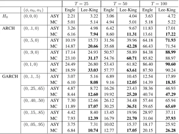
Table 3. Tests against ARCH and GARCH heteroskedasticity
T = 25 T = 50 T = 100
(φ, α0, α1) Engle Lee-King Engle Lee-King Engle Lee-King
H0 (0, 0, 0) ASY 2.21 3.22 3.06 4.04 3.63 4.72 MC 5.01 5.14 4.94 5.01 5.18 5.22 ARCH (0, .1, 0) ASY 3.26 4.98 6.42 9.67 11.83 17.01 MC 6.16 7.94 8.60 11.31 13.61 17.22 (0, .5, 0) ASY 10.19 15.73 31.56 39.96 64.18 71.93 MC 14.87 20.66 35.68 42.28 66.43 71.54 (0, .9, 0) ASY 17.14 24.93 50.57 58.89 84.38 88.99 MC 23.10 31.17 54.76 60.71 85.82 88.97 (0, 1, 0) ASY 24.49 26.80 53.43 61.82 86.40 90.60 MC 18.59 33.03 57.77 63.61 87.50 90.24 GARCH (0, .1, .5) ASY 3.07 5.16 6.89 10.45 12.54 17.89 MC 6.10 8.08 9.16 12.05 14.39 18.35 (0, .25, .65) ASY 4.87 8.72 16.26 23.43 38.36 46.93 MC 8.44 12.60 19.92 25.20 40.74 47.29 (0, .40, .50) ASY 7.30 12.66 26.12 34.48 57.44 65.94 MC 11.89 17.07 30.25 36.51 59.65 65.69 (0, .15, .85) ASY 4.42 8.40 13.45 19.96 28.97 37.11 MC 7.93 12.39 16.79 21.70 31.04 37.93 (0, .05, .95) ASY 3.75 7.31 10.02 15.37 18.17 25.92 MC 6.84 10.74 12.77 17.05 20.15 26.28
Note: In this table as well as in the subsequent ones, the rejection frequencies are reported in percentages.
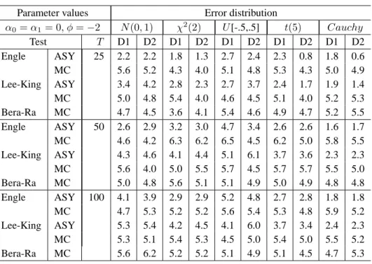
Table 4. Empirical size of ARCH-M tests
Parameter values Error distribution
α0= α1= 0, φ = −2 N (0, 1) χ2(2) U [-.5,.5] t(5) Cauchy Test T D1 D2 D1 D2 D1 D2 D1 D2 D1 D2 Engle ASY 25 2.2 2.2 1.8 1.3 2.7 2.4 2.3 0.8 1.8 0.6 MC 5.6 5.2 4.3 4.0 5.1 4.8 5.3 4.3 5.0 4.9 Lee-King ASY 3.4 4.2 2.8 2.3 2.7 3.7 2.4 1.7 1.9 1.4 MC 5.0 4.8 5.4 4.0 4.6 4.5 5.1 4.0 5.2 5.3 Bera-Ra MC 4.7 4.5 3.6 4.1 5.4 4.6 4.9 4.7 5.2 5.5 Engle ASY 50 2.6 2.9 3.2 3.0 4.7 3.4 2.6 2.6 1.6 1.7 MC 4.6 4.2 6.3 6.2 6.5 4.5 6.2 5.0 5.8 5.5 Lee-King ASY 4.3 4.6 4.1 4.4 5.1 6.1 3.7 3.6 2.3 2.3 MC 5.6 4.0 5.0 5.5 5.7 4.5 5.7 5.7 5.5 5.0 Bera-Ra MC 5.0 4.8 5.6 5.1 5.1 4.9 5.0 4.9 4.8 4.8 Engle ASY 100 4.1 3.9 2.9 2.9 5.2 4.8 2.7 2.8 1.8 1.8 MC 4.7 5.3 5.2 5.2 5.6 5.4 5.3 4.8 5.9 5.2 Lee-King ASY 5.3 5.4 4.2 4.5 4.1 6.0 3.7 3.4 2.4 2.3 MC 5.3 5.1 5.4 5.3 4.5 5.0 5.4 5.0 5.5 5.2 Bera-Ra MC 5.6 6.2 5.2 5.2 5.1 4.9 5.1 4.5 4.7 5.3
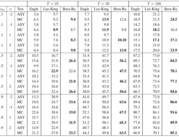
Table 5. Power of MC ARCH-M tests: normal errors and D1 design
T = 25 T = 50 T = 100
α0 φ Test Engle Lee-King Bera-Ra Engle Lee-King Bera-Ra Engle Lee-King Bera-Ra
.1 -2 ASY 3.6 5.7 7.7 9.5 16.0 21.2 MC 6.3 9.2 9.4 9.5 13.9 12.6 18.5 21.5 24.5 .1 -1 ASY 3.8 5.7 6.7 9.8 14.2 18.6 MC 6.4 8.9 8.7 8.4 11.9 9.8 16.0 18.2 16.4 .1 1 ASY 3.8 5.4 6.9 9.7 13.5 17.8 MC 5.9 7.6 8.3 8.2 10.9 10.10 15.1 17.1 17.1 .1 2 ASY 3.8 5.4 7.8 11.3 15.4 21.0 MC 6.4 8.4 9.0 9.8 12.5 13.0 17.5 20.6 23.9 .5 -2 ASY 10.5 16.7 31.4 41.7 67.2 73.0 MC 15.6 21.9 26.4 36.5 43.6 56.2 69.1 72.7 84.5 .5 -1 ASY 9.9 17.1 33.5 42.9 68.3 76.3 MC 16.2 22.9 22.6 38.5 45.2 47.5 70.5 75.6 78.1 .5 1 ASY 10.2 15.2 32.4 41.5 64.8 74.8 MC 14.4 19.6 21.0 36.8 43.2 46.2 67.0 73.4 77.1 .5 2 ASY 10.4 16.6 34.4 43.8 63.3 72.5 MC 16.0 22.4 26.6 38.0 45.3 56.6 66.3 70.9 84.6 .9 -2 ASY 13.3 20.9 41.0 49.7 67.6 72.8 MC 19.6 24.7 33.6 45.6 50.6 63.6 69.4 72.6 86.6 .9 -1 ASY 16.4 24.6 46.7 56.4 79.3 84.2 MC 22.6 30.6 33.0 52.1 58.8 67.5 80.7 84.1 91.6 .9 1 ASY 15.7 23.7 47.0 56.6 75.7 81.5 MC 21.3 29.5 31.9 51.2 58.1 65.3 77.6 82.0 89.9 .9 2 ASY 14.9 22.9 40.7 48.3 65.9 70.4 MC 21.2 27.0 33.3 44.3 49.8 63.5 66.9 70.1 85.1