Approximating Likelihood Ratios with Calibrated Discriminative Classifiers

(1)

Approximating Likelihood Ratios with

Calibrated Discriminative Classifiers

Kyle Cranmer

1

, Juan Pavez

2

, and Gilles Louppe

1

_{New York University}

2

_{Federico Santa Mar´ıa University}

March 21, 2016

Abstract

In many fields of science, generalized likelihood ratio tests are established tools for statistical inference. At the same time, it has become increasingly common that a simulator (or generative model) is used to describe complex processes that tie pa-rameters θ of an underlying theory and measurement apparatus to high-dimensional observations x ∈ Rp. However, simulator often do not provide a way to evaluate the likelihood function for a given observation x, which motivates a new class of likelihood-free inference algorithms. In this paper, we show that likelihood ratios are invariant under a specific class of dimensionality reduction maps Rp 7→ R. As a di-rect consequence, we show that discriminative classifiers can be used to approximate the generalized likelihood ratio statistic when only a generative model for the data is available. This leads to a new machine learning-based approach to likelihood-free inference that is complementary to Approximate Bayesian Computation, and which does not require a prior on the model parameters. Experimental results on artifi-cial problems with known exact likelihoods illustrate the potential of the proposed method.

Keywords: likelihood ratio, likelihood-free inference, classification, particle physics, surro-gate model

(2)

1 Introduction

The likelihood function is the central object that summarizes the information from an ex-periment needed for inference of model parameters. It is key to many areas of science that report the results of classical hypothesis tests or confidence intervals using the (generalized or profile) likelihood ratio as a test statistic. At the same time, with the advance of comput-ing technology, it has become increascomput-ingly common that a simulator (or generative model) is used to describe complex processes that tie parameters θ of an underlying theory and measurement apparatus to high-dimensional observations x. However, directly evaluating the likelihood function in these cases is often impossible or is computationally impractical. The main result of this paper is to show that the likelihood ratio is invariant under

dimensionality reductions Rp 7→ R, under the assumption that the corresponding

transfor-mation is itself monotonic with the likelihood ratio. As a direct consequence, we derive and propose an alternative machine learning-based approach for likelihood-free inference that can also be used in a classical (frequentist) setting where a prior over the model pa-rameters is not available. More specifically, we demonstrate that discriminative classifiers can be used to construct equivalent generalized likelihood ratio test statistics when only a generative model for the data is available for training and calibration.

As a concrete example, let us consider searches for new particles at the Large Hadron Collider (LHC). The simulator that is sampling from p(x|θ) is based on quantum field theory, a detailed simulation of the particle detector, and data processing algorithms that transform raw sensor data into the feature vector x (Sjostrand et al., 2006; Agostinelli et al., 2003). The ATLAS and CMS experiments have published hundreds of papers where the final result was formulated as a hypothesis test or confidence interval using a general-ized likelihood ratio test (Cowan et al., 2010), including most notably the discovery of the

(3)

Higgs boson (The ATLAS Collaboration, 2012; The CMS Collaboration, 2012) and sub-sequent measurement of its properties. The bulk of the likelihood ratio tests at the LHC are based on the distribution of a single event-level feature that discriminates between a hypothesized process of interest (labeled signal ) and various other processes (labeled back-ground ). Typically, data generated from the simulator are used to approximate the density at various parameter points, and an interpolation algorithm is used to approximate the parameterized model (Cranmer et al., 2012). In order to improve the statistical power of these tests, hundreds of these searches have already been using supervised learning to train classifiers to discriminate between two two discrete hypotheses based on a high dimensional feature vector x. The results of this paper outline how to extend the use of discriminative classifiers for composite hypotheses (parameterized by θ) in a way that fits naturally into the established likelihood based inference techniques.

The rest of the paper is organized as follows. In Sec. 2, we first introduce the likelihood ratio test statistic in the setting of simple hypothesis testing, and then outline how it can be computed exactly using calibrated classifiers. In Sec. 3, we generalize the proposed ap-proach to the case of composite hypothesis testing and discuss directions for approximating the statistic efficiently. We then illustrate the proposed method in Sec. 4 and outline how it could improve statistical analysis within the field of high energy physics. Related work and conclusions are finally presented in Sections 5 and 6.

(4)

2 Likelihood ratio tests

2.1 Simple hypothesis testing

Let X be a random vector with values x ∈ X ⊆ Rp and let pX(x|θ) denote the density

probability of X at value x under the parameterization θ. Let also assume i.i.d. observed

data D = {x1, . . . , xn}. In the setting where one is interested in simple hypothesis testing

between a null θ = θ0 against an alternate θ = θ1, the Neyman-Pearson lemma states that

the likelihood ratio

λ(D; θ0, θ1) = Y x∈D pX(x|θ0) pX(x|θ1) (2.1) is the most powerful test statistic.

In order to evaluate λ(D), one must be able to evaluate the probability densities pX(x|θ0)

and pX(x|θ1) at any value x. However, it is increasingly common in science that one has a

complex simulation that can act as generative model for pX(x|θ), but one cannot evaluate

the density directly. For instance, this is the case in high energy physics (Neal, 2007) where the simulation of particle detectors can only be done in the forward mode.

2.2 Approximating likelihood ratios with classifiers

The main result of this paper is to generalize the observation that one can form a test statistic λ0(D; θ0, θ1) = Y x∈D pU(u = s(x)|θ0) pU(u = s(x)|θ1) (2.2) that is strictly equivalent to 2.1, provided the change of variable U = s(X) is based on a (parameterized) function s that is strictly monotonic with the density ratio

r(x; θ0, θ1) =

pX(x|θ0) pX(x|θ1)

(5)

As derived below, this allows to recast the original likelihood ratio test into an alternate form in which supervised learning can be used to build s(x) as a discriminative classifier. In Sec. 3 we extend this result to generalized likelihood ratio tests, where it will be useful

to have the classifier decision function s parameterized in terms of (θ0, θ1).

Theorem 1. Let X be a random vector with values in X ⊆ Rp and parameterized probability

density pX(x = (x1, ..., xp)|θ) and let s : Rp 7→ R be a function monotonic with the density

ratio r(x; θ0, θ1), for given parameters θ0 and θ1. In these conditions,

r(x; θ0, θ1) = pX(x|θ0) pX(x|θ1) = pU(u = s(x)|θ0) pU(u = s(x)|θ1) , (2.4)

where pU(u = s(x; θ0, θ1)|θ) is the induced probability density of U = s(X; θ0, θ1).

Proof. Starting from the definition of the probability density function, we have

pU(u = s(x)|θ0) = d du Z {x0_:s(x0_)≤u} pX(x0|θ0)dx0 = Z Rp δ(u − s(x0))pX(x0|θ0)dx0 (2.5)

Intuitively, this expression can be understood as the integral over all x0 _{∈ R}p _{such that}

s(x0) = u, as picked by the Dirac δ function. Given Theorem 6.1.5 of H¨ormander (1990),

it further comes pU(u = s(x)|θ0) = Z x0_∈Ω u 1 |∇s(x0_)|pX(x 0_|θ 0)dSx0 (2.6) where Ωu = {x0 : s(x0) = u}, |∇s(x0)| = q Pp i=1| ∂ ∂xis(x 0_)|2 _{and where dS} x0 is the Euclidean

surface measure on Ωu. Also, since s(x) is monotonic with r(X; θ0, θ1), there exists an

invertible function m : R+_{7→ R such that s(x) = m(r(X; θ}

0, θ1)). In particular, we have

pX(x|θ0) pX(x|θ1)

= m−1(s(x))

(6)

Similarly, Equation 2.6 can be used to derive pU(u = s(x)|θ1), finally yielding

In light of this result, the likelihood ratio estimation problem can now be recast as a (probabilistic) classification problem, by noticing that the decision function

s∗(x) = pX(x|θ1)

pX(x|θ0) + pX(x|θ1)

. (2.10)

modeled by a classifier trained to distinguish samples x ∼ pθ0 from samples x ∼ pθ1

satisfies the conditions of Thm. 1 (see Appendix A). In other words, supervised learning yields a sufficient procedure for Thm. 1 to hold, guaranteeing that any universally strongly

consistent algorithm can be used for learning s∗. Note however, that it is not a necessary

procedure since Thm. 1 holds for any monotonic function m of the density ratio, not only

(7)

classifier s(x) which is imperfect up to a monotonic transformation of r(x), then one can still

resort to calibration (i.e., modeling pU(u = s(x))) to compute r(x) exactly. For this reason,

the proposed method is expected to be more robust than directly using (1 − s(x))/s(x) as

an approximate of r(x) (which indeed converges towards r(x) when s(x) tends to s∗(x)).

2.3 Learning and calibrating s

In order for the proposed approach to be useful in the likelihood-free setting, we need to

be able to approximate both s(x) and p(s(x)|θ) based on a finite number of samples {xi}

drawn from the generative model p(x|θ).

As outlined above, any consistent probabilistic classification algorithm can be used for

learning an approximate map ˆs(x) of Eqn. 2.10. In the common case where the density

ratio is expected to smoothly vary around x, we would however recommend learning models

whose output value ˆs(x) also smoothly varies around x, such as neural networks. For small

training sets, tree-based methods are not expected to work so well for this use case, since

they usually model ˆs(x) as a non-strictly monotonic composition of step functions. In such

cases where ˆs(x) is not monotonic with r(x), the induced probability does not factorize

as in Eqn. 2.8, leading to artifacts in the resulting approximation of the density ratio. Provided enough training data, accurate results can however still be achieved, given the universal approximator capacity of tree-based models.

Given a reduction map s, our results show that a statistic equivalent to the likelihood ratio can be constructed, provided p(s(x)|θ) can be evaluated. Again, we do not have

a direct and exact way for evaluating this density, but an approximation ˆp(ˆs(x)|θ) can

be built instead, e.g. using density estimation algorithms, such as histograms or kernel

density estimation applied to {ˆs(xi)}, where the {xi} are drawn from the generative model.

(8)

learning p(x|θ), since the reduction s projects x into a one-dimensional space in which only the (simpler) informative content of r(x) is preserved.

An alternative approach for calibration is to approximate the density ratio r(ˆs(x))

directly. For example, isotonic regression, which is commonly used to transform the

clas-sifier score ˆs(x) into ˆsiso(x) that more accurately reflect the posterior probability s∗(x)

of Eqn. 2.10, can be used for calibration. This is done by inverting the relationship

r(x) = (1 − s∗(x))/s∗(x) to obtain ˆr(ˆs(x)) = (1 − ˆsiso(x))/ˆsiso(x). Additionally, Sec. 5

describes related work in which the ratio ˆr(x) is estimated directly on the feature space X .

One strength of the proposed approach is that it factorizes the approximation of the

di-mensionality reduction (ˆs(x) ≈ s(x)) from the calibration procedure (ˆp(ˆs(x)|θ) ≈ p(ˆs(x)|θ)

or ˆr(ˆs(x)) ≈ r(ˆs(x))). Thus, even if the classifier does a poor job at learning the optimal

decision function 2.10 and, therefore, at reproducing the level sets of the per-sample

likeli-hood ratio, the density of ˆs can still be well calibrated. In that case, one might loose power,

but the resulting inference will still be valid. This point was made by Neal (2007) and is well appreciated by the particle physics community that typically takes a conservative at-titude towards the use of machine learning classifiers precisely due to concerns about the calibration of p-values in the face of nuisance parameters associated to the simulator.

3 Generalized likelihood ratio tests

Thus far we have shown that the target likelihood ratio r(x; θ0, θ1) with high dimensional

features x can be reproduced via the univariate densities p(s(x)|θ0) and p(s(x)|θ1) if the

reduction s(x) is monotonic with r(x; θ0, θ1). We now generalize from the ratio of two

simple hypotheses specified by θ0 and θ1 to the case of composite hypothesis testing where

(9)

3.1 Composite hypothesis testing

In the case of composite hypotheses θ ∈ Θ0 against an alternative θ ∈ Θ1 (such that

Θ0 ∩ Θ1 = ∅ and Θ0 ∪ Θ1 = Θ), the generalized likelihood ratio test, also known as the

profile likelihood ratio test, is commonly used

Λ(Θ0) =

sup_θ∈Θ₀p(D|θ)

sup_θ∈Θp(D|θ) . (3.1)

This generalized likelihood ratio can be used both for hypothesis tests in the presence of nuisance parameters or to create confidence intervals with or without nuisance parame-ters. Often, the parameter vector is broken into two components θ = (µ, ν), where the µ components are considered parameters of interest while the ν components are considered

nuisance parameters. In that case Θ0 corresponds to all values of ν with µ fixed.

Evaluating the generalized likelihood ratio as defined by Eqn. 3.1 requires finding for both the numerator and the denominator the maximum likelihood estimator

ˆ

θ = arg max θ

p(D|θ). (3.2)

Again, this is made difficult in the likelihood-free setting and it is not obvious that we can find the same estimators if we are working instead with p(s(x)|θ). Fortunately, there is a construction based on s that works: the maximum likelihood estimate of Eqn. 3.2 is the

same as the value that maximizes the likelihood ratio with respect to p(D|θ1), for some

(10)

where s(x; θ, θ1) denotes a parameterized transformation s of X in terms of (θ, θ1) that

is monotonic with r(x; θ, θ1). Note that it is important that we include the denominator

p(s(x; θ, θ1)|θ1) because this cancels Jacobian factors that vary with θ.

Finally, once the maximum likelihood estimates have been found for both the numerator and denominator of Eqn. 3.1, the generalized likelihood ratio can be estimated as outlined in Sec. 2.2 for simple hypothesis testing.

3.2 Parameterized classification

In order to provide parameter inference in the likelihood-free setting as described above,

we must train a family s(x; θ0, θ1) of classifiers parameterized by θ0 and θ1, the parameters

associated to the null and alternate hypotheses, respectively. While this could be done

independently for all θ0 and θ1, using the procedure outlined in Sec. 2, it is desirable

and convenient to have a smooth evolution of the classification score as a function of the parameters. For this reason, we anticipate a single learning stage based on training data

with input (x, θ0, θ1)iand target yi, as outlined in Alg. 1. Somewhat unusually, the unknown

values of the parameters are taken as input to the classifier; their values will be specified via the enveloping (generalized) likelihood ratio of Eqn. 3.1. In this way, the parameterized

classifier now models the distribution of the output y conditional to (x, θ0, θ1), for any x

(11)

Algorithm 1 Learning a parameterized classifier. T := {}; while size(T ) < N do Draw θ0 ∼ πΘ0; Draw x ∼ p(x|θ0); T := T ∪ {((x, θ0, θ1), y = 0)}; Draw θ1 ∼ πΘ1; Draw x ∼ p(x|θ1); T := T ∪ {((x, θ0, θ1), y = 1)}; end while

Learn a single classifier s(x; θ0, θ1) from T .

While the optimal decision function 2.10 is expected to be learned for the parameter

values θ0 and θ1 selected in Alg. 1, it is not clear whether the optimal decision function can

be expected for data generated from θ₀0 and θ₁0 never jointly encountered during learning.

Similarly, it is not clear how the limited capacity of the classifier may impact the perfor-mance of the resulting parameterized decision function. Preliminary exploration by Baldi et al. (2016) shows that a uniform grid scan over parameter space is an effective practical

approach; however, we introduce the distributions πΘ0 and πΘ1 into the Alg. 1 to allow for

a more sophisticated sampling strategy.

3.3 Parameterized calibration

Once the parameterized classifier ˆs(x; θ0, θ1) is trained, we can use the generative model

together with one of the calibration strategies discussed in Sec. 2.3 for particular values of

(12)

problem. The challenge comes from the need to calibrate this density for all values of θ. A straightforward approach would be to run the generative model on demand for any particular value of θ. In the context of a likelihood fit this would mean that the optimization algorithm that is trying to maximize the likelihood with respect to θ needs access to the generative model p(x|θ). This is the strategy used for the examples presented in Sec. 4.

Calibrating the density on-demand can be impractical when the generative model is computationally expensive or has high-latency (for instance some human intervention is required to reconfigure the generative model). In high energy physics, where it is common to calibrate the distribution of a fixed classifier. There the strategy is to interpolate the distribution between discrete values of θ in order to produce a continuous parameterization for p(s|θ) (Read, 1999; Cranmer et al., 2012; Baak et al., 2015). One can easily imagine a number of approaches to parameterized calibration and the relative merits of those ap-proaches will depend critically on the dimensionality of θ and the computational cost of the generative model. We leave a more general strategy for this overarching optimization problem as an area of future work.

3.4 Mixture models

In the special case of (simple or composite) hypothesis testing between models defined as known mixtures of several components, i.e. when p(x|θ) can be written as

p(x|θ) =X

c

(13)

the target likelihood ratio can be formulated in terms of pairwise classification problems. Specifically, we can write

The second line is a trivial, but a useful decomposition into pairwise density ratio

sub-problems between pc0(x|θ₁) and p_c(x|θ₀). The third line uses Thm. 1 to relate the

high-dimensional likelihood ratio into an equivalent calibrated likelihood ratio based on the univariate density of the corresponding classifier.

In applications where mixture models are commonly used, this decomposition allows

one to construct better likelihood ratio estimates since it allows the classifiers sc,c0 to focus

on simpler sub-problems, for which higher accuracy is expected.

Finally, as a technical point, in the situation where the only free parameters of the model

are the mixture coefficients wc, the distributions pc(sc,c0(x; θ₀, θ₁)|θ) are independent of θ.

For this reason, sub-ratios rc,c0(x; θ₀, θ₁) =

pc0(sc,c0(x;θ0,θ1)|θ1)

pc(sc,c0(x;θ0,θ1)|θ0) simplify to

pc0(sc,c0(x))

pc(sc,c0(x)), which can

be pre-computed without the need of parameterized classification or calibration.

3.5 Diagnostics

While Thm. 1 states that the likelihood ratio r(x; θ0, θ1) is invariant under the

dimension-ality reduction s(x; θ0, θ1) provided that it is monotonic with r(x; θ0, θ1) itself and we know

that any universally strongly consistent algorithm can be used to learn such a function,

(14)

some diagnostic procedures to assess the quality of this approximation. This is complicated by the fact that in the likelihood-free setting, we don’t have access to the true likelihood ratio. Below we consider two such diagnostic procedures that can be implemented in the likelihood-free setting. We illustrate these diagnostic procedures in Fig. 5.

The first diagnostic procedure is related to the procedure for finding the MLE ˆθ in

Eqn. 3.3. As pointed out there it is important that one maximizes the likelihood ratio as the surface integral and Jacobian factors related to the dimensionality reduction only cancel in the ratio (see Eqn. 2.8). Importantly, they also only cancel if the reduction map satisfies

the assumptions of Thm. 1. Moreover, the resulting value of ˆθ should be independent of

the value of θ1 used in the denominator of the likelihood ratio. Similarly, we have

log Λ(θ) = log p(D|θ) p(D|ˆθ) = log p(D|θ) p(D|θ1) − log p(D|ˆθ) p(D|θ1) (3.6)

for all values of θ1. Thus, by explicitly checking the independence of these quantities on θ1

we indirectly probe the quality of the approximation ˆr(ˆs(x; θ0, θ1)) ≈ r(s(x; θ0, θ1)).

The second diagnostic procedure leverages the connection of this technique to direct density ratio estimation and its application to covariate shift and importance sampling.

The idea is simple: we test the relationship p(x|θ0) = p(x|θ1)r(s(x; θ0, θ1)) with the

ap-proximate ratio ˆr(ˆs(x; θ0, θ1)) and samples drawn from the generative model. More

specif-ically, we can train a classifier to distinguish between unweighted samples from p(x|θ0)

and samples from p(x|θ1) weighted by ˆr(ˆs(x; θ0, θ1)). If the classifier can distinguish

be-tween the distributions, then ˆr(ˆs(x; θ0, θ1)) is not a good approximation of r(s(x; θ0, θ1)).

In contrast, if the classifier is unable to distinguish between the two distributions, then

either ˆr(ˆs(x; θ0, θ1)) is a good approximation or the discriminator is not effective. The two

situations can be disentangled to some degree by training another classifier to distinguish

(15)

4 Examples and applications

In this section, we illustrate the proposed method on two representative examples where the exact likelihood is known and then discuss its application to high energy physics. The code used to produce the results and extended details for these examples is available in Ref. (Louppe et al., 2016), which utilizes the classification and calibration routines in scikit-learn (Pedregosa et al., 2011).

4.1 Likelihood ratios of mixtures of normals

As a simple and illustrative example, let us first consider the approximation of the log-likelihood ratio log (r(x; γ = 0.05, γ = 0)) between the 1D mixtures p(x|γ = 0.05) and p(x|γ = 0) defined as p(x|γ) = (1 − γ)pc0(x) + pc1(x) 2 + γ pc2(x), (4.1) where pc0 := N (µ = −2, σ 2 _{= 0.25}2_{), p} c1 := N (µ = 0, σ 2 _{= 4), p} c2 := N (µ = 1, σ 2 _{= 0.25).}

Samples drawn for the nominal value γ = 0.05 are shown in Figure 1a and used later for inference.

Figure 1b shows the intermediate stages for the decomposition described in Sec. 3.4.

The blue and green curves show pc0(ˆs_c,c0(x)), the distributions for the score for the

sub-classifiers for the three pair-wise comparisons of the mixture components. The red curves

in Fig. 1b show the approximation of the density ratio (rescaled as (1 + ˆr(x))−1) obtained

from those distributions.

Figures 1c and 1d show the approximate log ˆr(x) as a function of x using a 2-layer

neural network and a random forest for the classifier ˆs(x). The neural network provides

(16)

decision function is piece-wise constant. The blue curves show the exact log r(x), the green

curves show log ((1 − ˆs(x))/ˆs(x)) without calibration, while the red curve is the improved

approximation log ˆr(x) calibrated using histograms. Finally, the cyan curve shows the

approximated log-likelihood ratio when decomposing the mixture, as seen in Fig. 1b. By leveraging the fact that densities are mixtures, the capacity of the underlying classifiers can be more effectively focused on easier classification tasks, resulting as expected in even more accurate approximations.

As the results show, calibrating ˆs(x) through univariate density estimation of ˆp(ˆs(x))

is key to obtaining accurate results. Standard histograms with uniform binning have been used here for illustrative purposes, but we anticipate that more sophisticated calibration strategies will be important in further development of this method. We leave this as an area for future study.

Figure 1e shows the distribution of log ˆr(x) for γ = 0.05 using the decomposed

ap-proximation of ˆr(x) with neural networks and the distribution of the exact log-likelihood

ratio. While there are some artifacts in the distribution in the low-probability regions and the maximum value of the log-likelihood ratio is underestimated, the overall shape of the distribution is well approximated.

Finally, we come to the log-likelihood curve

log Λ(γ) = log p(D|γ)

sup_γ∈Θp(D|γ) (4.2)

for the dataset D shown in Fig. 1a. By exploiting Eqn. 3.6, the generalized likelihood ratio can be computed by evaluating both terms with respect to a common reference γ = 0 as outlined in Sec. 3. Figure 1f shows that the exact likelihood curve is very well approximated by the method, confirming that even when the raw classifier does a poor job at modeling

the s∗(x), a good approximations of the likelihood ratio can still be obtained by calibrating

(17)

4 2 0 2 4 0.00 0.05 0.10 0.15 0.20 0.25 0.30 0.35 p(x|γ= 0.05) p(x|γ= 0) data

(a) p(x|γ) for γ = 0.05 and γ = 0

0 2 4 6 8 10 p1(s10(x)) p0(s10(x)) 0.0 0.5 1.0 1/(1 +r(s10(x))) 0 5 10 15 20 ˆ p (ˆ sc,c 0(x)) p2(s20(x)) p0(s20(x)) 0.0 0.5 1.0 1 / (1 + r (ˆ sc,c 0(x)) ) 1/(1 +r(s20(x))) 0.0 0.2 0.4 0.6 0.8 1.0 0 2 4 6 8 10 p2(s21(x)) p1(s21(x)) 0.0 0.5 1.0 1/(1 +r(s21(x))) (b) ˆpc(ˆsc,c0(x)) and (1 + ˆr(ˆs_c,c0(x))−1 4 2 0 2 4 0.4 0.2 0.0 0.2

0.4 Exact ratioNo calibration Calibration Calibration + Decomposition

(c) log ˆr(ˆs(x)) using neural network

4 2 0 2 4

0.4 0.2 0.0 0.2

0.4 Exact ratioNo calibration Calibration Calibration + Decomposition

(d) log ˆr(ˆs(x)) using random forest

0.10 0.05 0.00 0.05 0.10 0.15 0.20 0.25 0.30 0.35 10-1 100 101 102 103 Exact Approx. (e) p(log ˆr(ˆs(x)) | γ = 0.05) 0.000 0.02 0.04 0.06 0.08 0.10 0.12 5 10 15 20 25 30 Exact Approx. (f) −2 log Λ(γ)

Figure 1: Histogram of D generated from γ = 0.05 and plots illustrating various stages in the approximation of the log-likelihood ratio log r(x; γ = 0.05, γ = 0) with calibrated classifiers (see text).

(18)

0.020 0.03 0.04 0.05 0.06 0.07 0.08 10 20 30 40 50 60 70 Exact MLEs Approx. MLEs γ= 0.5

(a) Exact vs. approximated MLEs.

0 1 2 3 4 5 6 7 8 9 0.0 0.5 1.0 1.5 2.0 Exact Approx. (b) p(−2 log Λ(γ = 0.05) | γ = 0.05)

Figure 2: Using approximated likelihood ratios for parameter inference yields an

unbi-ased maximum likelihood estimator ˆγ, as empirically estimated from an ensemble of 1000

artificial datasets.

An advantage of this approach compared to Approximate Bayesian Computation (Beau-mont et al., 2002) is that the classifier and calibration – computationally intensive parts of the approximation – are independent of the dataset D. Thus once trained and calibrated, the approximation can be applied to any dataset D. This makes it computationally efficient to perform ensemble tests of the method.

Figure 2a shows the empirical distribution of the maximum likelihood estimators (MLEs) from the approximate likelihood compared to the distribution of the MLEs from the exact likelihood. It clearly demonstrates that in this case the approximate likelihood yields an unbiased estimator with essentially the same variance as the exact MLE. In addition to the MLE, we can study the coverage of a confidence interval based on the likelihood ra-tio test statistic. This is done by evaluating −2 log Λ(γ = 0.05) for samples drawn from p(x|γ = 0.05). Wilks’s theorem states that the distribution of −2 log Λ(γ = 0.05) should

follow a χ2

(19)

of this method for likelihood-based inference techniques in the likelihood-free setting.

4.2 Parameterized inference from multidimensional data

Let us now consider the more challenging problem of likelihood-free inference with multi-dimensional data. For the sake of the illustration, we will assume 5-multi-dimensional feature x

generated from the following process p0:

1. z := (z0, z1, z2, z3, z4), such that z0 ∼ N (µ = α, σ = 1), z1 ∼ N (µ = β, σ = 3),

z2 ∼ Mixture(1/2N (µ = −2, σ = 1),1/2N (µ = 2, σ = 0.5)), z3 ∼ Exponential(λ = 3),

and z4 ∼ Exponential(λ = 0.5);

2. x := Rz, where R is a fixed semi-positive definite 5 × 5 matrix defining a fixed projection of z into the observed space.

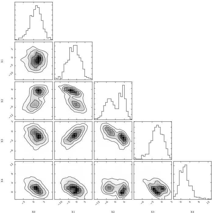
The observations D represented in Fig. 3 are random samples with α = 1 and β = −1. Our goal is to infer the values α and β based on D. We construct the log-likelihood ratio

− 2 log Λ(α, β) = −2 log p(D|α, β)

sup_α,βp(D|α, β) (4.3)

that we calculate via Eqn. 3.6. Following the procedure described in Sec. 3.2, we build a single 2-layer neural network (with 5+2 inputs and one output node) to form the

parame-terized classifier s(x; θ0, θ1) and fix θ1 = (α = 0, β = 0). Since the generative model is not

expensive, the classifier output is calibrated on-the-fly with histograms for every candidate parameter pair (α, β).

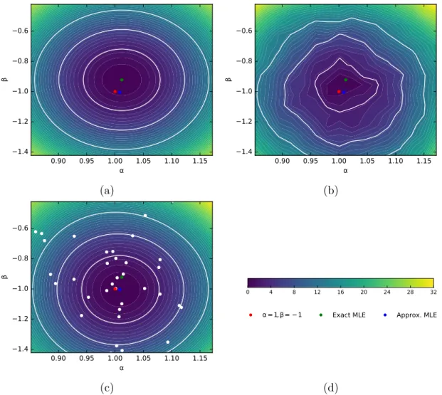
Figure 4a shows the exact log-likelihood ratio for this dataset, which has an exact MLE

at ( ˆα = 1.012, ˆβ = −0.9221). Figure 4b shows the approximate log-likelihood ratio

eval-uated on a coarse grid of parameter values. Some roughness in the contours is observed, which is primarily due to variance introduced in the calibration procedure. In addition

(20)

10 5 0 5 X 1 12 6 0 6 X 2 6 3 0 3 X 3 3 0 3 X0 0 4 8 12 X 4 10 5 0 5 X1 12 6 0 6 X2 6 3 0 3 X3 0 4 8 ₁₂ X4

Figure 3: Scatter plots for the 500 samples in the 5-dimensional data D generated for nominal values (α = 1, β = −1).

(21)

0.90 0.95 1.00 1.05 1.10 1.15 α 1.4 1.2 1.0 0.8 0.6 β (a) 0.90 0.95 1.00 1.05 1.10 1.15 α 1.4 1.2 1.0 0.8 0.6 β (b) 0.90 0.95 1.00 1.05 1.10 1.15 α 1.4 1.2 1.0 0.8 0.6 β (c) 0 4 8 12 16 20 24 28 32

α =1, β= −1 Exact MLE Approx. MLE

(d)

Figure 4: Inference from exact and approximate likelihood ratios. The red dot corresponds to the true values (α = 1, β = −1) used to generate D, the green dot is the MLE from the exact likelihood, while the blue dot is the MLE from the approximate likelihood. 1, 2 and 3-σ contours are shown in white. (4a) The exact −2 log Λ(α, β) for the observed data D. (4b) The approximate −2 log Λ(α, β) evaluated on a coarse 15 × 15 grid. (4c) A Gaussian Process surrogate of −2 log Λ(α, β) ratio estimated from a Bayesian optimization procedure. White dots show the parameter points sampled during the optimization process.

(22)

to the statistical fluctuations due to finite calibration samples, there are also fluctuations introduced from changes in the binning of the calibration histograms as α and β vary. As discussed in Sec. 3.3, a parameterized calibration procedure should ameliorate this issue, but that is left for now as an area for future work. Nevertheless, optimizing the approxi-mate log-likelihood ratio with a Bayesian optimization (Brochu et al., 2010; GPyOpt, 2015) procedure is efficient and effective. After 50 likelihood evaluations, the maximum likelihood

estimate is found at ( ˆα = 1.008, ˆβ = −1.004). While the objective of the Bayesian

opti-mization procedure is to find the maximum likelihood, the posterior mean of the internal Gaussian process, shown in Fig. 4c, is close to the exact log-likelihood ratio illustrated in Fig. 4a. In each case, the true values α = 1 and β = −1 are contained within the 1 − σ likelihood contour.

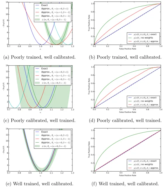
Finally, we evaluate the diagnostics described in Sec. 3.5 for this example. To aid in visualization, we restrict to a 1-dimensional slice of the likelihood along α with β = −1. We consider three situations: i) a poorly trained, but well calibrated classifier; ii) a well trained, but poorly calibrated classifier; and iii) a well trained, and well calibrated classifier. For each case, we employ two diagnostic tests. The first checks for independence of −2 log Λ(θ)

with respect to changes in the reference value θ1 as shown in Eqn. 3.6. The second uses a

classifier to distinguish between samples from p(x|θ0) and samples from p(x|θ1) weighted

according to r(x; θ0, θ1). As discussed for Fig. 4b, statistical fluctuations in the calibration

lead to some noise in the raw approximate likelihood. Thus, we show the posterior mean of a Gaussian processes resulting from Bayesian optimization of the raw approximate likelihood as in Fig. 5c. In addition, the standard deviation of the Gaussian process is shown for one

of the θ1reference points to indicate the size of these statistical fluctuations. It is clear that

in the well calibrated cases that these fluctuations are small, while in the poorly calibrated case these fluctuations are large. Moreover, in Fig. 5a we see that in the poorly trained,

(23)

0.7 0.8 0.9 1.0 1.1 1.2 1.3 α 0 2 4 6 8 10 12 14 − 2l og Λ (θ ) Exact Approx., θ1=(α=0,β=1) Approx., θ1=(α=1,β=−1) Approx., θ1=(α=0,β=−1) ±1σ, θ1=(α=0,β=−1)

(a) Poorly trained, well calibrated.

0.0 0.2 0.4 0.6 0.8 1.0 False Positive Rate

0.0 0.2 0.4 0.6 0.8 1.0

True Positive Rate

p(x|θ1)r(x|θ0,θ1) exact

p(x|θ1) no weights

p(x|θ1)r(x|θ0,θ1) approx.

(b) Poorly trained, well calibrated.

(c) Poorly calibrated, well trained.

0.0 0.2 0.4 0.6 0.8 1.0

True Positive Rate

p(x|θ1) no weights

(d) Poorly calibrated, well trained.

(e) Well trained, well calibrated.

0.0 0.2 0.4 0.6 0.8 1.0

True Positive Rate

p(x|θ1) no weights

(f) Well trained, well calibrated.

Figure 5: Results from the diagnostics described in Sec. 3.5. The rows correspond to the quality of the training and calibration of the classifier. The left plots probe the sensitivity

to θ1, while the right plots show the ROC curve for a calibrator trained to discriminate

(24)

well calibrated case the classifier ˆs(x; θ0, θ1) has a significant dependence on the θ1reference point. In contrast, in Fig. 5c the likelihood curves vary significantly, but this is comparable to the fluctuations expected from the calibration procedure. Finally, Fig. 5e shows that in the well trained, well calibrated case that the likelihood curves are all consistent with the exact likelihood within the estimated uncertainty band of the Gaussian process. The ROC curves tell a similarly revealing story. As expected, the classifier is not able to distinguish

between the distributions when p(x|θ1) is weighted by the exact likelihood ratio. We can

also rule out that this is a deficiency in the classifier because the two distributions are well

separated when no weights are applied to p(x|θ1). In both Fig. 5b and Fig. 5d the ROC

curve correctly diagnoses deficiencies in the approximate likelihood ratio ˆr(ˆs(x; θ0, θ1)).

Finally, Fig. 5f shows that the ROC curve in the well trained, well calibrated case is almost identical with the exact likelihood ratio, confirming the quality of the approximation.

Overall, this example further illustrates and confirms the ability of the proposed method for inference with multiple parameters and multi-dimensional data where reliable

approxi-mations ˆp(x|θ0) and ˆp(x|θ1) are often difficult to construct.

4.3 High energy physics

High energy physics was the original scientific domain that motivated the development of this procedure. In high energy physics, we are often searching for some class of events, generically referred to as signal, in the presence of a separate class of background events. For

each event we measure some quantities x, with corresponding distributions ps(x|ν) for signal

and pb(x|ν) for background, where ν are nuisance parameters describing uncertainties in

the underlying physics prediction or response of the measurement device. The total model is a mixture of the signal and background, and µ is the mixture coefficient associated to

(25)

the signal component, that is

p(D|µ, ν) = Y

x∈D

[µps(x|ν) + (1 − µ)pb(x|ν)] . (4.4)

Accordingly, new particle searches are typically framed as hypothesis tests where the null corresponds to µ = 0, and the generalized likelihood ratio is used as a test statistic.

Nuisance parameters are an after thought in the typical usage of machine learning in high energy physics. The classifiers are typically trained with data generated using a fixed

nominal value of the nuisance parameters ν = ν0. However, as experimentalists we know

that we must account for the systematic uncertainties that correspond to the nuisance

parameters ν. Thus, typically we take the classifier ˆs(x) as fixed and then propagate

uncertainty by estimating ˆps(ˆs(x)|ν) with a parameterized calibration procedure. However,

this classifier is clearly not optimal for ν 6= ν0. In contrast, a parameterized classifier

proposed in this work would yield more accurate estimates of the generalized likelihood ratio.

In addition to robustness to systematic uncertainties incorporated by the nuisance pa-rameters ν, the proposed method can be used to infer papa-rameters of interest. Not only can the mixture coefficient µ be inferred using the decomposition procedure, but also physical parameters like particle masses that change the distribution of x. This formalism represents a significant step forward in the usage of machine learning in high energy physics, where classifiers have always been used between two static classes of events and not parameterized explicitly in terms of the physical quantities we wish to measure.

Another approach for parameter inference with multi-dimensional data specific to high energy physics is the so-called matrix element method, in which one directly computes an approximate likelihood ratio by performing a computationally intensive integral associated to a simplified detector response (Volobouev, 2011). In the approach considered in this

(26)

paper, the detailed detector response is naturally incorporated by the simulator; however, that integral is intractable for the matrix element method. Even with drastic simplifications of the detector response, the matrix element method can take several minutes of CPU time to calculate the likelihood ratio for a single event x. The work here can be seen as aiming at the same conceptual target, but relying on machine learning to overcome the complexity of the detector simulation. It also offers enormous speed increase for evaluating the likelihood at the cost of an initial training stage. In practice, the matrix element method has only been used for searches and measurement of a single physical parameter (sometimes with a single nuisance parameter as in (Aaltonen et al., 2010)).

Contemporary examples where the technique presented here could have major impact include the measurement of coefficients to quantum mechanical operators describing the production and decay of the Higgs boson (Chen et al., 2015) and, if we are so lucky, measurement of the mass of supersymmetric particles in cascade decays (Allanach et al., 2000). Both of these examples involve data sets with many events, each with a feature vector x that has on the order of 10 components, and a parameter vector θ with 2-10 parameters of interest and possibly many more nuisance parameters.

5 Related work

The closest work to the proposed method is due to Neal (2007), who similarly considers the problem of approximating the likelihood function when only a generative model is available. That work sketches a scheme in which one uses a classifier with both x and θ as an input to serve as a dimensionality reduction map. The key distinction comes in the handling of θ. Neal argues that a classifier cannot be used on real data, since we do not know the correct value for θ, and goes on to outline an approach where one uses regression on a

(27)

per-event basis to estimate ˆθ(x) and perform the composition s(x; ˆθ(x)). As pointed out by the author, this can lead to a significant loss of information since a single observation x may carry little information about the true value of θ, though a full data set D may be informative. The work of Neal (2007) correctly identifies this as an approximation of the target likelihood even in the case of a ideal classifier. In contrast, the approach described here does not eliminate the dependence of the classifier on θ. Instead, we embed a parameterized classifier into the likelihood and postpone the evaluation of the classifier to the point of evaluation of the likelihood when θ is explicitly being tested. This avoids

the loss of information that occurs from the regression step ˆθ(x) proposed by Neal (2007)

and leads to Thm. 1, which is an exact result in the case of an ideal classifier. In both cases, the quality of the classifier is factorized from the calibration of its density, which allows for valid inference even if there is a loss of power due to a non ideal classifier.

Also close to our work, Scott and Nowak (2005) and Xin Tong (2013) consider the machine learning problem associated to Neyman-Pearson hypothesis testing. In a simi-lar setup, they consider the situation where one does not have access to the underlying distributions, but only has i.i.d. samples from each hypothesis. This work generalizes that goal from the Neyman-Pearson setting to generalized likelihood ratio tests and em-phasizes the connection with classification. Ihler et al. (2004) take on a different problem (tests of statistical independence) by using machine learning algorithms to find scalar maps from the high-dimensional feature space that achieve the desired statistical goal when the fundamental high-dimensional test is intractable.

More generally, likelihood ratio testing directly relates to the density ratio estimation problem, which consists in estimating the ratio of two densities from finite collections of

observations D0 and D1. Density ratio estimation is connected to many machine learning

(28)

prob-abilistic classification and regression (Vapnik, 1998), outlier detection (Hido et al., 2011), and many others. For learning under covariate shift, Shimodaira (2000) and Sugiyama and

M¨uller (2005) estimate the density ratio r(x; θ0, θ1) from straightforward approximations

ˆ

p(x|θ0) and ˆp(x|θ1) separately obtained using kernel density estimation. Despite its

theo-retical consistency, this approach is known to be ineffective in practice (Sugiyama et al., 2007; Bickel et al., 2009), since it relies on modeling numerator and denominator high-dimensional densities, which is a harder problem than modeling their ratio only. While the proposed method also proceeds in two similar steps, estimating p(s(x)) is much easier than estimating p(x), since s projects x into a one-dimensional space in which only the infor-mative content of r(x) is preserved. Finally, in contrast with the proposed method which decouples reduction from calibration, other approaches proposed within the literature (see Sugiyama et al. (2012); Gretton et al. (2009); Nguyen et al. (2010); Vapnik et al. (2013)

and references therein) provide solutions for estimating r(x; θ0, θ1) directly from x, in one

step. Under some assumptions, the convergence of the obtained estimates is also proven for some of these approaches.

6 Conclusions

In this work, we have outlined an approach to reformulate generalized likelihood ratio tests with a high-dimensional data set in terms of univariate densities of a classifier score. We

have shown that a parameterized family of discriminative classifiers ˆs(x; θ0, θ1) trained and

calibrated with a simulator can be used to approximate the likelihood ratio, even when it is not possible to directly evaluate the likelihood p(x|θ). The proposed method offers an alter-native to Approximate Bayesian Computation for parameter inference in the likelihood-free setting that can also be used in the frequentist formalism without specifying a prior over

(29)

the parameters. In contrast to approaches that learn the posterior conditional on D, our approach can be applied to any observed data D once trained. A strength of this approach is that it separates the quality of the approximation of the target likelihood from the qual-ity of the calibration. The former leverages the continuing advances in supervised learning approaches to classification. The calibration procedure for a particular parameter point is fairly straightforward since it involves estimating a univariate density using a generative model of the data. The difficulty of the calibration stage is performing this calibration continuously in θ. Different strategies to this calibration are anticipated depending on the dimensionality of θ, the complexity of the resulting likelihood function, or the practical issues associated to running the simulator.

Acknowledgments

KC and GL are both supported through NSF ACI-1450310, additionally KC is supported through PHY-1505463 and PHY-1205376. JP was partially supported by the Scientific and Technological Center of Valpara´ıso (CCTVal) under Fondecyt grant BASAL FB0821. KC would like to thank Daniel Whiteson for encouragement and Alex Ihler for challenging dis-cussions that led to a reformulation of the initial idea. KC would also like to thank Shimon Whiteson, Babak Shahbaba for advice in the presentation, Radford Neal for discussion of his earlier work, Yann LeCun, Philip Stark, and Pierre Baldi for their feedback on the

project early in its conception, Bal´azs K´egl for feedback to the draft, and Yuri Shirman for

reassuring cross checks of the Theorem. KC is grateful to UC-Irvine for their hospitality while this research was carried out and the Moore and Sloan foundations for their generous support of the data science environment at NYU.

(30)

References

Aaltonen, T. et al. (2010). Top Quark Mass Measurement in the Lepton + Jets Channel Using a Matrix Element Method and in situ Jet Energy Calibration. Phys.Rev.Lett., 105:252001.

Agostinelli, S. et al. (2003). GEANT4: A Simulation toolkit. Nucl.Instrum.Meth.,

A506:250–303.

Allanach, B., Lester, C., Parker, M. A., and Webber, B. (2000). Measuring sparticle masses in nonuniversal string inspired models at the LHC. JHEP, 0009:004.

Baak, M., Gadatsch, S., Harrington, R., and Verkerke, W. (2015). Interpolation between multi-dimensional histograms using a new non-linear moment morphing method. Nuclear Instruments and Methods in Physics Research Section A: Accelerators, Spectrometers, Detectors and Associated Equipment, 771:39–48.

Baldi, P., Cranmer, K., Faucett, T., Sadowski, P., and Whiteson, D. (2016). Parameterized Machine Learning for High-Energy Physics. arXiv preprint arXiv:1601.07913.

Beaumont, M. A., Zhang, W., and Balding, D. J. (2002). Approximate bayesian computa-tion in populacomputa-tion genetics. Genetics, 162(4):2025–2035.

Bickel, S., Br¨uckner, M., and Scheffer, T. (2009). Discriminative learning under covariate

shift. The Journal of Machine Learning Research, 10:2137–2155.

Brochu, E., Cora, V. M., and De Freitas, N. (2010). A tutorial on bayesian optimization of expensive cost functions, with application to active user modeling and hierarchical reinforcement learning. arXiv preprint arXiv:1012.2599.

(31)

Chen, Y., Di Marco, E., Lykken, J., Spiropulu, M., Vega-Morales, R., et al. (2015). 8D likelihood effective Higgs couplings extraction framework in h → 4`. JHEP, 1501:125. Cowan, G., Cranmer, K., Gross, E., and Vitells, O. (2010). Asymptotic formulae for

likelihood-based tests of new physics. Eur.Phys.J., C71:1554.

Cranmer, K., Lewis, G., Moneta, L., Shibata, A., and Verkerke, W. (2012). HistFactory: A tool for creating statistical models for use with RooFit and RooStats. CERN-OPEN-2012-016.

Friedman, J., Hastie, T., Tibshirani, R., et al. (2000). Additive logistic regression: a statistical view of boosting (with discussion and a rejoinder by the authors). The annals of statistics, 28(2):337–407.

GPyOpt (2015). GPy: A bayesian optimization framework in python. http://github. com/SheffieldML/GPyOpt.

Gretton, A., Smola, A., Huang, J., Schmittfull, M., Borgwardt, K., and Sch¨olkopf, B.

(2009). Covariate shift by kernel mean matching. Dataset shift in machine learning, 3(4):5.

Hido, S., Tsuboi, Y., Kashima, H., Sugiyama, M., and Kanamori, T. (2011). Statisti-cal outlier detection using direct density ratio estimation. Knowledge and information systems, 26(2):309–336.

H¨ormander, L. (1990). The Analysis of Linear Partial Differential Operators I. Springer

Science, Business Media.

Ihler, A., Fisher, J., and Willsky, A. (2004). Nonparametric Hypothesis Tests for Statistical Dependency. IEEE Transactions on Signal Processing, 52(8):2234–2249.

(32)

Lin, Y. (2002). Support vector machines and the bayes rule in classification. Data Mining and Knowledge Discovery, 6(3):259–275.

Louppe, G., Cranmer, K., and Pavez, J. (2016). carl: a likelihood-free inference toolbox. http://dx.doi.org/10.5281/zenodo.47798, https://github.com/diana-hep/carl. Neal, R. M. (2007). Computing likelihood functions for high-energy physics experiments when distributions are defined by simulators with nuisance parameters. In Proceedings of PhyStat2007, CERN-2008-001, pages 111–118.

Nguyen, X., Wainwright, M. J., Jordan, M., et al. (2010). Estimating divergence func-tionals and the likelihood ratio by convex risk minimization. Information Theory, IEEE Transactions on, 56(11):5847–5861.

Pedregosa, F., Varoquaux, G., Gramfort, A., Michel, V., Thirion, B., Grisel, O., Blondel, M., Prettenhofer, P., Weiss, R., Dubourg, V., Vanderplas, J., Passos, A., Cournapeau, D., Brucher, M., Perrot, M., and Duchesnay, E. (2011). Scikit-learn: Machine learning in Python. Journal of Machine Learning Research, 12:2825–2830.

Read, A. (1999). Linear interpolation of histograms. Nuclear Instruments and Methods in Physics Research Section A: Accelerators, Spectrometers, Detectors and Associated Equipment, 425(1):357–360.

Scott, C. and Nowak, R. (2005). A neyman-pearson approach to statistical learning. IEEE Trans. Inform. Theory, 51:3806–3819.

Shimodaira, H. (2000). Improving predictive inference under covariate shift by weighting the log-likelihood function. Journal of statistical planning and inference, 90(2):227–244.

(33)

Sjostrand, T., Mrenna, S., and Skands, P. Z. (2006). PYTHIA 6.4 Physics and Manual. JHEP, 0605:026.

Sugiyama, M. and Kawanabe, M. (2012). Machine learning in non-stationary environments: Introduction to covariate shift adaptation. MIT Press.

Sugiyama, M., Krauledat, M., and M¨uller, K.-R. (2007). Covariate shift adaptation by

importance weighted cross validation. The Journal of Machine Learning Research, 8:985– 1005.

Sugiyama, M. and M¨uller, K.-R. (2005). Input-dependent estimation of generalization error

under covariate shift. Statistics & Decisions, 23(4/2005):249–279.

Sugiyama, M., Suzuki, T., and Kanamori, T. (2012). Density ratio estimation in machine learning. Cambridge University Press.

The ATLAS Collaboration (2012). Observation of a new particle in the search for the Standard Model Higgs boson with the ATLAS detector at the LHC. Phys.Lett., B716:1– 29.

The CMS Collaboration (2012). Observation of a new boson at a mass of 125 GeV with the CMS experiment at the LHC. Phys.Lett., B716:30–61.

Vapnik, V. (1998). Statistical learning theory, volume 1. Wiley New York.

Vapnik, V., Braga, I., and Izmailov, R. (2013). Constructive setting of the density ratio estimation problem and its rigorous solution. arXiv preprint arXiv:1306.0407.

Volobouev, I. (2011). Matrix Element Method in HEP: Transfer Functions, Efficiencies, and Likelihood Normalization. arXiv preprint arXiv:1101.2259.

(34)

Xin Tong (2013). A Plug-in Approach to Neyman-Pearson Classification. Journal of Machine Learning Research, 14:3011–3040.

A

Probabilistic classification for building s

In this appendix, we show for completeness that the probabilistic classification framework yields a reduction s which satisfies conditions of Thm. 1.

Proposition 2. Let X = (X1, ..., Xp) and Y be random input and output variables with

values in X ⊆ Rp and Y = {0, 1} and mixed joint probability density function pX,Y(x, y).

For the squared error loss, the best regression function s : X 7→ [0, 1], or equivalently the best probabilistic classifier, is

s∗(x) = P (Y = 1)pX|Y(x|Y = 1)

P (Y = 0)pX|Y(x|Y = 0) + P (Y = 1)pX|Y(x|Y = 1)

. (A.1)

Proof. For the squared error loss,

s∗(x) = arg min s(x) E Y |X=x{(Y − s(x))2} = arg min s(x) E Y |X=x{Y2} − 2s(x)EY |X=x{Y } + s(x)2 = arg min s(x) −2s(x)EY |X=x{Y } + s(x)2 (A.2)

The last expression is minimized when _ds(x)d _(−2s(x)EY |X=x{Y } + s(x)2) = 0, that is when

−2EY |X=x{Y } + 2s(x) = 0, hence

(35)

For Y = {0, 1},

EY |X=x{Y } = P (Y = 0|X = x) × 0 + P (Y = 1|X = x) × 1

= P (Y = 1)pX|Y(x|Y = 1)

pX(x)

= P (Y = 1)pX|Y(x|Y = 1)

P (Y = 0)pX|Y(x|Y = 0) + P (Y = 1)pX|Y(x|Y = 1)

. (A.4)

For P (Y = 0) = P (Y = 1) =1_/₂_{, the best regression function s}∗ _{simplifies to}

s∗(x) = pX|Y(x|Y = 1)

pX|Y(x|Y = 0) + pX|Y(x|Y = 1)

. (A.5)

If we further assume that samples for Y = 0 (resp. Y = 1) are drawn from some

pa-rameterized distribution with probability density pX(x|θ0) (resp. pX(x|θ1)), then the best

regression function can be rewritten as

s∗(x) = pX(x|θ1)

pX(x|θ0) + pX(x|θ1)

. (A.6)

In particular, this regression function satisfies conditions of Thm. 1 since s∗(x) = m(r(x; θ0, θ1)),

for m(r(x)) = (1 + r(x))−1, is monotonic with r(x; θ0, θ1).

Proposition 2 holds for the squared error loss, but it can be similarly shown that classi-fiers minimizing the exponential loss, the binomial log-likelihood (or cross-entropy) or the squared hinge loss are also monotonic with the density ratio (Friedman et al., 2000; Lin, 2002). However, a classifier with discrete outputs and minimizing the zero-one loss does not satisfy conditions of the theorem.