HAL Id: dumas-01634570
https://dumas.ccsd.cnrs.fr/dumas-01634570
Submitted on 14 Nov 2017
HAL is a multi-disciplinary open access archive for the deposit and dissemination of sci-entific research documents, whether they are pub-lished or not. The documents may come from teaching and research institutions in France or abroad, or from public or private research centers.
L’archive ouverte pluridisciplinaire HAL, est destinée au dépôt et à la diffusion de documents scientifiques de niveau recherche, publiés ou non, émanant des établissements d’enseignement et de recherche français ou étrangers, des laboratoires publics ou privés.
Investigating the trophic ecology of five species of
Gadiformes in the Celtic Sea combining stable isotopes
and gut contents
Louise Day
To cite this version:
Louise Day. Investigating the trophic ecology of five species of Gadiformes in the Celtic Sea combining stable isotopes and gut contents . Agronomy. 2017. �dumas-01634570�
Investigating the trophic ecology of five species of
Gadiformes in the Celtic Sea combining stable
isotopes and gut contents
Par : Louise DAY
Soutenu à Rennes le 13 septembre 2017
Devant le jury composé de :
Président : Didier Gascuel, Agrocampus Ouest Maître de stage : Dorothée Kopp, IFREMER Lorient Enseignant référent : Didier Gascuel, Agrocampus Ouest
Autres membres du jury
Jean-Marc Roussel, INRA Rennes
Hervé Le Bris, Agrocampus Ouest (maître de stage)
Les analyses et les conclusions de ce travail d'étudiant n'engagent que la responsabilité de son auteur et non celle d’AGROCAMPUS OUEST AGROCAMPUS OUEST CFR Angers CFR Rennes Année universitaire : 2016 - 2017 Spécialité : Agronomie
Spécialisation (et option éventuelle) :
Sciences Halieutiques et Aquacoles – Ressources et Ecosystèmes Aquatiques
Mémoire de Fin d'Études
d’Ingénieur de l’Institut Supérieur des Sciences agronomiques, agroalimentaires, horticoles et du paysage
de Master de l’Institut Supérieur des Sciences agronomiques, agroalimentaires, horticoles et du paysage
d'un autre établissement (étudiant arrivé en M2)
Ce document est soumis aux conditions d’utilisation
«Paternité-Pas d'Utilisation Commerciale-Pas de Modification 4.0 France» disponible en ligne http://creativecommons.org/licenses/by-nc-nd/4.0/deed.fr
Remerciements
Je remercie mes trois encadrants de stage Marianne Robert, Dorothée Kopp et Hervé Le Bris pour leurs précieux conseils et leur présence pendant ces six mois. Je remercie à nouveau Hervé pour l’attention sans faille qu’il m’a portée tout au long de ce stage et avec qui j’ai beaucoup appris, et notamment à identifier des proies à moitié digérées. Je remercie l’équipe « Ecologie Halieutique » pour leur accueil chaleureux et cette ambiance agréable qui en émane. Merci à Catherine, Sophie, Etienne, Olivier, Didier, Jérôme, Elodie, Marie, Amélie, Marine, Hubert, Pierre-Yves, Maud, Morgane, Shani, Déborah et Max, mon super camarade de bureau.
Cette étude n’aurait pas été possible sans le travail d’échantillonnage et de laboratoire réalisé au préalable Je remercie donc Marianne et Dorothée ainsi que toutes les personnes qui ont participé à l’échantillonnage des espèces étudiées à bord du Thalassa sur les campagnes EVHOE 2014 et 2015. Je remercie également Margaux Denamiel pour son travail sur les contenus stomacaux et sur la préparation des échantillons isotopiques.
Résumé étendu en français
Etude compare de l’écologie trophique de cinq espèces de Gadiformes en
mer Celtique à partir de deux approches : les isotopes stables et les
contenus digestifs
Contexte
Il est bien connu que dans un écosystème marin, les espèces présentes interagissent de plusieurs manières. On compte parmi ces multiples interactions celles d’ordre trophique : prédation inter et intra espèce ou encore compétition pour une même ressource alimentaire. De plus, pratiquement toutes les pêcheries sont multi spécifiques de par le fait que les engins utilisés peuvent difficilement ne cibler qu’une seule espèce. Partant de ces deux constats, la communauté scientifique recommande d’opter pour une vision écosystémique des systèmes marins et de baser les outils de gestion sur cette approche. Cette dernière reconnait les interactions trophiques et techniques entre les espèces commerciales ou non, et permettant ainsi une meilleure gestion des ressources marines. La mise en place d’une telle gestion nécessite de collecter des informations locales et récentes sur la nature des interactions entre espèces et notamment : qui mange qui ou quoi ? Ces données servent alors à alimenter des modèles écosystémiques qui à leur tour permettent de diagnostiquer l’état d’un système et de prédire ses réactions face à des changements de gestion ou globaux. L’étude en amont de l’écologie trophique des espèces est donc essentielle à la robustesse de ces modèles.
L’écologie trophique est une science ancienne qui s’intéresse donc aux niches trophiques des espèces, aux facteurs qui les influencent (avec entre autre l’ontogénie et l’habitat) et aux interactions entre ces espèces. Historiquement, ces études étaient menées via l’analyse de contenus stomacaux et l’observation des comportements alimentaires. Aujourd’hui, les scientifiques ont également recours à l’analyse des isotopes stables, un outil qui permet de déterminer la position trophique d’un individu et les sources consommées par ce dernier.
La mer Celtique est située entre l’Irlande, la Bretagne et le Pays de Galles. C’est une zone d’importance majeure pour les pêcheries européennes. Le présent travail vise à étudier l’écologie trophique de cinq espèces de gadiformes (la morue, l’églefin, le merlan, le merlu et le merlan bleu), toutes exploitées en mer Celtique par des pêcheries mixtes.
Objectifs
L’objectif de cette étude est donc de déterminer les différences et les similarités dans la niche trophique de ces cinq espèces, qui partagent des caractères physiques du fait de leur appartenance à un même groupe taxonomique. On cherche alors à étudier la compétition entre ces espèces, mais aussi des potentielles différences ontogénétiques (via deux classes de taille) et spatiales (via deux zones – une profonde et une moins profonde) dans les niches trophiques
de ces espèces. Cette étude s’appuie sur une double approche méthodologique : analyse des contenus digestifs et analyse des signatures isotopiques.
Matériel et Méthodes
Pour réaliser cette analyse, deux types de données ont été utilisées : des contenus digestifs et des signatures isotopiques pour chacune des espèces dans les deux zones et pour les deux classes de taille. Tout d’abord, la composition des régimes alimentaires a été décrite pour chaque espèce, chaque classe de taille et chaque zone. En parallèle, les effets de l’espèce, de la taille et de la zone sur les signatures isotopiques ont été analysés à l’aide de régressions linéaires. Ensuite, les niches trophiques ont été décrites à l’aide de leur largeur estimée via la richesse taxonomique pour les contenus digestifs et via l’aire du nuage isotopique. Cette aire, représentant 40% de la variance des données, a été estimée avec une approche bayésienne afin de mesurer l’incertitude associée. Ensuite, les recouvrements de niches ont été abordés à partir d’un indice mesurant le taux de similarité entre les contenus digestifs et le pourcentage de recoupement des aires de niches isotopiques. Enfin, des modèles de mélange bayésiens ont été construits afin d’estimer, à partir des signatures isotopiques du réseau trophique, les contributions relatives des différents groupes préalablement identifiés.
Résultats et discussion
Cette étude a confirmé le caractère généraliste de ces cinq espèces avec une importante diversité de proies à l’échelle des populations. Ces espèces se situent globalement en haut du réseau trophique de mer Celtique. Cependant, leurs niches trophiques présentent chacune des particularités les séparant les unes des autres. L‘églefin consomme exclusivement des proies benthiques (échinodermes et mollusques). La morue se nourrit pour une grande partie sur des décapodes (crabes, anomoures ou langoustines) nécrophages et présente ainsi un très haut niveau trophique. La part de poissons dans son alimentation reste faible et contredit les études précédentes. Cependant, les contenus digestifs sont le reflet d’un aperçu instantané et peuvent biaiser notre vision. L’églefin et la morue sont les espèces avec la diversité de proies la plus élevée, cependant, leur niche isotopique ne reflète pas cette étendue. Le merlan possède une large niche trophique s’alimentant sur les voies pélagique et benthique, de crustacés et poissons faisant de lui un top-prédateur du système. Le merlu est une espèce presque exclusivement piscivore et présente un niveau trophique inférieur aux trois autres prédateurs. Son alimentation est en partie pélagique, ce qui impliquerait une alternance entre chasse dans la colonne d’eau et repos sur le fond. Enfin, le merlan bleu est un zooplanctonophage et constitue une proie pour la morue, le merlu et le merlan.
Des shifts ontogénétiques ont été mis en évidence pour le merlu et dans une moindre mesure, pour le merlan et l’églefin. Le merlu passe d’un régime composé de crustacés et de poissons à un régime largement dominé par les poissons, ceci est confirmé par les signatures isotopiques. Les signatures isotopiques de l’églefin montrent un changement brutal entre les deux classes de taille, cependant les contenus digestifs révèlent une relative constance du régime. La morue ne semble pas changer radicalement d’alimentation entre le stade juvénile et le stade adulte,
contrairement à des études plus anciennes ou dans des écosystèmes voisins. Ces changements de régime et de niveau trophique observés ici peuvent être reliés à l’arrivée de la maturité et donc à une demande énergétique supplémentaire, le tout étant permis par la modification des caractères biologiques tels que la largeur de la bouche ou la vitesse de nage.
Les contenus digestifs révèlent une plus grande diversité de proies dans la zone peu profonde, confirmé par une niche isotopique plus large à l’échelle de la communauté. Cependant, les ressources présentes, et donc disponibles dans ces zones, ne sont pas connues et ne permettent pas de conclure quant à une telle différence. De plus, il semblerait que le couplage entre les compartiments pélagique et benthique soit plus faible en zone profonde à cause d’une stratification plus forte des masses d’eau. Toutefois les contenus digestifs ne nous permettent pas de confirmer ce résultat, puisque ce dernier dépend également d’une correction appliquée aux données isotopiques.
Conclusion
Finalement, cette étude montre que ces cinq espèces très proches dans la classification possèdent des comportements et préférences alimentaires assez différents. Dans l’établissement de modèles, ces spécificités sont à intégrer, de même que le shift ontogénétique du merlu. Des indices tendent à montrer une différence de structure trophique entre les deux zones. Cependant, une enquête plus approfondie des ressources disponibles ou en analysant un plus grand nombre d’espèces serait appropriée. Une des perspectives majeures de ce travail est l’étude des variations saisonnières et annuelles des niches trophiques pour avoir une image plus complète et plus proche de la réalité.
Table of contents
1 INTRODUCTION ... 1
1.1 Towards an ecosystem-based fisheries management approach ... 1
1.2 Influence of biotic and abiotic environment on the trophic niche ... 2
1.3 Studying feeding ecology ... 2
1.4 Study case: 5 species of Gadiformes in the Celtic Sea ... 4
2 MATERIEL AND METHODS ... 7
2.1 Data collection ... 7
2.1.1 Sampling design: definition of size classes and areas ... 7
2.1.2 Gut contents ... 8
2.1.3 Stable isotopes... 9
2.2 Data analyses ... 10
2.2.1 Gut contents analysis ... 10
2.2.2 Stable isotopes analysis ... 11
3 RESULTS ... 14
3.1 Gut contents analyses ... 14
3.1.1 Diet description ... 14
3.1.2 Taxonomic prey richness and feeding strategy ... 15
3.1.3 Diet overlap ... 18
3.2 Stable isotopes analyses ... 19
3.2.1 Predators stable isotope signatures ... 19
3.2.2 Trophic level ... 21
3.2.3 Isotopic niche breadth ... 22
3.2.4 Isotopic niche overlaps... 23
3.2.5 Predators’ location in the food web ... 23
3.2.6 Estimated proportions of assimilated prey ... 25
4 DISCUSSION ... 26
4.1 Usefulness of improving our knowledge on the enrichment factor ... 27
4.2 Limits of the baseline correction of isotopic values ... 27
4.3 Species trophic niche in the Celtic Sea ... 28
4.4 Ontogenetic shift in diet and trophic niche ... 30
4.5 Spatial effect on trophic niche ... 32
5 CONCLUSION AND PERSPECTIVES ... 33
REFERENCES ... 36
List of figures
Figure 1: Catches of the five species studied in the Celtic Sea from 1980 to 2014 (Statland database http://www.ices.dk/marine-data/dataset-collections/Pages/Fish-catch-and-stock-assessment.aspx compiled by ICES). ... 4 Figure 2 : Map of EVHOE stations where Gadiformes were sampled during the campaigns 2014 and 2015 for the EATME program. ... 8 Figure 3: Photographs taken during gut contents identification a: pelagic Copepoda (scale = 1.6 mm), b: blue whiting Micromesistius poutassou otoliths (1.5 mm), c: bivalve Cardiidae (0.8 mm), d: cephalopod beak (2 mm), e: shrimp Crangon allmanni telson (3 mm), f: shrimp Spirontocaris liljeborgii (2 mm). ... 9
Figure 4: Relative abundance of prey phyla in the digestive content of each predator categories for both zones. ... 14 Figure 5: Taxonomic richness (a) comparison between raw taxonomic richness and estimated taxonomic richness from the rarefaction curve with n = 15 (lowest common denominator) for each predator category (b) comparison between zones; triangles represent raw counts of richness and error bars are the estimated richness. ... 16 Figure 6: Tokeshi graphical representation of population diversity (Shannon index) against mean individual diversity (a) explanatory diagram for interpretation of feeding strategy according to Tokeshi (1991) and (b) diagram for the 5 species, 2 size classes (indicated by the numbers 1 and 2 linked by arrows) in both zones. The arrows represent ontogenetic shifts. .. 17 Figure 7: Two-dimensional ordination from non-metric multidimensional scaling on predator categories (coloured labels) and prey groups (grey polygons) from %FO tab - ben: benthic invertebrates, dem: demersal fish, pel_c: pelagic crustaceans and pel_f: pelagic fish. Numbers (1 and 2) indicate position of the two size classes for a predator category (stress = 0.13). ... 18 Figure 8: Sample size-corrected standard ellipse (SEAc) from δ15N and δ13C values for each prey category in both zones. The crosses and points represent the raw isotopic data and lines the SEAc. ... 21 Figure 9: Trophic level calculated from Post’s equation (2002) for each predator categories in both zones. Boxplots represent the median and quantiles; red point with the value is the mean. ... 22 Figure 10: Posterior Bayesian estimates of the standard ellipse area (SEAb in grey) and sample size-corrected standard ellipse area (SEAc red crosses) for each prey category in both zones. ... 22 Figure 11: Isospace of the trophic web in zone 1 displaying species average stable isotopes values (colored dots) and the sources average stable isotopes values (colored crosses). ... 24 Figure 12 : Isospace of the trophic web in zone 2 displaying species average stable isotopes values (colored dots) and the sources average stable isotopes values (colored crosses). ... 24
List of tables
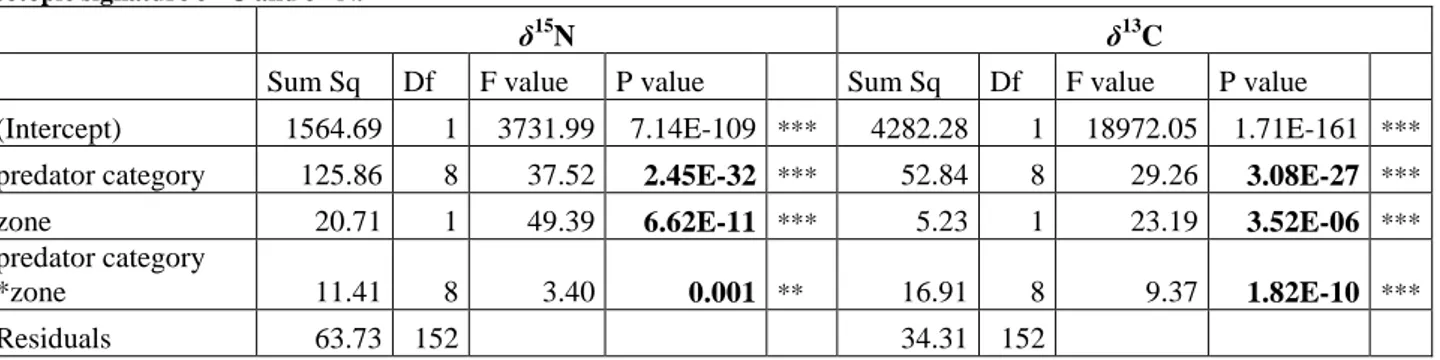
Table 1: Size classes of the five species based on size measures taken during EVHOE campaigns from 1998 to 2013. ... 7 Table 2: Characteristics on feeding strategy: taxonomic richness, estimated taxonomic richness (for n=15), number of different taxa per fish and number of preys per fish for each predator category. ... 16 Table 3: Schoener’s overlap index between predator categories in both zones. The shaded cells indicate a Schoener index superior to 50%. ... 19 Table 4: Results of ANOVAs procedures prior to MN and MC selecting the variables to
explain the variability of isotopic signature δ13C and δ15N. ... 20 Table 5: Isotopic characteristics: δ15N and δ13C composition, standard ellipse area corrected (SEAc). ... 20 Table 6: Estimated proportions of assimilated prey clusters (in %) in the diet of the predators in both zones with: mode (1st column), mean (2nd column) and standard error (3rd column) of each prey proportion distribution. A selection of the most probable clusters was made prior of running SIAR in order to limited the number of sources. ... 25
List of Appendices
Appendix I: Sample design for guts and stable isotopes samples. Appendix II: Composition of the functional groups of prey.
Appendix III: Linear regression of isotopic values of Pecten maximus in function of depth Appendix IV: Occurrence (%) of prey groups for each predator category and for both zones. Appendix V: Relative abundance (%) of prey groups for each predator category and for both zones.
Appendix VI: Rarefaction curves for the five Gadiformes for each size class and each zone (the orange line represents n = 15 sampling units, the lowest common denominator).
Appendix VII: Relative abundance (%N) of prey position in the water column (benthic, demersal, pelagic or non-identified) in the digestive content of each predator categories for both zones.
Appendix VIII: Residuals’ analyses for Gaussian linear model on δ13C and δ15N values. Appendix IX: Summary of the MN and MC (where the null hypothesis corresponds to the
nullity of the difference between the first coefficient for a given factor and the other coefficients)
Appendix X-A: Overlaps between ellipses of the 9 predator categories in the zone 1. Appendix X-B: Overlaps between ellipses of the 9 predator categories in the zone 2.
1
1 I
NTRODUCTION
1.1 Towards an ecosystem-based fisheries management approach
Fisheries management science and stock evaluations have been realized using a single-stock approach for decades. Exploited Europeans species are generally evaluated independently of other populations and proposals of quotas by the International Council for the Exploration of the Sea (ICES) are stock-specific. Yet, virtually all fisheries are multi-specific as fishing gears cannot target a single species. In order to reach the goal of sustainability in fisheries, the scientific community recommend to switch to an ecosystem-based fishery management (Botsford et al., 1997; Pikitch et al., 2004). Ecosystem-based management is a holistic approach which acknowledges that exploited species interact with other species and the environment.
Technically, this approach requires the development of multi-species and ecosystemic models. Several scientific teams had developed such models. For example, Multi-Species Virtual Population Analysis MSVPA (Helgason and Gislason, 1979; Pope, 1979) or the more recent Stochastic Multi-Species model SMS (Lewy and Vinther, 2004) are operational models in terms of management. On the other hand, models such as Ecopath-With-Ecosim Ewe (Christensen and Pauly, 1992; Christensen and Walters, 2004; Polovina, 1984), Object-oriented Simulator of Marine ecOSystem Exploitation OSMOSE (Shin and Cury, 2004) allow a better understanding of the functioning and the trophic interactions within a given ecosystem. They also are comprehensive tools to predict the future trophic functioning under different fishing scenarios. All these models acknowledge that species interact, notably predation and competition interactions. Then, models rely on trophic data and information in order to estimate predation between the species or trophic compartments. Fisheries management can be greatly improved by relying on ecosystemic approach as trophic interactions are crucial in understanding resource dynamics. Pope (1991) explained that in the North Sea, the multi-species model revealed a fresh point of view of the trophic functioning and in terms of fishing impacts compared to single-species models. Indeed, the multi-species model resulted in a decreased of the overall yield when reducing the fishing mortality because of an increase of the predation. Additionally, ecosystemic models allow taking into consideration technical interactions between fleets: a given species could be captured by several fishing gears and so several fleets.
To get robust estimations, models should be based on local trophic data (Heymans et al., 2016). As this resource is scare, they often use data from similar close supposed ecosystem. Therefore, one major drawback of these models is the need of accurate and local diet information (Moullec et al., 2017). Indeed, fish diet may vary according to numerous factors, including depth (Kopp et al., 2015) and local prey availability (Pinnegar et al., 2003). Thus, studying and understanding the trophic ecology of the all the species within a given ecosystem, with a particular attention for commercial species, is essential in the implementation of an ecosystem approach to fisheries.
2
1.2 Influence of biotic and abiotic environment on the trophic niche
The concept of ecological niche has several definitions and modifications through time as some ecologists defined it as a reference to an environment and some others to species (Pulliam, 2000). This concept of niche is fundamental as it is the base of how species use resources (Bearhop et al., 2004). Hutchinson (1957) described the ecological niche as an ‘n dimensional space’ which axes represent environmental variables. Among these variables, the food resources constitute the trophic niche.
Trophic niche could vary according to several factors, such as ontogeny (especially the development stage or size), habitat, sex, season, geographical position, depth, local prey availability and, more generally, on various abiotic and biotic environmental factors.
The size is one of the most important attribute for an organism in terms of ecology as it determines the needs in energy (Werner and Gilliam, 1984). Ontogenetic shifts influence the biologic interactions with others species and so predation interactions. As fish grow, their morphometric attributes and physical abilities evolve such as increase in mouth dimension (Karpouzi and Stergiou, 2003; Keast and Webb, 1966) or improvement in swimming performance (Gibb et al., 2006). These ontogenetic changes allow fish to ingest a larger range of prey items larger or faster prey for example (Karpouzi and Stergiou, 2003; Pinnegar et al., 2003). Hence, diet composition and trophic position within the ecosystem of a given species is likely to evolve with ontogenesis. In an ecosystem modelling approach, such information on species could lead to make pertinent choices. For example, in Ewe models, it is possible to separate size classes in different trophic compartments (i.e. to create “stanzas”).
Among fish, change of diet with the size is very common and is often correlated with a change of habitats (Werner and Gilliam, 1984). Indeed, habitats could have different prey offers according to environmental variables (depth, salinity, sediment type, etc.). In aquatic systems, depth is an important factor in regulation of the benthic-pelagic coupling. Depth is a regulator of the degree of interactions between the water column and the water close to the bottom (Schindler and Scheuerell, 2002). Indeed, with depth occurs the phenomenon of stratification of the water mass stratification. Stratification results from differences in the density of the water column caused mainly by temperature (and so solar radiation) and differential in salinity (Baustian et al., 2014). Benthic-pelagic coupling is the interactions between the two environments, mainly driven by organism movements, biogeochemical cycling and trophic interactions (Baustian et al., 2014). For example, Lassalle et al. (2011) concluded from a Ewe model set in the Bay of Biscay that demersal fish species, and in particular suprabenthivorous species, are an important link between the pelagic and the benthic layers as they feed on benthic organisms and are preyed by large pelagic consumers. In the Channel Sea, the benthic-pelagic coupling was investigated as a function of depth and it appeared that the coupling is stronger in shallow waters and weakens with depth increasing (Giraldo et al., 2017; Kopp et al., 2015). For example, with increasing depth, demersal species have a more and more benthic diet whereas pelagic predators concentrate their foraging effort on pelagic prey (Giraldo et al., 2017).
1.3 Studying feeding ecology
Feeding ecology of marine organisms is a key component to understand their roles and importance in the food web. Trophic studies allow answering to important ecological issues such as predation, position within the food web or competition.
3 Historically, investigating the trophic niche of marine species relied on gut contents analysis GCA (Hyslop, 1980). This approach is essential as it allows fine resolution in taxonomic prey identification. However, GCA has several limits. First, the prey identification is extremely time-consuming and requires good knowledge on consumed species. Then, it provides only a snapshot of the diet, showing the last ingested prey. Moreover, stomach content analysis is biased toward prey items which are not readily digested (Jackson et al., 1987).
Stable isotopes analysis SIA is a useful and contemporary tool for studying the trophic ecology and niche in estuarine and marine systems (Peterson and Fry, 1987; Layman et al., 2012; Fry 2007). Isotopes are chemical elements which occupy the same place in the periodic table as they have the same proton number but differ in neutron number. Isotopes can be natural or artificial and stable or unstable. In ecological and trophic studies, the most commonly used naturally occurring stable isotope ratios are carbon (13C:12C expressed as δ13C in ‰ units) and nitrogen (15
N:14N expressed as δ15N). SIA are based on two useful properties of isotopes: isotope fractionation and natural variations of their abundance. DeNiro and Epstein (1978) stated: “You are what you eat… plus a few per mil”. Fractionation represents the fact that δ15N and δ13C values are transformed from dietary sources to consumers. Consumer’s composition is generally higher than its prey; this is referred to enrichment (Phillips et al., 2014). This is due to phenomena of isotopes’ discrimination according to their atomic mass during assimilation and excretion. Indeed, early lab studied demonstrated that lighter isotopes are preferentially used by metabolism, resulting in enrichment in heavier isotopes (DeNiro and Epstein, 1978). The trophic enrichment factor (TEF or Δ) depends on multiple factors such as the given element, tissue and organism (Phillips, 2012). So far, it has been accepted by the scientific community that the average values for Δδ13C and Δδ15N range between 0 and 1‰ and between 3 and 4‰, respectively(DeNiro and Epstein, 1978; Minagawa and Wada, 1984; Peterson and Fry, 1987). Consequently δ15N measurements serve as indicators of a consumer's trophic level as a result of bioaccumulation of heavy isotopes
15
N (Post, 2002). Oppositely, carbon isotope ratios are rather stable through trophic levels and enable to trace back the origin of the carbon sources in a given environment (DeNiro and Epstein, 1978). For example, (France, 1995) showed that benthic sources were 13C enriched compared to pelagic algae. As δ13C present also natural gradient, they can be used to trace habitats and organisms migrations. Comparing δ13C latitude variations and δ13C measurement from fur seals’ whiskers, Kernaléguen et al. (2012) demonstrated a spatial foraging gradient between species and sex.
SIA is increasingly used thanks to the numerous benefits it provides. The development of effective technologic tool (mass spectrometry) allows us to obtain data with automated process and easy quantification of the proportions from each prey eaten by a predator. Stable isotopes are data with a integration of several weeks of the assimilated diet and time-integration depends on the tissue sampled (Phillips et al., 2014).
Newsome et al. (2007) provided a review on the use of stable isotopes in order to investigating the trophic niches. They discussed the concept of isotopic niche as “an area (in with isotopic values as coordinates”. The isotopic niche is often represented as bivariate plots with δ13C values on the x-axis, δ15N values on the y-axis and variance estimates.
However, SIA should be interpreted with caution as two predators with the same isotopic compositions have not necessarily the same prey and stable isotopes cannot allow identification of specific prey. Hence, guts and isotopic approaches are complementary in the study of diet and trophic niche as their association allows a better understanding of the
4 feeding ecology and processes. Many studies today combine the two methods, on various species and places as seals in Artic (Dehn et al., 2007), snow crab Chionoecetes opilio (Divine et al., 2017) or elasmobranchs in the Gulf of Mexico (Churchill et al., 2015).
1.4 Study case: 5 species of Gadiformes in the Celtic Sea
The Celtic Sea (Divisions VIIe-k according to the classification of ICES) is a major fishing area in Europe, mainly exploited by Ireland, France, the United Kingdom, Spain and Belgium. This is a large continental shelf with a sandy bottom. Most of the area is shallower than 200 m and is bounded to the west by a steep and rocky slope. In order to better understand the trophic functioning of the Celtic sea and develop a multi-species model for fisheries management, the EATME program was started in 2014 by IFREMER with the mission of collecting data on local fish diet. Isotopic data and stomach contents of 10 commercial species were sampled. Among those species, five belong to the Gadiformes family: the Atlantic cod Gadus morhua (Linnaeus 1758), the haddock Melanogrammus aeglefinus (Linnaeus 1758), the whiting Merlangius merlangus (Linnaeus 1758), the European hake Merluccius merluccius (Linnaeus 1758) and the blue whiting Micromesistius poutassou (Risso 1827).
These five species present an important commercial interest. As an order of magnitude, in 2009 around 30,000 t were caught. The demersal fisheries catches were estimated to 120,000 tons in 2008 in both the Celtic Sea and the Bay of Biscay (Guénette and Gascuel, 2012). About three quarters of the catches can be attribute to the Celtic Sea only (Moullec, 2015). With a rough estimation, we estimated the demersal catches in the Celtic Sea around 90,000 t in 2009. Hence, the 5 species represented about one third of the demersal catches in tons in 2009. The other two third were composed by large crustaceans, monkfish and species of flatfish (Guénette and Gascuel, 2012).
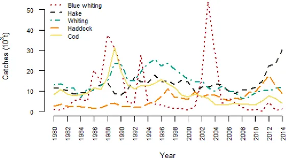
Figure 1: Catches of the five species studied in the Celtic Sea from 1980 to 2014 (Statland database http://www.ices.dk/marine-data/dataset-collections/Pages/Fish-catch-and-stock-assessment.aspx compiled by ICES). Figure 1 shows the temporal evolution of the catches of the five species. G. morhua and M. merlangus have experienced high capture level in tons in the 1980’s and the 1990’s, with between 2 and 3 times today’s level (Figure 1). In contrast, haddock’s catches are increasing since the 1980’s. Hake’s catches raise recently due to an amelioration of the stock status with
5 a decrease of fishing mortality and an increase of the spawning biomass (ICES, 2016a). Blue whiting’s catches are highly variable due to the variations of the recruitment1
(ICES, 2016b). Fisheries in the Celtic Sea are highly mixed and are targeting a range of species with different gears. Among them, the mixed gadoid fishery (cod, haddock and whiting) using beam trawls is responsible of more than 75% of the landings for these species in the ICES areas 7.f and 7.g (ICES, 2016c). Hake is captured by gillnetters, beam trawlers and pelagic trawlers (ICES, 2016a). Blue whiting is caught by large pelagic trawlers (ICES, 2016b) and is the by-catch of demersal fisheries.
These five species of gadiformes present morphological similarities as they come from a common ancestor. They have an elongated body with three dorsal fins and one or two anal fins (Muus et al., 1998). Among these species M. merluccius belongs to the family Merluciidae and the four others to the Gadidae family. Members of Gadidae are demersal or benthopelagic species inhabiting circumpolar and temperate waters. They usually have a chin barbel. Merluciidae species do not have barbel but a large and terminal mouth with pointed teeth in most species. They are known as top predators present on continental shelf and upper slope (Froese and Pauly, 2017).
The European hake is a demersal species widely distributed in the European waters at depths from 30 to 1,000 meters (Belloc, 1929). Its mouth is filled with sharp
teeth. Source: European Commission - FISHERIES
The Atlantic cod is also a demersal species widely distributed in the Atlantic Ocean (off the European and American coasts). It is an omnivorous predator feeding on
fish, molluscs, crustaceans, annelids (Muus et al., 1998). Source: European Commission - FISHERIES The haddock is a demersal species present in European
and American waters, presents at depths from 10 to 200 meters. It has a downward directed, protrusible mouth which enables it to feed on benthic prey (Muus et al.,
1998). Source: fiheries.no the official Norwegian site
The whiting is a voracious predator present along the European coasts. Juveniles have a small barbell and adults
don’t (Muus et al., 1998). Source: Iceland Quality Seafood The blue whiting is a bathy-pelagic fish widely distributed
throughout the North Atlantic at depths from 100 to 400 meters, near the continental slope (Muus et al., 1998;
Sorbe, 1980). Source: fiheries.no the official Norwegian site It is therefore of interest to study the diversity of the trophic niches and the feeding strategies within one taxonomic group presenting common biological traits and being often fished simultaneously in the same areas. It is essential to gain insight on their trophic interactions notably the competition and the predation existing between these species in order to understand their population co-dynamics. To this end, emphasis will be laid on the comparison between species and size classes as we explained that size is a key factor in determining of diet. Additionally, as depth could create disparities in trophic niche, we will explore the effects of two areas in the Celtic Sea on the feeding ecology of these species.
6 Global problematic
Are there differences in trophic ecology of these five commercial gadiformes with taking into account two areas (proxy of a depth gradient) and two size classes (proxy of ontogeny) in the highly exploited Celtic Sea?
This work will seek to answer to two aims:
a. Investigate the trophic structure between the two zones for the 5 species and potential ontogenetic shifts in trophic niche and diet
b. Compare the two methodologic approaches: are they complementary or do they suggest two different views of the trophic functioning?
Hypotheses
(1) Interspecific variability
Diets observed in this study will be compared to the scientific literature on one side and to the diet matrix of a Ewe model in the Celtic Sea recently published. Moullec et al. (2017) built an Ecopath models in order to understand trophic functioning of the Celtic Sea and the Bay of Biscay. They used a diet matrix as an input of the model and they obtained trophic level among outputs for the 2013 model. The diet matrix was based on a review of literature on diet in similar ecosystems. Thus, we assumed from these data that G. morhua and M. merluccius are top predators in this ecosystem, feeding mainly on small demersal fish, shrimps, sardine and carnivorous invertebrates for cod and boarfish, horse mackerel, mackerel, pouts, shrimps and zooplankton for hake. M. aeglefinus feeds mainly on surface suspension and deposit feeders, demersal fish and sub-surface deposit feeders invertebrates. M. merlangus is considered as an omnivorous species feeding on a numerous number of preys including many fish species, pelagic and benthic and macrozooplankton. Finally, M. poutassou is a planktivorous species preying on macro/mesozooplankton and shrimps.
(2) Size influence on diet and trophic niche
Larger individuals consume larger bodied prey although they keep consuming smaller ones (Pinnegar et al., 2003). Hence, we hypothesize that larger predators have wider trophic niches than small ones. Moreover, we hypothesize that larger predators feed on a higher proportion of fish as demonstrated for M. merluccius in the bay of Biscay and the Celtic Sea by Mahe et al. (2007) and for G. morhua in the Celtic Sea by Du Buit (1995); which could lead to higher trophic level for larger predators.
(3) Local feeding strategies
We hypothesize that the weakening of the coupling between the pelagic and the benthic compartments with a depth-gradient (Giraldo et al., 2017; Kopp et al., 2015) accentuates with a deeper depth-gradient. Benthic sources increases in demersal feeders’ diet with increasing depth (i.e. from zone 1 to 2) whereas pelagic feeders feed on more important part of pelagic sources.
7
2 M
ATERIEL AND METHODS
2.1 Data collection
2.1.1 Sampling design: definition of size classes and areas
Fish were collected in November 2014 and 2015 during EVHOE campaigns (Evaluation des ressources halieutiques de l'ouest européen) on board R/V “Thalassa” in the Celtic Sea. Fishing operations were realized using a GOV (Grande Ouverture Verticale) 36/47 demersal trawl, towed for 30 min at a speed of approximately 3.5 knots. It has an opening of 20 m horizontally and 4 m vertically. The net is fitted with a 20 mm cod end liner stretched mesh. As part of the IBTS (International Bottom Trawl Survey) protocol, all fishing operations were carried out during daytime.
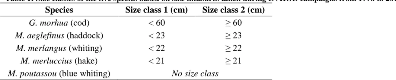
To evaluate the potential ontogenetic shifts within trophic niches, size classes were established. To optimize the sampling effort, size classes were chosen before collecting data according to the main modes observed in the size distribution of each species obtained during previous EVHOE campaigns 1998-2013. For M. aeglefinus, M. merlangus, M. merluccius and G. morhua, 2 modes were distinguishable, hence two size classes were considered. For M. poutassou, only one mode could be observed on the histogram, hence all individuals were considered from the same size class. The limits between the two size classes for each species are summarized in Table 1.
Table 1: Size classes of the five species based on size measures taken during EVHOE campaigns from 1998 to 2013.
Species Size class 1 (cm) Size class 2 (cm)
G. morhua (cod) < 60 ≥ 60
M. aeglefinus (haddock) < 23 ≥ 23
M. merlangus (whiting) < 22 ≥ 22
M. merluccius (hake) < 21 ≥ 21
M. poutassou (blue whiting) No size class
The size classes chosen were consistent with a well-known meaningful biological parameter: the length at maturity. G. morhua matures around 50-70 cm in the Celtic Sea (Brander, 2005). M. aeglefinus reaches maturity between 20 and 25 cm in the North Sea in 2005 (Wright et al., 2011). M. merlangus matures around 19-22 cm in the Irish Sea (Gerritsen et al., 2003). A study in the Bay of Biscay and the Galician coast showed that length at maturity for M. merluccius is between 40 and 50 cm (Domínguez-Petit et al., 2008).
8 Figure 2 : Map of EVHOE stations where Gadiformes were sampled during the campaigns 2014 and 2015 for the EATME program.
In order to explore the potential effect of the geographical location on trophic niches and diet preferences, samples we collected in two zones. EVHOE survey design is based on strata based on depth and location (south, central, north part of the Celtic Sea and Bay of Biscay). To optimize the sampling effort, EVHOE strata were grouped by performing clustering analysis on annual abundances of species sampled during EVHOE since 1998. Two zones were identified, gathering different EVHOE stratas, based on homogeneous specific composition (Figure 2): a shallow inshore one from 71 m to 119 m deep in the central Celtic Sea (zone 1) and a deeper offshore one from 121 m to 158 m (zone 2) on the continental shelf. The sampling design is summarized in Appendix I.
2.1.2 Gut contents Sample preparation
On-board, all fishes were measured. Guts of the five species of Gadiformes were dissected and frozen for subsequent analyses back in the laboratory.
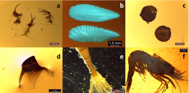
At the laboratory, guts were thawed and then emptied to retrieve prey that were in the stomach and the intestine. Gut contents were placed in a Petri dish and prey were identified at the most precise taxonomic level using a binocular stereoscopic magnifier Leica outfitted with a Leica IC80 HD camera (Figure 3). A total of 593 guts were analysed. Most of the guts were full for cod and haddock with vacuity rates between 0 and 12%. Blue whiting had an intermediate vacuity rate with 18 and 13% in zone 1 and 2 respectively. Hake and whiting had high vacuity rates between 13 and 54% (Appendix I). Only individuals with non-empty guts have been considered for further analysis.
The largest part of the laboratory work has been made by Margaux Denamiel and I realised the 5 % left during 3 weeks of this internship in Agrocampus laboratory with the help of Hervé Le Bris.
9 Figure 3: Photographs taken during gut contents identification a: pelagic Copepoda (scale = 1.6 mm), b: blue whiting
Micromesistius poutassou otoliths (1.5 mm), c: bivalve Cardiidae (0.8 mm), d: cephalopod beak (2 mm), e: shrimp Crangon allmanni telson (3 mm), f: shrimp Spirontocaris liljeborgii (2 mm).
Prey grouping
Prey were grouped to ease interpretation of the results. The grouping was chosen according to 3 factors: the taxonomy (crustaceans, echinoderms…), the position in the water column (pelagic, demersal, and benthic) and the trophic guild (carnivore, omnivore, deposit feeder, suspension feeder…). Hence, from 156 different taxa identified we end up with 37 functional groups. The composition of each prey group is detailed in Appendix II. Main contributions to predators’ diet were highlight using the frequency of occurrence and relative abundance (Appendices IV and V). Occurrence and abundance were chosen over bulk methods as they are more robust (Baker et al., 2014). Bulk methods appeared to have a high level of uncertainty because digested material cannot easily be separated.
2.1.3 Stable isotopes Samples preparation
On-board, a sample of white dorsal muscle was dissected (Pinnegar and Polunin, 1999) and frozen on a subset of individuals. At the laboratory, samples were oven dried 60°C during 48 h and ground into a homogeneous powder using a mixer mill. Samples were sent to the Stable Isotopes in Nature Laboratory (University of New Brunswick, Canada) where they were analysed using a Carlo Erba NC2500 Elemental Analyzer. Stable isotopes values were converted into ratio (δ notation):
𝛿𝑋 = [ 𝑅𝑠𝑎𝑚𝑝𝑙𝑒
𝑅𝑠𝑡𝑎𝑛𝑑𝑎𝑟𝑑 − 1] × 10
3 (𝑖𝑛 ‰)
where R is 13C/12C or 15N/14N. The international standard references are Pee Dee Belemite carbonate for δ13C and atmospheric nitrogen for δ15N. Normalization of δ13C ratios for species with a C:N higher than 3.5 (the value above which lipid normalization is recommended ; Post et al., 2007) was performed according to the following equation (Post et al., 2007):
𝛿13𝐶
𝑛𝑜𝑟𝑚𝑎𝑙𝑖𝑧𝑒𝑑 = 𝛿13𝐶𝑢𝑛𝑡𝑟𝑒𝑎𝑡𝑒𝑑− 3.32 + 0.99 𝐶: 𝑁
a
b
c
10
2.2 Data analyses
2.2.1 Gut contents analysis Taxonomic richness
Precautions should be taken when comparing taxonomic richness from unbalanced sampling as predator categories containing different numbers of samples (Chao et al., 2014; Colwell et al., 2012). The taxonomic richness increases with the number of units sampled in a non-linear way. As our sampling was unbalanced (in zone 1, 41 guts were dissected for small cod and 15 for larger ones), rarefaction curves were estimated for each predator category in order to gain robustness in comparing taxonomic richness using the R package “INEXT” (Hsieh et al., 2016). Curves were constructed with unconditioned variance and predators were compared using an estimation of taxonomic richness for n = 15 (the lowest number of guts for a predator category – except small M. merlangus in zone 2).
Niche breadth
Piélou index, also known as the normalized Shannon’s index, was used to evaluate the trophic niche breadth. This index is equal to 0 when the considered predator is fully specialist and prey only upon one prey type and it is equal to 1 when the predator is generalist and consumes all possible prey types equally:
𝑃𝑖é𝑙𝑜𝑢𝑖 = − 1 ln 𝑁∑ 𝑝𝑖,𝑘 𝑁 𝑘=1 ln 𝑝𝑖,𝑘
where N is the total number of prey taxon groups and pi,k is the relative abundance of prey
taxon k in the diet of predator species i. Feeding strategy
Tokeshi (Tokeshi, 1991) is a graphical method to evaluate the feeding strategy of a predator by using the mean individual feeding diversity (DI) plotted against the population feeding diversity (DP) defined by the following formulas:
𝐷𝐼 = −1
𝑁∑ 𝑝𝑖,𝑘ln 𝑝𝑖,𝑘
𝑖,𝑘
𝐷𝑃 = − ∑ 𝑝𝑖ln 𝑝𝑖 𝑖
where N is the total number of predators, pi,k the proportion of prey item i in the kth predator
and pi the proportion of prey i in the entire population.
Links between prey community and predators
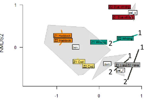
To visualise differences in community structure and predator categories/prey groups relationships between the two areas, an unconstrained ordination method: the non-metric multi-dimensional scaling (MDS) was carried out (Kruskal, 1964). A selection of prey groups was preliminarily made to exclude scarce groups which could lead to difficulties in MDS interpretation (Manté et al., 2003). Prey groups were thus selected for these MDS analyses when the frequency of occurrence was superior to 5% for at least one predator category. In order to perform this analysis, we formed a matrix of dissimilarities using the Bray-Curtis
11 dissimilarity calculation. Non-metric MDS is a rank-based approach i.e. it is based on rank orders instead of original distance. The quality of the representation was validated with a stress under 0.3. Stress relates pairwise distances between objects in the reduced ordination space to their dissimilarities in the “real world”, the complete multidimensional space. nMDS is an iterative process which optimize the stress by minimizing it.
Diet overlaps
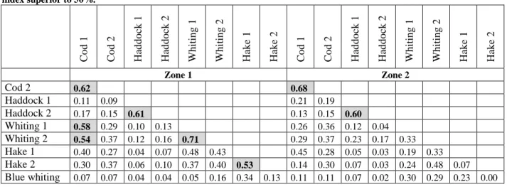
The Renkonen similarity index (Renkonen, 1938) also known as the Schoener overlap index (Schoener, 1970) was used to access niche overlaps between predators by constructing a similarity matrix. The similarity between the predators i and j was given by:
𝑠𝑖,𝑗= ∑ min (𝑝𝑖,𝑘, 𝑝𝑖,𝑘)
𝑁
𝑘=1
where pi,k and pj,k are relative abundances of prey species k for predator i and predator j,
respectively. The index ranges from 0 (no feeding overlap), to 1 (same distribution of prey). 2.2.2 Stable isotopes analysis
Baseline correction
Isotopic values of the baseline of a trophic web might vary along environmental gradients such as the inshore-offshore gradient or depth gradient (Chouvelon et al., 2012; Nerot et al., 2012; Schaal et al., 2016). In the study of higher consumers and comparison between different areas, there is a need to spatially adjust their isotopic values. Indeed, without baseline correction, it is impossible to distinguish variations in the isotopes ratios due to spatial variations of the base of the food chain or due to changes in the food web structure. Hence, an artificial rescaling allowed us to compare trophic structure between areas. Ideally, this correction should be done using the primary producers of the ecosystem as the base, but they have highly variable isotopes ratios (Jennings and Warr, 2003). Thus, Cabana and Rasmussen (1996) suggested to use primary consumers as bivalves as they have more stable signatures and are supposed to mainly feed on primary producers. Suspension feeding bivalves, Pecten maximus were chosen as the trophic baseline for this study.
Hence, raw isotopic data for both nitrogen and carbon were corrected with baseline isotopic values. We decided to correct the raw data according to the depth of the collection as it expressed spatial heterogeneity. First, a linear Gaussian regression was realised to investigate the relationship between the isotopic values of P. maximus and the depth (Appendix III):
𝛿𝑋𝑃.𝑚𝑎𝑥𝑖𝑚𝑢𝑠(𝑑𝑒𝑝𝑡ℎ, 𝑖) = 𝛼 ∗ 𝑑𝑒𝑝𝑡ℎ + 𝛽 + 𝜀𝑖 ~ 𝑁(0, 𝜎²)
After checking graphically the residuals (normality and homoscedasticity) in order to validate the model’s hypothesis, we used the coefficients of the regression in order to correct the raw data of each consumer sample by subtracting the predicted baseline at the sampling location (considering only depth) and by adding the mean of the baseline isotopic values for the given element in the whole zone:
𝛿𝑋𝑐𝑜𝑟𝑟𝑒𝑐𝑡𝑒𝑑 = 𝛿𝑋𝑢𝑛𝑐𝑜𝑟𝑟𝑒𝑐𝑡𝑒𝑑 − [𝛼 ∗ 𝑑𝑒𝑝𝑡ℎ𝛿𝑋+ 𝛽] + 𝑚𝑒𝑎𝑛(𝛿𝑋𝑃.𝑚𝑎𝑥𝑖𝑚𝑢𝑠 𝑖𝑛 𝐶𝑒𝑙𝑡𝑖𝑐 𝑆𝑒𝑎)
12 Trophic level (TL)
Trophic level was estimated using Post equation (Post, 2002):
𝑇𝐿𝑖 = 𝛿15𝑁𝑖 − 𝛿15𝑁𝑏𝑎𝑠𝑒
3.4 + 2
where δ15Ni is the corrected δ15Nvalue for the individual i and δ15Nbase is the mean of all P.
maximus δ15N values. TL for a predator category was then calculated by averaging the
individual TLs.
Stable isotopes compositions
The effects of the categorical variables: predator category (9 levels, combination of species and size classes), zone (2 levels) and their two-way interactions on isotopic compositions (δ13C and then δ15Nratios) were assessed through Linear Model with an identity link. A preliminary variable selection was performed, using an ANOVA procedure based on Fisher’s tests on δ13C values and then on δ15Nvalues:
(MN) δ15Np,z,i = μ + αp + βz + γp,z + εi ~ N(0,σ²)
(MC) δ13Cp,z,i = μ’ + α’p + β’z + γ’p,z + εi ~ N(0,σ’²)
where i is the individual, p the predator category and z the zone. Models’ hypotheses, normality and variance homogeneity of the residuals, were validated graphically (Appendix VIII). Tukey post hoc tests were performed to evaluate potential shifts between size classes. Isotopic niche
Isotopic niche is defined by Newsome et al. (2007) as an area in the isotopic space where each axe is an element with isotopic values coordinates (δX). To visualize isotopic niches, sample size-corrected standard ellipse area (SEAc) were plotted on bi-plots δ15N/δ13C (Jackson et al., 2011). These ellipses represent the trophic niche of a group by integrating 40% of the sample variance. To avoid a problem of underestimation of the SEA when the sample size is inferior to 30, a corrective factor is applied as following:
𝑆𝐸𝐴𝑐 = 𝑆𝐸𝐴 × (𝑛 − 1)(𝑛 − 2)−1 (𝑖𝑛 ‰2).
The correction approaches 1 when n tends to infinity, which is a desired property here.
For the purpose of comparing isotopic niches between species and size classes, a Bayesian approach was set up to estimate the posterior distribution of the standard ellipse area (SEAb) and then uncertainty was incorporated to SEAc. This method is based on Markok-Chain Monte Carlo (MCMC) draws in the posterior distribution combining the priors and the likelihoods with the followings parameters: 20000 iterations, a discard of the 1000 first values, a run with 2 chains and a thin posterior of 10; and the following priors: an Inverse Wishart prior on the covariance matrix (2 0
0 2) and a vague normal prior on the means (103). The likelihood is a multivariate normal distribution: 𝑌𝑖 ~ 𝑀𝑉𝑁([µ𝑥, µ𝑦], 𝛴), with µx and µy
the means and Σ, the covariance matrix. This procedure was realised using R package ‘SIBER’ (Jackson et al., 2011).
13 Isotopic overlaps
Niches overlaps were estimated and expressed as the percentage of the ellipse area (SEAc) of the niche 1 overlapped by the niche 2 using the R package ‘SIAR’ (Parnell et al., 2010). Mixing model and assimilated prey proportions estimation
Mixing models allow estimating relative contributions of each prey or group of prey from isotopic signatures of the prey (the sources) and the predator (the consumer) and the TEF between the consumer and its sources. However, the sources of uncertainty are numerous with this type of analysis: uncertainty on the data, on the TEF, on the concentration of carbon and nitrogen within an individual, etc. (Phillips et al., 2014). Hence, a Bayesian approach is well suited to deal with the different layers of uncertainty (Parnell et al., 2010) as this approach allows estimation of probability distribution of multiple source contributions to a mixture. When the isotopic signatures of different sources are too close i.e. sources overlap in the isotopic space, mixing model can encounter difficulties in estimating their relative contributions (Phillips et al., 2005).
The EATME program sampled other species than the five gadiformes analysed in this study: many fish species, some large crustaceans and some other invertebrates. In order to reduce the number of potential sources in the mixing model, clustering was performed on each zone community using a Hierarchical ascendant clustering (HAC). The result gives a simplified picture of the species community within each zone. Additionally, it eases the comparison between areas and creates distinct sources for the mixing model. Euclidean distances and Ward method (which minimising the total within-cluster variance) were used. The number of clusters was chosen according to inertia criterion and also to ecological interpretation.
Using clusters established beforehand as sources and predator category as consumer, Bayesian mixing models SIAR (Parnell et al., 2010) were built for each predator categories. Sources’ contributions were not estimated for haddock as we considered that available prey from EVHOE did not reflect its diet. Moreover, the same decision was made for small hake in zone 2 as applying a positive enrichment on carbon led to no potential sources (Figure 12). TEFs were chosen as the more realistic choice according to the suggestions made by Hussey et al., (2014) and Zanden and Rasmussen (2001). TEFs are decreasing as the trophic level increase (Hussey et al., 2014) and Zanden and Rasmussen (2001) gave an order of magnitude for marine fractionation factors. Hence, TEFs between resources and the consumers were chosen at 0.5 ± 1 for δ13C, 3 ± 1 for δ15N of primary consumers clusters and 2 ± 1 for δ15N of other clusters.
In order to reduce the number of possible sources, prey clusters were selected prior to each mixing models according to the predator considered. The selection was made according to biological consideration (for example G. morhua does not feed on pelagic primary consumer) and mixing model constraints (consumer ratio is supposed to be surrounded by the sources adjusted by TEFs). All mixing models were conducted using the R package ‘SIAR’ (Parnell et al., 2010) with no a priori on contributions, 500000 iterations, a burning of 50000 and a thinby of 15.
All analyses were conducted using the software R (R Core Team, 2015) and significant threshold was taken at p ≤ 0.05.
14
3 R
ESULTS
3.1 Gut contents analyses
Among the 1349 prey found in the 466 non-empty guts dissected, 156 different taxa were identified. The digestive state of prey influenced the final taxonomic level identified. Approximately 50% of the prey were identified at a family level and 35% at a species level.
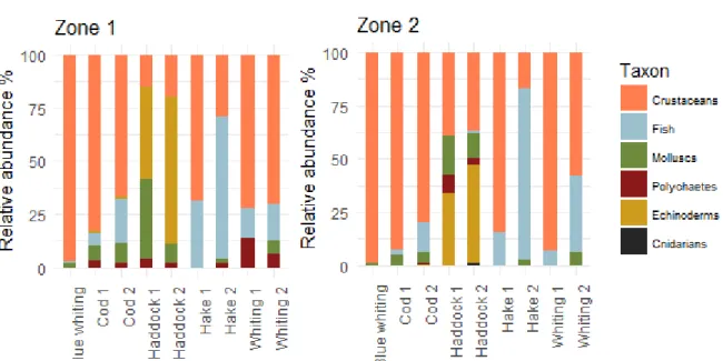
3.1.1 Diet description
Figure 4: Relative abundance of prey phyla in the digestive content of each predator categories for both zones. Different feeding preferences between the five species were identified (Figure 4). G. morhua mainly fed on benthic crustaceans (brachyurans, anomurans and carideans) and to a lesser extent on fish and molluscs (Figure 4, Appendices IV and V). Cod was the only species feeding on Norway lobster Nephrops norvegicus, especially second size class. Large individuals had a larger proportion of fish (Trisopterus esmarkii, Callionymus lyra, Gobiidae and other Gadiformes) than smaller ones in their diet in both zones. Anomurans (Galathea sp. and Munida sp.) had higher occurrences and relative abundances in the diet in zone 2 than in zone 1 with Munida rugosa an important prey in occurrence and abundance. Cod foraged on carnivore and deposit feeder polychaetes in zone 1.
M. aeglefinus largely fed on benthic prey. It was also the only species feeding on echinoderms, particularly sea urchins (Echinocyamus pusillus) in zone 1 and ophiuroids in zone 2 (Figure 4, Appendices IV and V). Large and small individuals had similar diet, with a sentitive larger proportion of molluscs for large haddock than for small one. Haddock also consumed molluscs (as deposit feeder bivalves, essentially Abra spp.), crustaceans (mainly amphipods in zone 2) and to a lesser extend polychaetes with high occurrence frequencies in zone 1 with 40.5% of the small haddock’s guts containing “benthic polychaetes” (Appendix IV). It can be noted that the proportion of echinoderms and molluscs decreased from zone 1 to 2 in favour of crustaceans (Figure 4).
15 M. merlangus had a diversified diet, feeding both on pelagic and benthic prey, both on fish and crustaceans (Figure 4). In zone 1, it mainly fed on crustaceans and especially carideans as Crangon allmanni, amphipods and mysids (Appendices IV and V). A minor part of its diet was composed by fish and polychaetes, such as Lagis koreni. There were few differences between size classes, except that large whiting included cephalopods like Rossia macrosoma or Illex coindetii in their diet. In zone 2, whiting did not consume polychaetes. An increase of the part of the fish in the diet was observed from small to large individuals, with a particular affinity for gadiforms (Micromesistius poutassou, Trachurus trachurus or Trisopterus esmarkii).
M.merluccius was the most piscivorous species. It fed on fish and crustaceans (Figure 4). There was a shift between small and large hakes regarding fish proportion on their diets. Fish represented 66% and 80% of the large hake diet respectively in zone 1 and 2 against 31% and 15% for small hake (Appendix V). Fish prey of large hake was more diversified in zone 1 (pelagic perciforms, gadiforms and clupeiforms) whereas it fed mainly on pelagic gadiforms in zone 2 (Appendices IV and V). Small hake fed mainly on crustaceans as pelagic and benthic carideans (Pasiphaea sivado and Crangon allmanni) in zone 1 and eumalacostraca and pelagic amphipods (Hyperiidea) in zone 2.
M. poutassou fed on pelagic crustaceans. No differences are observed in the relative proportion of prey type between the two areas however, its main prey were pelagic carideans (Pasiphaea sivado) and amphipods (Hyperiidea) in zone 1 and copepods in zone 2 (Figure 4, Appendices IV and V).
Finally, as a large part of the prey items was identified at an imprecise taxonomic level (as order or class), it was not possible to conclude about the proportions of pelagic and benthic prey in the predators’ diet (Appendix VII).
3.1.2 Taxonomic prey richness and feeding strategy
Rarefaction curves showed that the sampling of all predator categories didn’t reach an asymptote (Appendix VI). To access the absolute prey diversity, sampling should be greater. However, using rarefaction curves, it was possible to compare relative taxonomic richness of prey between predator categories.
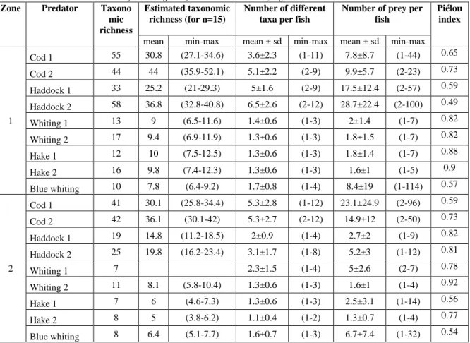
Taxonomic richness was the highest for cod and haddock with estimated richness (for n = 15) between 14.8 and 36.8 taxa respectively whereas other predators’ estimations were between 5 and 10 taxa (Figure 5a, Table 2). These species had also the highest number of different taxa per fish and number of prey per fish, meaning that they had numerous and diverse prey in their guts. Piélou’s index was 0.49 and 0.59 for both size classes of haddock in zone 1 (Table 2). Thus, despite a high taxonomic richness reflecting an opportunist feeding strategy, haddock in zone 1 had preference for some prey items (as E. pusillus). Whiting and hake had close feeding strategies. They had a low number of prey per fish (means between 1.6 and 2.5 preys per individuals) as well as a low diversity of prey (means between 1.1 and 2.3 different taxa per individuals; Table 2). They didn’t show a marked preference for a prey type as they had high Piélou’s index values (except for hake 1 in zone 2: its index is low because of a large part of its diet in the “Eumalacostraca” prey category). Finally, blue whiting had a great number of prey per individual with a mean of 8.4 preys in zone 1 and 6.7 in zone 2 and a low diversity of taxa. Its Piélou’s index was relatively low which confirmed a strong preference for some prey items (Table 2).
16 Figure 5: Taxonomic richness (a) comparison between raw taxonomic richness and estimated taxonomic richness from the rarefaction curve with n = 15 (lowest common denominator) for each predator category (b) comparison between zones; triangles represent raw counts of richness and error bars are the estimated richness.
The global taxonomic richness appeared to be higher in zone 1 since 133 taxa were identified in this zone compared to 83 in zone 2. It was particularly marked for both class sizes of haddock (Figure 5 b) with estimated taxonomic richness of 25.2 and 36.8 for small and large fish in zone 1 and 14.8 and 19.8 in zone 2 respectively (Table 2). However, this pattern was not confirmed at an individual scale as there was no clear difference between zones regarding the mean number of different taxa per fish (Table 2).
Table 2: Characteristics on feeding strategy: taxonomic richness, estimated taxonomic richness (for n=15), number of different taxa per fish and number of preys per fish for each predator category.
Taxonomic richness was not estimated for Whiting 1 in zone 2 as there were only 3 guts dissected. Zone Predator Taxono
mic richness
Estimated taxonomic richness (for n=15)
Number of different taxa per fish
Number of prey per fish
Piélou index
mean min-max mean ± sd min-max mean ± sd min-max
1 Cod 1 55 30.8 (27.1-34.6) 3.6±2.3 (1-11) 7.8±8.7 (1-44) 0.65 Cod 2 44 44 (35.9-52.1) 5.1±2.2 (2-9) 9.9±5.7 (2-23) 0.73 Haddock 1 33 25.2 (21-29.3) 5±1.6 (2-9) 17.5±12.4 (2-57) 0.59 Haddock 2 58 36.8 (32.8-40.8) 6.5±2.6 (2-12) 28.7±22.4 (2-100) 0.49 Whiting 1 13 9 (6.5-11.6) 1.4±0.6 (1-3) 2±1.4 (1-7) 0.82 Whiting 2 17 9.4 (6.9-11.9) 1.3±0.6 (1-3) 1.8±1.5 (1-7) 0.82 Hake 1 12 10 (7.5-12.5) 1.3±0.6 (1-3) 1.8±1.4 (1-7) 0.88 Hake 2 16 9.8 (7.4-12.3) 1.3±0.6 (1-3) 1.6±1 (1-5) 0.9 Blue whiting 10 7.8 (6.4-9.2) 1.7±0.8 (1-4) 8.4±19 (1-114) 0.57 2 Cod 1 41 30.1 (25.8-34.4) 5.3±2.8 (1-12) 23.1±24.9 (2-96) 0.59 Cod 2 42 36.1 (30.1-42) 5.3±2.7 (2-12) 14.9±12 (2-50) 0.73 Haddock 1 19 14.8 (11.2-18.5) 2±0.9 (1-4) 2.7±2 (1-9) 0.82 Haddock 2 25 19.8 (16.2-23.4) 3.1±1.7 (1-8) 5.2±3 (1-12) 0.81 Whiting 1 7 2.3±1.5 (1-4) 5±2.6 (2-7) 0.78 Whiting 2 11 8.1 (5.8-10.4) 1.3±0.6 (1-3) 1.6±1 (1-4) 0.92 Hake 1 7 6 (4.6-7.3) 1.3±0.6 (1-3) 2.5±3.1 (1-14) 0.56 Hake 2 8 5 (3.8-6.2) 1.1±0.4 (1-2) 1.3±0.7 (1-4) 0.77 Blue whiting 8 6.4 (5.1-7.7) 1.6±0.7 (1-3) 6.7±7.4 (1-32) 0.54
a
b
17 Estimated taxonomic richness showed a slightly different pattern compared to the raw taxonomic richness (Figure 5 a). Estimated prey diversity was systematically higher for large cod and haddock in both zones and seemed to be constant for the other categories within each zone.
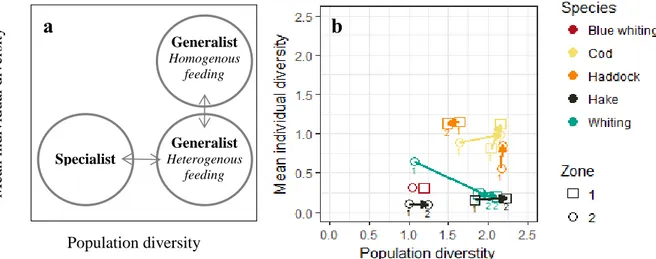
Tokeshi graphical representation summaries differences in the feeding strategies of the 9 predator categories in both zones (Figure 6). As shown in Figure 6-a, the higher the population diversity gets, the more generalist the species is. Generalist species with a lower mean individual diversity are heterogeneous feeding species. Indeed, they have a low diversity taken one by one but the whole population has a high diversity Shannon index.
Figure 6: Tokeshi graphical representation of population diversity (Shannon index) against mean individual diversity (a) explanatory diagram for interpretation of feeding strategy according to Tokeshi (1991) and (b) diagram for the 5 species, 2 size classes (indicated by the numbers 1 and 2 linked by arrows) in both zones. The arrows represent ontogenetic shifts.
Thus, the predators studied presented a generalist feeding behaviour (Figure 6-b). Hake, whiting and blue whiting showed a more heterogeneous feeding strategy than haddock and cod an individual scale. The long arrow linking small and large whitings in zone 2 should be analysed with caution as the small category contained 3 guts. Finally, hake seemed more specialist in zone 2 and haddock adopted a more heterogeneous feeding behaviour in zone 2 compared to zone 1. For other species, no clear difference can be noted between zones.
Generalist Homogenous feeding Generalist Heterogenous feeding Specialist Population diversity Me an ind ivi dua l di ver si ty