A Prior Study of Split Compilation and Approximate Floating-Point Computations

HAL Id: dumas-00636813

https://dumas.ccsd.cnrs.fr/dumas-00636813

Submitted on 28 Oct 2011

HAL is a multi-disciplinary open access

archive for the deposit and dissemination of sci-entific research documents, whether they are pub-lished or not. The documents may come from teaching and research institutions in France or

L’archive ouverte pluridisciplinaire HAL, est destinée au dépôt et à la diffusion de documents scientifiques de niveau recherche, publiés ou non, émanant des établissements d’enseignement et de recherche français ou étrangers, des laboratoires

A Prior Study of Split Compilation and Approximate

Floating-Point Computations

Takanoki Taguchi

To cite this version:

Takanoki Taguchi. A Prior Study of Split Compilation and Approximate Floating-Point Computa-tions. Hardware Architecture [cs.AR]. 2011. �dumas-00636813�

A Prior Study of Split Compilation and Approximate

Floating-Point Computations

Takanori TAGUCHI

Superviser : Erven ROHOU, INRIA - ALF

Master 2 Research, University of Rennes 1

June 2, 2011

Contents

I

Bibliographic Study

3

4 Conclusion : Bibliographic Study 15

II

Internship Report

17

5 Overview 17

6 Related Work 19

6.1 Function Approximation . . . 19 6.2 Speculative Execution . . . 20 6.3 Differences Between Previous Studies and Our Study . . . 24

7 Our Study 24

7.1 Concept of Dynamic Linked Pseudo Math Library . . . 24

7.2 Main Thread . . . 26

7.3 Helper Thread . . . 27

7.3.1 Masking Method and Error Computation . . . 27

7.3.2 History Table . . . 29

7.3.3 Markov Prediction . . . 30

7.4 Shared Data Block and Ownership . . . 31

8 Experiments 35 8.1 Experimental Setup . . . 35

8.2 Results . . . 35

8.3 Evaluation and Further work . . . 36

Abstruct

From a future perspective of heterogeneous multicore processors, we studied several optimization processes specified for floating-point numbers in this internship. To adjust this new generation processors, we believe split compilation has an important role to receive the maximum benefits from these processors. A purpose of our internship is to know a potential of tradeoff between accuracy and speedup of floating-point computa-tions as a prior-study to promote the notion of split compilation. In many case, we can more successfully optimize a target program if we are able to timely apply appropriate optimizations in dynamic. However an online compiler cannot always apply aggressive optimizations because of its constraints like memory resources or compilation time, and the online compiler has to respect these constraints. To overcome these constraints, the split compilation can combine statically analyzed information and dynamic timely information. For this reason, in the bibliographic part, we mainly studied the several compilation method and floating-point numbers to smoothly move to our internship.

Part I

Bibliographic Study

1

Introduction

On a development process of embedded applications, developers cannot avoid con-straints of specific restrictions of each platform on which the application will be executed. Then, reducing these burdens from development process is required in terms of produc-tivity and distributability.

For the technological and economical reasons, nowadays, performance improvements due to increasing of clock frequency will not be expected anymore. Instead, it is expected that applications will be executed in parallel on multicore processors including a case it might be heterogeneous[2, 3, 19]. Although we need a shift to parallel heterogeneous multicore execution, most of legacy code, which has still kept important places, have been written as a sequential execution program. Therefore even if many cores are on a system, it is hard to improve the performance without modifying these legacy codes for parallel execution. And to do so, one must rewrite a large number of lines of legacy code manually. That process is time consuming and it may occur that one modify it unsuitably to original one. In that case, the program behaves incorrectly and it cause a huge loss, since legacy codes have important roles over the world.

For these reasons, the methods which separate the concerns of applications and that of hardware are required. Firstly, the idea of Just-In-Time(JIT) compilation was proposed

and it is widely spread notion at present. But there exist several problems such that JIT compiler cannot apply aggressive and well analyzed optimizations. Because embedded systems cannot have enough resources and during compilation time applications must pause ; it is equal to user waiting time. Hence reducing startup delay and execution on a limited resource are key points for JIT compilation. Then Split Compilation, the subject of my internship, was proposed [3] and it is expected to solve these problems.

The notion of split compilation separates a optimization process to two parts, and as-signs one part to offline compiler (statical compiler) and the other one to online compiler (dynamic compiler, JIT compiler). Compared to split compilation, traditional compila-tion styles entirely attribute one optimizing process either to offline compiler or online compiler. And the split compilation realizes a good performance over several (heteroge-neous) hardware platforms [19, 20].

Additionally, we mention the floating-point issues. Floating-point numbers are used over many domains especially in scientific computations, because of its rich representabil-ity. In fact almost every hardware platform can treat floating numbers. However it is important to understand its implications, because the mechanism is complicated and, for that reason, floating-point number might cause unexpected results [7, 16, 21]. But we need to manage it correctly. Because most programming languages do not give us alternatives, even if floating-point is not the best representation for given application. In this paper, I show how floating-point is complicated and how one should take care not to cause the issues.

The remainder of the paper is organized as follows: In Section 2, we introduce the main notion of compilation and some practical examples of split compilation. In Section 3, we describe the issues concerned with floating-point. Lastly, in Section 4, we conclude our bibliographic work and indicate the direction of the internship.

2

Compilation

In this section, we introduce the main styles of compilation : Static compilation (offline compilation) and Just-In-Time compilation (online compilation, dynamic com-pilation), and we mention their principal optimization phases. After referring to some strong points and weak points of each compilation style, we introduce the notion of Split compilation and explain the reason why we stress the split compilation with some practical examples.

2.1

Static Compilation

A static compiler compiles source code into native code compatible with a partic-ular hardware platform. And all compilation process is done before applications are distributed and executed by users. Because of this compilation style static compilers cannot get run-time information at all, therefore static compilers must take into account

all of the executable paths to optimize source codes. Sometimes static compiler require much resource and compilation time. By using much resource, however, a static compiler can powerfully optimize a source program with precise analysis. This is a advantage of static compilers and many optimization methods are proposed [1].

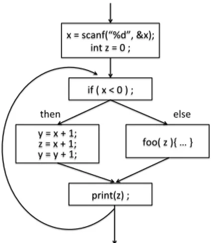
For example, by exploring Control Flow Graph (CFG), static compiler can detect the redundancy of source code and remove it. Especially, if there exist some redundancy in the loop, it may greatly improve its executing time. Because generally 80% of total execution time are spent in 20% part of the code (80/20 rule), and in most case loop executions are included in that part. We show a very simple example like Figure 1. And Figure 2 expresses the Control Flow Graph of the code. By analyzing this CFG, statical compiler can replace z = x + 1 by z = y and this replacement reduces execution cost. Likewise, static compiler can optimize the whole source program. In addition, if x never has positive value during the execution time, we can prune the else part of CFG. It may significantly decrease the running time and it is easily agreed from Figure 4. But static compiler cannot get the value of x statically, therefore static compiler cannot optimize any more.

Figure 1: Sample code

!"#"$%&'()*+,-."/!01" 2'3"4"#"5"1" 2(")"!"6"5"0"1" 7"#"!"8"91"" 4"#"!"8"91" 7"#"7"8"91" (::)"4"0;"<"="" >?2'3)40"1" 3@A'" AB$A"

Figure 2: Redundancy elimination (before)

2.2

Just-In-Time Compilation

In contrast to static compilation, Just-In-Time (JIT) compilations are done during execution time. Firstly static compilers compile a source program to intermediate code before program execution. Then, during the execution time, JIT compiler translate in-termediate code to native code. This 2-step compilation process is motivated by growing demands of program distributability [2]. Thanks to execution via intermediate code, run-time environments need not be concerned during design period.

!"#$#%#&#'#(#)# *#+#%#,#-)## .#+#*)# *#+#*#,#-)# "//$#.#(0#1#2## 34!56$.(#)# 6785# 89:8# %#+#:;<5"$=>?@A#B%()# !56#.#+#'#)#

Figure 3: Redundancy elimination (after)

!"#"$"%"&'"" ("#"!'" !"#"!"%"&'" )*+,-.(/"'" $"#"012,3.45678"9$/'" +,-"("#":"'"

Figure 4: Redundancy elimination (if always x is

negative)

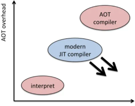
In the beginning of virtual machines, it interpreted intermediate code or compiled all intermediate code to native code during the Of-Time – we use a term Ahead-Of-Time (AOT) as a period JIT compiler is compiling or optimizing intermediate code, and program execution has not started. But in this manner its execution speed was much slower than that of a program compiled by static compilation. Mainly there are three reasons. First, execution speed of interpretation is slower than that of native code. Second, to compile all native code takes much time and this AOT overhead is vital issue for embedded application, because this overhead (i.e. user waiting time) directly affect user satisfaction. Lastly, for the same reason, JIT compiler cannot apply enough optimization for the program to avoid the increase of compilation time. Therefore it runs slowly.

From these reasons, JIT compilers have been improved along two main ideas – re-ducing the proportion of interpretation and the AOT overhead by compilation and opti-mization. Hence modern JIT compiler uses 2-step online compilation style. Firstly the program is compiled with no optimization or very light optimizations not to increase AOT overhead. Then only frequently executed methods (we call it as hot function or hot spot ) are applied costly optimization. Thanks to this compiling style, execution speed of JIT compiler is improved, and JIT compiler can greatly reduce the start up overhead. Now, main subject of JIT compilation studies is how it is realized to apply costly opti-mization without occurring significant overhead (see Figure 5). And Split compilation, described below, is expected to deal with this difficulty.

!" #$ %& '( )' *+ $ ','-./%0$12''+$ 304'(2('4$ !"#$ -%5236'($$ 5%+'(0$ 78#$-%5236'($

Figure 5: Now, JIT compilation studies tend to improve its execution speed without increasing

com-pilation or optimization overhead

2.3

Split Compilation

In general, for bytecode language executing system, each compilation role is assigned either to offline or online compiler. Usually platform independent roles (e.g. data-flow analysis, code verification etc.) are assigned to offline compilation, on the other hand target-specific optimizations and optimizations requiring run-time informations are done by online compilation.

In contrast, split compilation is realized by interaction between offline compiler and online compiler [3]. Split compiler divides a optimization process into two parts and one part is attributed to offline compilation and the other part is attributed to online compilation (Figure 6). Intuitively, the complexity of optimizations is moved from online compilation to offline compilation for reducing optimization overhead, and only a part of algorithm which requires run-time information stays on online compilation. As a result, the burden of that optimization algorithm on JIT compiler is reduced.

An annotation framework is one kind of interactions between offline and online world and it has good possibility to improve our implementation (see Section 9). For instance, when a static compiler compiles a statement, several bytecodes are generated with anno-tations and each bytecode has been optimized with taking into account several expected execution flows. And JIT compiler will chose the most effective one according to run-time information and its annotations. As a consequence, it will become possible for JIT compiler to apply more aggressive optimizations which cannot be applied for its expen-sive analyzing cost. For that reasons, split compilation gives us the best way of both offline and online world.

And the definition of split compilation can extend to all steps : offline compila-tion, linking, installacompila-tion, loading, online/run-time, and the idle time between different runs. Each phase of program gives a online compiler some useful knowledge of run-time environment (i.e. shared libraries, operating system, processor, input values). These

in-Figure 6: Split Compilation flow !" # $% &'( ") *( # +* ,$++-*.$* /"01!",2* 3%--&+* 1!",2* 4%561 !",2*

Figure 7: Optimization map (JIT compilation)

!" # $% &'( ") *( # +* ,$++-*.$* /"01!",2* 3%--&+* 1!",2* 4%561 !",2*

teractions between each program phase and online compilation are realized by additional information in intermediate code. For instance, using annotations or coding conventions. Thanks to the split compilation, online compiler can reduce its optimization overhead and apply very aggressive target-/context-specific run-time optimizations. Figure 7, 8 describe ”shift” of each optimization cost by split compilation. The optimization algorithms lying in the Low-cost area are applied during AOT compilation time, the ones lying in the Middle-cost area can be applied during JIT compilation time, and the others are never applied because of its expensive optimization cost (Figure 7). And Figure 8 shows the decrease of optimization cost over split compilation. This decrease makes it possible to shift one optimization algorithm to Low-cost area, and another one to Middle-cost area. Therefore it benefits especially embedded systems because they have limited resources and startup delay disapprovingly effects a user’s perception of program performance. Next, we show several studies which apply the idea of split compilation. Vectorization :

Rohou et al. [20] applied the notion of split compilation to bytecode vectorization. At first, during offline compilation, the scheme transforms source code to bytecode with optimization and adding the annotations which indicate which bytecode can be vec-torized. Then, during online compilation time, JIT compiler compiles the bytecode to native code which is suitable to SIMD vectorization. The point of their study is the application programmer can obtain the benefit of vectorization without concerning the target platform where the application is executed. These outcomes can be realized by costly and complex analysis during offline compilation time, and by interaction between offline compiler and dynamic compiler.

Global register allocation :

Krintz et al.[11] proposed annotation framework to realize the notion of split compi-lation. In general static information of the code, for instance local variables, control flow, exception handling etc., are gathered in offline. Their annotation framework communi-cate these analysis information to the compilation system. Thanks to this framework online compilation overhead is reduced, because this costly analysis is performed of-fline. And they applied this annotation framework to global register allocation. It is difficult to apply register-based optimization on Java program without costly analysis and algorithms, because Java byte code format is based on a stack frame architecture. Their approach statically counts the local variables to determine the priority of the local variables and stores that information in annotation. Then during online compi-lation time the annotations indicate which local variables have priority to be assigned to register. Similarly they also applied annotation frameworks to flow-graph creation, constant-propagation and inlining. Then their results shows reducing start-up delay up to 2.5 seconds.

3

Floating-Point Issues

Compiler developers not only propose new optimizations or analysis approaches but also must show the relevance of it. And they usually use benchmarks to make it sure. However there exist several cases that benchmarks cannot show real performance of compilers, and Rohou et al. [21] stress floating-point computation as a remarkable case. Floating-point representation is the most commonly used manner to treat infinite real numbers on computing systems with finite resources, since floating-point can represent wide range of numbers. Its wide representability is especially required in scientific com-putations. But one has to know that floating-point numbers may be an approximation to real numbers, because real numbers must be stored in memory in binary expression and generally real numbers cannot be exactly represented in finite binary expression. Hence there exist slight errors between real numbers and floating-point numbers, al-though which may not raise critical effect for computer programs in general. However, in the worst case, an error can accumulate into large one and it causes surprising results and unexpected behaviors.

In this section we show the complexity of floating-point and examples which easily cause mistakes or surprising results. And also we show the characteristics of fixed-point numbers as a contrast to floating-point numbers.

3.1

Floating-Point

Floating-point is very useful but sometimes it may cause unexpected results. But in general programmers need to manage it, because most languages have only float and double type to treat real numbers. The reasons why it cause incorrect results are very complicated, it depends on hardware platforms (IA32, x86 64, PowerPC etc.), compilers, and its definitions. Regardless floating-point is widely used, surprisingly, the definition of floating-point representation is not only one. But in this paper, we mention mainly IEEE-754 standard [8]. And end of this section we show a part of its definition.

Background of floating-point :

Floating-point is very widely used because of its rich representability. And in general floating-point is considered as it is exact representation of real numbers and results of its arithmetic operations are same across platforms. But these notions are mistakes. For instance floating-point is only an approximation of real numbers. It is derived from very simple reason such as computer have to treat infinite real numbers as finite binary expression (generally 32 bits or 64 bits). Therefore generally real numbers must have often rounding error in order to be stored in memory. These issues are well known to floating-point experts [12, 16], but they are not correctly understood by programmers. Examples of floating-point issue (and solutions) :

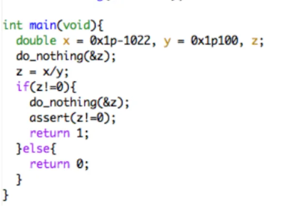
As we mentioned above, not all hardware platforms treat floating-point in a same manner. For instance, processors of IA32 architecture have 80-bit registers and floating-point can be treated as long double temporary on the registers in optimized code. And when a temporary is spilled to main memory the temporary will be split to 64-bit (same as IEEE-754 double precision). It causes reduction of precision and sometimes it causes unexpected behaviors. We show an interesting example from [16].

Figure 9: Zero no-zero example, compiled by GCC version 4.0.2 on IA32

This program can show three behaviors according to run-time configurations.

1. If it is compiled without optimization, main function returns 0. Because the value of x/y is stored in memory as IEEE-754 double precision number, and in this case the value is evaluated to 0 since the exact value of x/y is too close to zero.

2. If it is compiled with optimization, execution is terminated by assert statement. Since in this case the value of x/y is stored in register (i.e. 80-bit long double) and, conversely to IEEE-754 double precision, it is evaluated to non-zero because of its wide range precision. However after the test of if statement temporary z is spilled to memory (i.e. the value is rounded to 0), because compiler cannot know the behavior of do nothing function therefore compiler stores the value of z in local memory. As a consequence the test condition of assert statement fails.

3. If it is compiled in a same way as the last case except removing do nothing(&z) statement, main function returns 1. Because after the test of if statements tempo-rary z is not spilled to memory, for that reason z is evaluated to non-zero at assert statement.

This example shows a typical floating-point issue, and it depends on floating-point char-acteristic, hardware platform feature and even compiling optimization. And detecting all kind of these issues is very costly and time consuming.

The special values of floating-point, such as N aN (N ot a N umber) 1 _{and ±0} 2_{, also}

may cause some problems. For instance, although one can theoretically get the same results from next four expressions when they are computed over the real number, the results are not the same over the floating-point. However, and surprisingly, some com-pilers intentionally ignore the definitions of floating-point and apply unsafe optimization to improve its execution speed. For instance GCC, on SSE, with -O2 -ffast-math option compiles all these expressions in a same way as first row expression.

!""#""$"%""!"&"$" !"#'"$"%""!"&"$" !""(""$"%""$"&"!" !"('"$"%""$"&"!" !"'")*+"$"'",*" !"'"-.-+"$"'"/" ",*" )*" )*" ",*" """/" """/" "-.-" "-.-"

Figure 10: Second column and third column show the result over floating-point

As we showed here, there exist floating-point issues and each issues may depend on hardware platforms or compilers. Hence it is awkward problem especially for widely spread embedded applications, because programmers cannot know target hardware plat-forms when they design such applications.

Solutions :

There exists no solution which is valid to every architecture. But several approaches have been proposed to fix these issues, for instance GCC has

-ffloat-store option. It makes every floating-point variable be stored to memory. Using this option, we can avoid long double precision problems as we have shown ”zero nonzero” example. But it is clear that execution speed gets slow down. Moreover this option is valid only for variables (i.e. not including temporary), For that reason programmer have to manually rewrite the code to make temporaries be stored in variables. And it is time consuming and might cause new bugs. Hence Monniaux stresses in [16] that all compiler should include such options.

Another possibility is to force compilers to use SSE units3 for computation on IEEE-754 types. It seems simple solution for personal computers, but not all embedded sys-tems use processors equipped with SEE unit. In contrast Intel architectures, PowerPC architectures respect IEEE-754 floating-point arithmetic. However it requires software support to confirm with IEEE standard.

1_{NaN represents the result of operations which make no sense. e.g. 0/0, +∞ − +∞ etc.}

2_{Floating-point can represent sign of zero. It is useful when one treat the complex numbers.}

And we stress again that floating-point is very complicated and it may cause unex-pected results. However we have to manage them because most of programming language treat only float or double type.

Structure of floating-point :

Next, we show basic structure of floating-point to understand previous examples, and, to know detail, Goldberg synthesize well its definitions and issues in [7].

Floating-point numbers are represented as ±d.dd . . . d × βe _{(d.dd . . . d}× βe _{is called}

the significand) with a base β (which must be even) and a precision p. For instance, if one uses β = 10 and p = 3, the real number 0.5 is represented as 5.00× 10−1. In similar, if one use β = 2 and p = 3, the real number 0.5 is represented as 1.00× 2−1. And computers have to treat floating-point with β = 2, because any kind of values stored in memory must be binary expressions. For that reason, the decimal number 0.1 cannot be represented exactly, because it gets repeating fraction over the binary expression. Therefore floating-point represents it approximately (i.e. it is rounded, we mention it later.) as 1.10011001100110011001101× 2−4 (in this case p = 24). This is a main reason why a real number might not be represented exactly : the real number is represented in infinite repeating binary expression, even if the real number has finite decimal representation. And numbers whose value exceed the range of floating-point given p and β are treated as ±∞.

IEEE-754 defines two types of representation ; single precision type and double

pre-cision type. Single prepre-cision type is represented in 32-bit and satisfies p = 24,−126 <

log₂βe _{< 127 (see Figure 11). On the other hand double precision type is represented}

in 64-bit and satisfies p = 53,−1022 < log₂βe < 1023. And some architectures have extensive type long double type, however its format is not the same between architectures.

!"#$%&%'()!*++,-./%0+ #1!'(#(0)#*++2./%0+ &%3(/%0+4./%0+ 5+ ,6+ 65+ 64+++ ++ ++ ++ ++ ++ ++ ++ ++ ++ ++ ++ ++ ++ ++ ++ ++ ++ ++ ++ ++ ++ ++ ++ ++ ++ ++ ++ ++ ++ ++ ++

Figure 11: IEEE-754 single precision (32-bit)

Four rounding manners4 _{are defined by IEEE-754, and Round-to-nearest manner is}

the default and used in majority of programs. Round-to-nearest manner rounds a real value x to the floating value closest to x with the distance. If two floating-point value are equally close to x, the one whose least significant bit is equal to zero is chosen. However this manner hides double rounding issue. That is, rounding to nearest with different precisions twice in a row (for instance, real number → long double (on IA32 register)

→ double precision (on local memory) may cause different results from a result directly rounded to final type.

3.2

Fixed-point

In general, for programmers, using floating-point numbers (i.e. float or double type) is the only choice to represent real numbers. However it is not always true for hardware platforms. Next, we show an alternative representation of real numbers – fixed-point numbers.

Background of fixed-point :

In contrast floating-point representation, fixed-point representation always fixes bit-width of integer part and fractional part. For that reasons, fixed-point computation occurs fewer errors than floating-point computation, although it cannot represent as large real numbers as floating-point. Though there exist several notations to represent fixed-point, Q format is mainly used such as,

Q[OI].[OF ]

Where, QI = bit-width of integer part and QF = bit-width of fractional part (in binary expression ). And total bit-width is 1 + QI + QF : first 1 bit is used to specify sign. For instance, in Q4.3 format 12.625 is represented as ”01100101”.

As we have shown above, floating-point is complicated and its arithmetic computa-tions are more costly than fixed-point computacomputa-tions. For that reason, many processors have Floating-point Processor Unit (FPU) to reduce the cost of floating-point compu-tation. However some low cost microprocessors or microcontrollers are not integrated FPUs, and in that case the overflow of floating-point computations is not trivial.

Hence, sometimes fixed-point is preferred to floating-point for hardware platform in perspective of energy consumption an execution speed. But, in general, numerical precision is an afterthought for many programmers. For instance programmers often use double just because of its wide range representation, even if it is too precise and too costly for their program. Therefore, a conversion form floating-point into fixed-point is required for the purpose of improving execution speed and reduce power consumption. Next we show some studies of them.

Floating-point to fixed-point conversion :

As I mentioned above, sometimes floating-point need be converted into fixed-point, and at that time precision must be reduced otherwise to improve its performance. And it is very important to choose enough bit width (8-bit, 16-bit, 32-bit etc.) due to maximize the reduction of computation cost without inviting numerical precision errors.

In [15] Menard et al. proposed an automatic implementation framework which con-verts floating-point algorithms into fixed-point architectures under numerical accuracy

constraint. The method is divided into several processes, and chooses the most efficient bit-width and instruction sets with taking into account the interaction among each part they determine. And their framework showed significant reduction in the execution time compared to other conventional frameworks.

Linderman et al.[12] proposed analysis framework for conversion between floating-point and fixed-floating-point by improving Gappa [5] framework. They applied Affine Arith-metic extension to precisely analyze rounding errors, and their framework showed the effectiveness across real applications. And they also stressed that the precision analysis should be a part of programmers’ workflows.

Cong et al.[4] also proposed automated analysis framework of numerical precision between floating-point and fixed-point. They focused on the error coming from the truncation of values. From the experiments over three static analysis (Affine Arith-metic (AA), General Interval ArithArith-metic (GIA) and Automatic Differentiation (Symbolic Arithmetic), they showed Symbolic Arithmetic is preferred for expressions with higher order cancelations. Because AA and GIA can analyze well for first order cancelation effects, but cannot analyze sufficiently for higher order cancelations. On the other hand, Symbolic Arithmetic can analyze even higher order cancelations.

4

Conclusion : Bibliographic Study

Nowadays, embedded systems must be suitable to heterogeneous platforms without reducing its performance. And it is natural that bytecode language and JIT compiler were widely spread because of its distributability. Although JIT compilers enable target-and context-specific run-time optimizations, it is always under the restriction of limited resources and must keep compilation overhead low to reduce users’ waiting time. There-fore JIT compiler cannot apply aggressive and costly optimizations. Then we focus on split compilation. It is the best approach for embedded systems, since it can both keep optimization overhead low and apply aggressive optimizations through interactions between static compiler and JIT compiler such as annotation framework. In this pa-per we summarize the difference among static compilation, JIT compilation and split compilation with an introduction of split compilation.

In addition, we also show the issues of floating-point computation. It is very com-plicated and easily cause unexpected results. However these issues generally have been ignored by programmers, designers of programming languages and even compilers. Be-cause it is hard for static compilers to effectively manage the issues which may appear as consequence of execution context such as target hardware platform. And for JIT compilers it is too costly to analyze all possibility of that issues, and optimize it during execution time. However it is possible for split compilation, because split compilation can use both costly analysis information from static compiler and run-time information from JIT compiler.

floating-point computations, and what kind of informations can be optimal to improve the optimization. To achieve it, we believe the annotation framework can suitably adjust to a solution of a future work by combining aggressive static optimizations and dynamic timely optimizations. And as we mentioned above, programming languages do not give programmers a lot of options to treat the real numbers, in general only float or double. But in some cases, at runtime, it is better to convert floating-point into fixed-point or use less precise algorithm to improve execution speed. And we can also use annotations to know whether the convert or the change of algorithm are appropriate. Through these experiments, we reveal a necessity of the interaction between offline and online compiler.

Part II

Internship Report

5

Overview

As we mentioned in Part I, in several decades we will be able to use new generation embedded systems. It will hold heterogeneous multi cores up to several hundreds as many studies propose [2, 3, 19]. Therefore a new compilation method are strongly required. The method should give users the benefits of heterogeneous multicores without failing in a portability of applications.

But it is difficult to develop a high portability application over those heterogeneous devices, because we cannot know on which device the application will be executed. In addition we need to allocate the tasks to each core in correct manner to receive a maximum benefit of multicores. From this context we can say split compilation may have an important role, since it can apply aggressive optimization without losing its portability.

Parallel computing is a hot topic for the multicores processing, of course. However, in this internship we did not focus on increasing parallelization because of three reasons in terms of embedded systems. First, nowadays we cannot use several hundreds cores yet. We can use up to only several cores on actual embedded systems, although we have the perspective of huge multicores beeing stored on a device. Second, as Amdhal’s law shows5_{, it is very important to increase a percentage of parallelization area to get optimal}

results of parallel computing. To achieve it, it is the most important to decrease data dependencies of programs — we can call this as a software level constraint. Then, one needs to analyze data dependencies of a program in detail and may modify the program itself to reduce data dependencies. But this is out of our focus, because we want to apply our study for general programs instead of target specific programs. Lastly, we must take into account a memory structure of each hardware, because cache misses cause latencies. We can call this as a hardware level constraint in contrast to previous one. So, we have to tune a compiler to reduce this hardware constraint. In fact, our implementation are slightly optimized according to our environment, without customizing original target programs itself — we explain it in section 7.

Then we focused on optimization of sequential executions in perspective of speedup, especially floating-point computations. Because floating-point computations are time consuming and in some cases it is too high accurate computation. As a representative of floating-point computations, we studied mathematical functions which are included in math.h file. Because math functions are used in most of domains and not always we

5 _{Maximum speedup =} 1

(1−P )+P/N

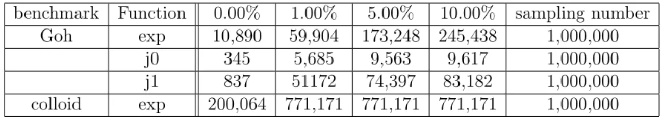
benchmark Function 0.00% 1.00% 5.00% 10.00% sampling number Goh exp 10,890 59,904 173,248 245,438 1,000,000

j0 345 5,685 9,563 9,617 1,000,000 j1 837 51172 74,397 83,182 1,000,000 colloid exp 200,064 771,171 771,171 771,171 1,000,000

Table 1: Samples of value locality : Each numbers explain the sum of the ten most frequently used

arguments. Each column corresponds to each error upper bound, in other words the arguments are more rounded in higher percentage. Goh is a program of ATMI benchmark suits and colloid is an example program of LAMMPS application.

need full bits of floating-point data structure — of course, there exist several pitfalls in floating-point computation (see Section 3), so one needs to care about it in case high precisions are required. So, instead of slightly canceling its accuracy we simplify math computations, as a result we accelerate floating-point computations.

Interesting numbers in Table 1 motivated us to promote the simplification of the math computations. The numbers express a total amount of the ten most frequently used arguments in some applications. For instance, from a number at the second low of the third column, we can say about 10% of the total computation of exp has done with any argument included in the ten arguments. That is, the table shows diversities of arguments passed to the math functions, in other words it shows how many times the same arguments has appeared in the program. Therefore the arguments has less diversity when each number has larger number. Each column corresponds to its upper bound of approximate computation — we mention how to approximately compute the math functions and estimate its error in Section 7.3.1. From this numbers, we can say the behavior of the arguments become less variety when the arguments are slightly rounded. For instance on j1 function of Goh benchmark, when the upper bound is 10.00% a total amount of appearances from the ten most frequently used arguments is 100 times higher than that of 0.00% case (i.e. actual values).

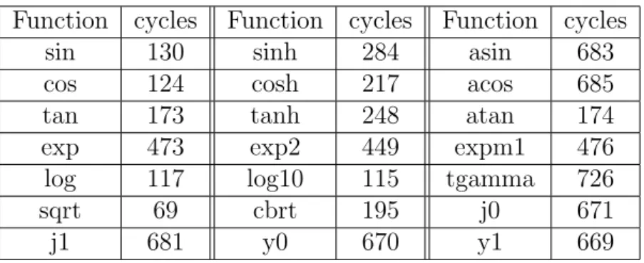
Table 2 shows execution clock cycles of each math function, from this table we can say sin, cos sqrt log etc. (approximately under 300 cycles function) do not have good potential, in contrast exp, asin, acos, j0, j1 etc. are rich computation in terms of clock cycles, so we mainly focus in these functions.

In our work, we applied data prediction and approximated math computation ac-cording to rounded arguments. Both methods have been well studied for long time. Especially data prediction is expected to overcome the limit of performance improve-ment depending on improveimprove-ment of CPU clock cycles.

The rest of this internship report is organized as follows. In Section 6 we mention related works of value prediction and approximation methods. In Section 7 we describe our methods during the internship. In Section 8 we show the results of our study. And in Section 9 we discuss our further work and conclude this internship report.

Function cycles Function cycles Function cycles

sin 130 sinh 284 asin 683

cos 124 cosh 217 acos 685

tan 173 tanh 248 atan 174

exp 473 exp2 449 expm1 476

log 117 log10 115 tgamma 726

sqrt 69 cbrt 195 j0 671

j1 681 y0 670 y1 669

Table 2: Clock cycles of each math function: These numbers explain clock cycles of each math functions

on Intel Core 2 Duo E6850 3.00GHz.

6

Related Work

Before explaining our method, we introduce several related works. Mainly we have two solutions — approximation computation and speculative computation.

By approximating mathematical functions, we can accelerate its computation instead of losing accuracy in reasonable range. Of course, approximated computation must cause additional errors more or less, but we have possibilities to do it in many cases. Because as we mentioned in part I of this paper, not always we need full precision of floating-point computations. That is, common program languages generally provide us only two value types (float, double) to manage real numbers. And most of non floating-point specialists use double type without analyzing truly required accuracy of their program because of a simple reason that double type is more precise than float type.

On the other hand, speculative execution is a effective method to reduce numbers of instructions or overcome data dependencies in loop statement by predicting next coming instructions. Therefore it is widely used from hardware level to software level, for instance reducing cache misses and eliminating true data dependencies directory lead to performance improvement especially in parallel computing. In this paper we introduce well known notions and methods like value locality, last value prediction, stride prediction, context based prediction, Markov prediction and global history buffer structure — and their hybrid methods. Moreover it does not cause additional errors in contrast to approximate execution. However as a drawback, it causes extra execution penalties when a speculative execution does not succeed, because we need to re-compute the set of instructions depending on the value of predicted instruction.

6.1

Function Approximation

Researchers of approximate computation are motivated a notion that one does not always want to compute the full accuracy result. This notion is not only for floating-point numbers but also fixed-floating-point numbers. In practice many approximation methods

were proposed over floating-point and fixed-point numbers [6, 23]. In general these notions are applied to hardware implementation to improve its performance in terms of execution speed, energy consumption and physical circuit area etc. For instance, Tisserand achieved 20%−50% speed up and 15%−30% silicon area reduction of circuits [24] with up to three order polynomial approximation. The study statically analyzes all candidates of coefficients for approximation by applying minimax binary search and estimates a relational error of the approximate computation after that the most moderate one is selected.

However these studies assume some restrictions like input range restriction or as-suming only monotonic math functions, and their target functions or input range are defined statically, because it is difficult to evaluate its computation error – in practice, we also restrict the area of approximation but it is defined in dynamic, not in static like these studies (see Section 7.3.1). In fact, in polynomial approximation, if one wants to increase its accuracy of approximate computation a higher order polynomial expression can provide smaller average error, though no one can determine an acceptable error up-per bound which can apply all applications But even in high order approximation some infrequent arguments can cause very large errors, and the error sensitivity depends on a target application.

Although in this internship we used linear approximation instead of polynomial ap-proximation, polynomial approximation may improve our performance. But in that case we need to statically analyze a target programs and passe that information (e.x. avail-able input range, moderate error upper bound to determine the appropriate coefficients.) to execution phase, for instance by the annotation frameworks [11].

6.2

Speculative Execution

First of all, most of related works we introduce here focus on integer numbers as tar-gets of their prediction value methods and implemented in hardware level. In contrast, we try to predict a value of floating-point variable passed to mathematical functions. Theoretically, int and float have same bit-width (32-bits) so total quantity of explainable different numbers is same. However, in some case, a usage of them is quite different, for instance integer numbers are used often as index of for loop or array. This is one of the most significant difference point between integer and floating-point numbers. More-over, the explainable range of double precision floating-point (64-bits) greatly expands compared to integer numbers, therefore the difficulty of prediction is greatly increasing. These differences are very important point when we focus on the predictability.

Data Redundancy

As a relevant study to collapse true data flow dependence in early days, S. E. Richardson proposed the concepts of trivial computation and redundant computation in [18]. Trivial computation is a concept that we have chance to transform a complex

instruction to an simpler one in some cases, for instance y = x/2 can be transformed to y = x >> 1. On the other hand, redundant computation is a concept that an operation can repeatedly performs the same computation to previous one.

Value Locality

Then M.H.Lipasti et. al. followed up the concept of redundant computation and proposed value locality [14, 13]. Their main idea is that keeping recently used values in the history table, after that when the same instruction is about to be executed one of the values in the history table is returned instead of executing actual instruction. Target instructions of the predictor is only data loading from memory in the first work, and in following work they applied the method to store instructions. Concretely their value prediction unit consist of two parts, which are value prediction unit and verification unit. In addition, value prediction unit consists of two parts, one is value history table and the other is a unit to decide whether prediction is triggered. And history table contains 4096 entries and decision unit has 1024 entries. As results, they exhibited 23% performance improvement as average (and up to 54%) in terms of execution speed.

Stride-/Contxet-based prediction and Hybrid Method

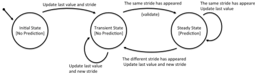
K. Wang and M. Franklin proposed stride predictor and pattern based predictor, and hybrid method of them [25]. Their main idea is monitoring the behavior a pattern of each instruction in order to achieve higher prediction rate compared to the last value predictor. As M. H. Lipasti et. al., their concept bases on value locality, for instance they exhibited that 15% - 45% of the instructions execute only a unique value in sixteen-wise value locality.

On one hand, stride predictor conserve the difference of values of each instructions, and when the same stride has appeared n times in a row (n-delta) the stride is validate and next value of the same instruction is predicted according to this stride. Unless the stride is validated, no prediction is done. Figure 12 describes the state chain of stride predictor. In effect 2-delta stride method achieved high predictability because of this concept is well fitting to predict loop index or array index values. On the other hand pattern prediction

!"#$%&'()%)*' +,-'./*0#1$-"2' 3/%"4#*")'()%)*'+,-'./*0#1$-"2' ()*%05'()%)*'+./*0#1$-"2' 670%)*'&%4)'8%&9*'%"0'4)/#0*' 3:*'4%;*'4)/#0*':%4'%77*%/*0' ' ''''''''''''''''<8%&#0%)*='''' 3:*'0#>*/*")'4)/#0*':%4'%77*%/*0' '670%)*'&%4)'8%&9*'%"0'"*?'4)/#0*' 670%)*'&%4)'8%&9*'' %"0'"*?'4)/#0*' 3:*'4%;*'4)/#0*':%4'%77*%/*0' 670%)*'&%4)'8%&9*'

consists of 2 units. One unit keeps 4 unique recently used values for each instruction (value history table), and the other keeps the pattern of the appearance of values with a score of a validity of the pattern (pattern history table). When a instruction is about to execute, prediction unit confirms whether the instruction is registered in the value history table and if so, the pattern history table evaluates the score of that pattern. Eventually when the score is greater than a user defined threshold, the next coming value is predicted. As experiments they compared their method to previous proposition[13, 14] and hybrid method of these predictors.

Their new prediction methods and hybrid methods work well, as a result they got 50% speed up in average and up to 80%. And remarkable point is its low incorrect pre-diction percentage (5% - 18%) as we easily understand from its miss prepre-diction tolerant mechanism described above. In contrast last value prediction showed less predictability and high incorrect prediction percentage.

In similar way, Y. Sazeides and J.E. Smith proposed context based predictor[22] and showed the prediction accuracy getting to 78%. In addition, they stressed the existence of 80%-20% rule even in terms of instructions and values generated by the instruction.

Markov Prefetch

Then D. Joseph and D. Grunwald proposed Markov prefetching method[10]. Their model consists of two parts, prefetch request queue and selection part of candidates for the queue, and the notion of Markov prediction is applied to selection part.

The global idea is whenever a cache miss has occurred that miss address is passed to prefetch table. That prefetch table has n-entries of miss address which reflects the history of cache miss and each entry has several candidates of next coming memory address with order of priority like as probability of Markov model. Then if the current miss address matches to a entry of the prefetch table, the most prioritized candidate of next coming address is sent to prefetch queue which follows FIFO and LRU policy.

Remarks of their implementation are, firstly, the target of prefetch is L2 cache because of modern out-of-oder processors successfully overcoming L1 cache misses latency. Sec-ondary, the prefetch queue called as prefetch buffer is separately located from L1 caches although the buffer is located inside of a processor. From this policy, Markov prefetch does not affect L1 cache in contrast to the conventional demand prefetch scheme. In fact, the conventional scheme stores fetch requests on the cache directly as a consequence spill out must occur and it may have side effect on the program performance. As drawbacks, Markov prefetch can only predict what has already appeared in the past in contrast with stride prefetch method.

From their simulation results, it was shown the accuracy of the Markov predictor globally adjusts to different kinds of benchmarks much better than stride predictor. In one case the hit rate is up to nine times higher than stride predictor.

Global History Buffer

By focusing on a different point from other studies, K. J. Nesbit and J. E. Smith achieved fine prediction accuracy with low memory resources thanks to a notion of Global History Buffer (GHB) [17], and also focused on L2 cache because of the same reason of Josep and Grunwald. Their contribution is proposing efficient structure of data manage-ment with their statical evidence rather than proposing brand new prefetch algorithm.

Their data structure has two tables — index table and global history buffer as in Figure13. Each entry of index table has a pointer to GHB and GHB preserves every

!"#$%&'($)*+,( -&,.,$/0(

1,'(

23$&'( _!"#$%&'(

-&,.,$/0(

)+4%&"$05( -&,.,$/0(()66&,##(

736,8($)*+,( -&,.,$/0( 1,'( 23$&'( -%"3$,&( 979 : ( ;+%*)+(!"#$%&'(<)*+,( -&,.,$/0(

)+4%&"$05( -&,.,$/0(()66&,##(

Figure 13: Table-based prefetch method : upper figure describes the conventional method and lower

one does global history based method.

value according to FIFO policy regardless differences of entries, when cache miss occurred prefetch key (PC or cache miss address etc) is passed to Index table, at the same time the prefetch key is inserted to the top of GHB. Thanks to this two steps reference scheme they successfully separate entry and history table and automatically evict old data from GHB. On the other hand, in the conventional methods, each prefetch entry always has a unique history table corresponding to each entry. As in consequence the prefetch data structure often consumes huge memory when one uses large entry size in order to increase the prefetch accuracy, additionally a proportion of useless data is not low. Because their statistics showed old cache is less frequently referred than young cache — an age of a data is the number of clock cycles since the data was last referred, for instance a data being younger than 4k has 10 times higher prefetch accuracy than a data being older than 16M. So, even if one conserves large history table for each prefetch entry, it may make no sense from macro point of view. As a result they got 20% ICP improvement

and up to 90% reduction of memory traffic.

6.3

Differences Between Previous Studies and Our Study

At first, the most significant difference is architecture-level implementation and software-level implementation. That is, we try to predict and manage data sets by software-software-level implementation in order to accelerate the execution, although previous works manage the cache, PC and memory address directly. From this point, we can say that we could manage the data set in simple and abstract, but we may still have some possibility to tune up our method in more primitive instruction level. The second different point is targets of prediction. Previous works target to standard instructions especially integer instruction like add, sub, multiplay etc., on the other hand we target to all arguments passed to math functions and its value. Obviously the search space of floating-point is much larger than the space of integer. In addition, there is less chance to detect favorable behaviors over floating-point numbers in contrast to integer numbers, like for loop index and array index. Therefore prediction the floating-point numbers is really challenging. Lastly, most of previous works aim to collapse true data dependency for the sake of improving parallelization, on the other hand we try to accelerate sequential execution itself. In other words, when we successfully achieve the improvement we can combine these two methods to benefit from each strong points.

In following section, we explain a concept of our study and its mechanism.

7

Our Study

7.1

Concept of Dynamic Linked Pseudo Math Library

As we wrote in Section 5, our main purpose is how to accelerate mathematical com-putations from split compilation’s perspective (i.e. on embedded systems). However, this study was done on the desktop environment as a prior study to understand a po-tential of our concept. From this context, we cannot modify a target source code itself nor analyze the target source code in advance, a JIT compiler cannot know which kind of application is executed on the device and how it behaves.

To over come these constraints we propose Dynamic Link Pseudo Math Library. This library is inserted between an application and true math library 6 _{then it is called}

6_{when we execute a binary code, we set and export an environment variable LD P RELOAD as}

whenever any math function is about to be executed and behaves like true math library. However, the library does not always compute math functions in normal way. The library profiles arguments passed to a target math functions and attempts to predict the value or approximate the computation in similar way to related work. The purpose is to reduce costs of math function computations, by prediction or approximation. Figure 14 simply describes this mechanism.

!"#$"%& '& '& ()*+!(&,-.)*/&012!& !"#$%&'( !"#$"%& '& '& ()*+!(&,-.)*/&012!& )&*+,'%!"#$%&'( !"#$%&'( -./**(0.'"0*&( 34#*!2-051.& 64)##*1"-7)51.& 84(*9!&017#9()51.& :&;<=>?@;AB<&:& 1'/$2!(*3*0+4'5( 6+/($*7.',(

Figure 14: Overview : Pseudo math library has

three choices; prediction, approximation and true

computation. The library is always called before

real math library is called.

!"#$"%& '& '& !"#$%!&'()"#*&+,-%& ./#%%&+/,(+%0& ()#*!+,-./0& 1)2##*/",32./0& 4)5*6!&-/3#652./0& 10%2-,34('530,& 7&89:;<=8>?9&7& 6"()&!/#%"-& 789&:& 6"()&#,4%& ();*/@A,0B& 1);2CC,0B&#*!+,-5!+& D2A6!5/&32,0&5E*!2+& ;%41%#&!/#%"-& 789&<&

Figure 15: The target program and main thread

of the pseudo library is executed on CPU1. CPU2 executes only helper thread of the pseudo libary.

To achieve our purpose, it is important to profile in efficient way and not to cause negative effect on the execution. Then, to separate the role such as math function execution and data profiling, we use two threads — main thread and helper thread, respectively. In our study, we use Intel Core 2 Duo processor and main thread and helper thread are allocated to different CPU, therefore each thread can use all local CPU resources (register, L1 cache and CPU time) and does not affect the performance of each other7_{. The main thread executes a target program and if math function is called,}

it decides how to compute the target math functions. On the other hand helper thread profiles the history of arguments of each target math function, and supplies appropriate candidates for approximation or prediction in the main thread. The helper thread never executes the target program itself, contrary to the main thread (Figure 15).

Besides we introduce notions of data block, ownership and masking method to im-prove the performance, former two notions are described in Section 7.4 and latter one is described in Section 7.3.

7_{In terms of cache coherence of shared data, the coherence protocol can affect the performance —}

this problem is mentioned in Section 7.4. However each CPU time is all ways allocated to one thread, never allocated to two threads on the same CPU.

7.2

Main Thread

The principal roles of main thread are communicating with an application program and deciding how to compute a math function, as described in figure 16.

!"#$%&'()%*+&,#('-+.% /,,"010&'-+.% /%&'()%2#.*-+.%03%% *'44$5%0.%('"6$(%',,40*'-+.% % 7"$50*-+.% 8)$*90.6%()$%,"+:40.6%0.2+"&'-+.% 3#,,40$5%;<%)$4,$"%()"$'5% ='&,40.6%()$%'"6#&$.(% '.5%3$.50.6%0(%(+%3#;%()"$'5% "$(#".% >#56$?% ,"$50*-+.% ',,"+10&'-+.%>#56$?% !"#$ !"#$ %&$ %&$ '()*+,-$

Figure 16: The execution flow chart of main

thread. !" #$%&'()*" +)%,"-.$/01$" *#$&)'")22'1!#+)01$" 3" '&-&'&$/&"21#$%"

Figure 17: Linear approximation : The gray circle

is the reference point (x0) and if an argument (x,

the diamond) is in the predicted range (i.e. x0<=

x < x0+interval) the main thread return a result of

linear approximate computation (the white circle).

As a former role, the main thread communicates with the target program as follow-ing. Firstly, the main thread is called whenever a target math function is called in the program. Secondary, it keeps arguments which were passed to the target math function. Finally, it sends the sampled argument to the helper thread. The target math functions are set in advance (i.e. statically defined).

As a latter role, the main thread decides how to compute the math function with taking into account the information analyzed in helper thread. All the information for prediction and approximation are prepared by the helper thread, therefore the main thread just decide whether the main thread tries to approximate or predict, referring to the analyzed information produced by the helper thread. Thanks to this process, the main thread has less overhead to make a decision.

Next, we simply mention how the main makes a decision to prediction or approx-imation. Firstly about the prediction process, the helper thread profiles the sampled arguments and predict the arguments which will be passed to the target function and pre-compute the value of the function. Then, if the predicted argument really appears, the main thread return the pre-computed result. Secondary about the approximation process, the helper thread also predicts the range where values of the arguments will be included. The helper thread supplies the size of the range and the reference point of the range. Then the main thread checks whether a new argument passed to the target

function is included in the range, and if so, the main thread applies linear approximation to the target function like in Figure 17. In that case, all necessary coefficients are also supplied by the helper thread, and these coefficients are defined not to exceed an error upper bound. We mention it in following section.

7.3

Helper Thread

As we mentioned the role of the helper thread in Section 7.1, a main purpose of the helper thread is to supply informations for predicting a behavior of target math functions to the main thread. The prediction distinguishes two types : a true prediction and a range prediction. The true prediction simply predicts an argument being executed by the target math function and a value of that computation. On the other hand the range prediction predicts a range where the arguments frequently used are included, because the arguments included in this range also may be frequently used from now on according to value locality [14, 13]. When the target math function uses an argument included in the predicted range, the main thread approximately computes a value of the function instead of computing the value in normal way.

To achieve the purpose, the helper thread has two phases; a profiling phase and a prediction phase, which are mentioned in Section 7.3.2 and Section 7.3.3 respectively. Besides, we mention a masking method in following section before moving to explanations of these phases. The masking method is a core idea to effectively manage floating-point numbers.

7.3.1 Masking Method and Error Computation

Since arguments passed to math functions vary, it is difficult to predict the argu-ments. However as we saw in Table 1 when the arguments are slightly rounded the be-havior becomes less complex. For this reason, the helper thread mainly manage rounded arguments. Accordingly, we mention how to round the arguments and compute error upper bound of the rounding in this section.

The masking method is bit canceling computation adjusted to double precision floating-numbers. Mask has 64 bits and we can set statically n-zeros in a row from a bottom bit up to 52bits (i.e. mantissa bits), then we compute ’and’ operation to the argument as Figure 18, 19. We call this mask as static mask in contrast to dynamic mask we mention later.

Masking method has two advantages, firstly it is faster to round the argument com-pared to relational operator (<, <=, >, >=) because when we use the relational operators it needs to compute twice (for a upper bound and a lower bound). Secondary, we need not be concerned about digits of the arguments because the digits are automatically computed in exponential bits. However in relational operator it is difficult to decide the upper bound and the lower bound in reasonable sense because the digits can vary.

!"!!#!!#!!#!!"!!#!!"!"!!#!!#!!#!!#!!"!"!#!#!"! !#!!#!!#!!#!#!!#!!"!"!!"!"!!"!!"!!"!"!"!"!"! $%&'()*+! ($,-! !"!!#!!#!!#!!"!!#!!"!"!!"!"!"!"!"!"!"!"!"! %.'*/)/!$%&'()*+! ・・・! ・・・! ・・・! 0!

1!

Figure 18: Masking (n = 11) : All bits which are

not described in the figure have ’1’ in mask bits se-quence. Therefore the rounded argument conserves its original bits sequence in higher than 11th bit.

!"

!"

・・・" ・・・" ・・・" ・・・"

#$%&'()*"

+),-#$."

Figure 19: Simple image of rounding over x axis

: Arguments converges to the reference points (the gray circles) by rounding operation. And we call a distance between each reference point as interval.

When we compute a math function by linear approximation, we have to manage an error of the approximate computation and want to confirm the error does not exceeds an error upper bound which is defined statically in our study. However it is quite time consuming to detect an actual maximum error point every time (note that, we apply the approximation several millions times or even several ten millions times during whole execution.). For this reason, an error of our approximate computation is defined as the maximum relational error among three quarter points as described in Figure 20.

!" ##" ##" ##" ##" $%&'()*+" ,*&-"./%012%" +$%'*("*33(2!$,*12%" 4" 45" 46"

Figure 20: We approximate a math

function between two reference points (the two circles). And a error is defined as the maximum relational error among three quarter points (the diamonds). In

this case, the error is|(|y2− y1)/y1||.

!" #$%&'()*""+,%)-./" ,%)-."0),1")22'3!#0)-3$" '&4&'&$.&"23#$%" 56$)0#."0),1")22'3!#0)-3$" $&7"#$%&'()*""+56$)0#./"

Figure 21: When statical approximation error exceeds the

error upper bound, dynamic mask recomputes the interval (the two black circles) to confirm that a new maximum error does not exceed the upper bound (the upper bound is statically defined).

But the relational error must be greater than 1 (i.e. over 100% error) when signs of an approximate result and a true result are opposite like Figure 22, because of the

!" #$%&"'()*+,)" -.)/$0"$110,!.#$+,)" 2" 23" 24" !3" !4" /!*//5.)6"7,)/" .)%/08$-""952)$#.*$--2"5/:)/5;"

Figure 22: When the approximate computation is done with an argument included in exceeding zone,

its relational error must exceed 100% error. Therefore whenever results of true math function at x0

and x1 have opposite signs, that dynamic mask is abandoned to ensure its error does not exceed the

maximum upper bound.

definition of the relational error. And when none of the three quarter candidates we mentioned above is not included in this area, the helper thread cannot detect that the approximation can exceed the error upper bound until it computes a value with an argument included in this area. To avoid that situation, when the helper thread finds results of math function with x0 and x1 have opposite sing, the helper thread abandons

that dynamic mask to ensure the approximate computation does not exceed the error upper bound.

Thanks to the masking method, we can easily sample the floating-point numbers. However the static mask cannot confirm the results of the approximate computation are lower than the error upper bound, although it can round the arguments in constant proportion regardless the digits of the argument. Then we apply a dynamic mask method. The dynamic mask is defined as follows. At first we reuse the interval of static method and its middle point — we regard it as a reference point of dynamic masking. Then, we search a maximum mask within the error upper bound. The error is computed in same way as Figure 20. As a result, an interval of dynamic mask can be either smaller or greater than that of static mask (Figure 21), since when static approximation exceeds the error upper bound we need to compress the approximation error under the upper bound. And also we can expand the interval when the static approximation error is too small compared to the upper bound, for the sake of maximizing a benefit of the approximation. In short, we use static mask for sampling the arguments to simplify the process and dynamic mask to confirm the relational error upper bound.

7.3.2 History Table

Here, we explain a profiling process. The profiling process consists of two parts — sampling and evaluation as described in Figure 23. During the sampling process, the helper thread receives an argument from main thread every time the target function is called in the program. And the helper thread does static mask operation to the argument,

then the masked arguments are stored in a n-entry history table according to an index returned by a hash function. Each row of the history table contains three elements — masked argument, score and recentness. The score explains how often the argument is used with taking into account its recentness. The recentness records when the arguments appeared last time.

!"#$%&'()*!! !!!!!!+,#-&!&".(!)/#'"01! *)"23! &"*4! /"*/! !"#$%&'($)*+,( -%.(&)/0($)*+,( 5#'63-&5%)"2-(!! ,-#!! 7.('"#!"55#-8.&"2-(! +,-#!&".(!)/#'"01! "!*')!-,! .(,-#&"2-(! '9"7%"2-(! *"&57.($!

Figure 23: The sequence of the profiling in the helper thread

After every period of time the history table is evaluated. Firstly the helper thread evaluates the recentness of each entry and an entry decreases its score if its argument has not appeared in that period. Then, according to a descending order of the scores, m arguments are stored into a top rank table and these arguments become the reference points for the linear approximation after being done the dynamic masking. For each top argument, the helper thread prepares the reference point, coefficients for linear approx-imation and dynamic mask. After that, the helper thread sends the information to the main thread.

7.3.3 Markov Prediction

Our prediction method follows the Markov prediction [10] over the Global History Buffer [17]. That is, the GHB keeps recently sampled actual arguments and their masked values as a reference point when the helper thread searches the table. In addition the GHB does not have huge entries and respects FIFO policy to avoid stale arguments . As we described in Figure 13 we need the index table to trigger the prediction process, in our study the top rank table behaves as the index table. The prediction process is as follows. Firstly when a new argument is thrown from the main thread, the helper thread inserts its statically masked value (we call it as masked argument) into the history table and also into the GHB. Next, the helper thread checks whether the same masked argument exists in the top rank table, if so the helper thread starts to search it in the GHT.