Essais sur l'exploitation d'un stock commun de ressource naturelle par des agents hétérogènes

Université de Montréal

Essais sur l’exploitation d’un stock commun de

ressource naturelle par des agents hétérogènes

par

Hervé Lohoues

Département de sciences économiques Faculté des arts et des sciences

Thèse présentée à la Faculté des études silpérieures en vue de l’obtention du grade de Phi1osophia Doctor (Ph.D.)

en sciences économiques

Mars 2006

Université

1I

de Montréal

Direction des bibliothèques

AVIS

L’auteur a autorisé l’Université de Montréal à reproduire et diffuser, en totalité ou en partie, par quelque moyen que ce soit et sur quelque support que ce soit, et exclusivement à des fins non lucratives d’enseignement et de recherche, des copies de ce mémoire ou de cette thèse.

L’auteur et les coauteurs le cas échéant conservent la propriété du droit d’auteur et des droits moraux qui protègent ce document. Ni la thèse ou le mémoire, ni des extraits substantiels de ce document, ne doivent être imprimés ou autrement reproduits sans l’autorisation de l’auteur.

Afin de se conformer à la Loi canadienne sur la protection des renseignements personnels, quelques formulaires secondaires, coordonnées ou signatures intégrées au texte ont pu être enlevés de ce document. Bien que cela ait pu affecter la pagination, il n’y a aucun contenu manquant.

NOTICE

The author of this thesis or dissertation has granted a nonexciusive license allowing Université de Montréal to reproduce and publish the document, in part or in whole, and in any format, solely for noncommercial educational and research purposes.

The author and co-authors if applicable retain copyright ownership and moral rights in this document. Neither the whole thesis or dissertation, nor substantial extracts from it, may be printed or otherwise reproduced without the author’s permission.

In compliance with the Canadian Privacy Act some supporting forms, contact information or signatures may have been removed from the document. While this may affect the document page count, it does flot represent any loss of content from the document.

faculté des études supérieures

Cette thèse intitulée:

Essais sur l’exploitation d’un stock commun de

ressource naturelle par des agents hétérogènes

présentée par: Hervé Lohoues

a été évaluée par un jury composé des personnes suivantes: Yves Sprumont président-rapporteur Cérard Caudet directeur de recherche $idartha Cordon membre du jury Hassan Benchekroun examinateur externe Yves Spru;nont

représentant du doyen de la FES

RÉSUMÉ

Cette thèse est composée de trois chapitres portant sur l’exploitation d’une res source naturelle commune par des agents hétérogènes. Les problèmes d’exploita tion d’une ressource naturelle commune sont généralement modélisés par des jeux différentiels dans lesquels il est tenu compte des hteractions stratégiques entre les agents et aussi de l’impact de leurs actions sur la dynamique de la ressource. Ce travail apporte une double contribution à la littérature portant sur ce sujet. Premièrement, nous introduisons une double asymétrie dans les deux modèles d’agents hétérogènes que nous présentons et nous caractérisons explicitement des équilibres avec des stratégies en boucle fermée. Deuxièmement, nous analysons les effets des cieux types d’asymétries sur les équilibres qui en découlent, dans un contexte d’équilibres markoviens parfaits. Dans le premier chapitre, nous nous restreignons aux stratégies markoviennes linéaires (stratégies exprimées comme une _{proportion du stock courant de la ressource) et déterminons les conditions} nécessaires d’utilisation de telles stratégies. Dans le second chapitre, nous sup posons que _{les conditions établies au premier chapitre sont vérifiées et nous ca} ractérisons explicitement des stratégies markoviennes linéaires pour un modèle de « f ish ‘War » dans lequel interviennent deux groupes d’agents différant par leurs taux d’actualisation. Dans ce premier modèle, les agents se font la concurrence seulement pour l’exploitation de la ressource. Nous examinons par la suite l’im pact du différentiel de taux d’actualisation et de la répartition des agents sur les équilibres obtenus. Dans le dernier chapitre, nous présentons un modèle d’exploi tation d’une ressource naturelle commune avec des agents repartis en deux groupes et différant par leurs coûts marginaux. Dans ce second modèle, les agents se font la concurrence aussi bien pour l’exploitation de la ressource, que pour la vente de leur production sur le même marché. Nous examinons les effets du différentiel de coûts marginaux et de la répartition des agents sur les équilibres obtenus. Pour les deux

modèles, nous trouvons que les deux types d’asymétries affectent effectivement les équilibres obtenus.

De façon plus spécifique, dans le premier chapitre, nous caractérisons les condi tions nécessaires permettant l’utilisation de stratégies markoviennes linéaires dans les jeux différentiels décrivant l’exploitation d’une ressource naturelle commune. Nous montrons que l’existence de tels équilibres est assujettie à l’existence d’une relation précise entre les éléments essentiels du modèle, notamment la fonction d’utilité des agents et la fonction de « dynamique naturelle » ou de reproduction de la ressource exploitée. Ainsi, pour une fonction d’utilité domée, seule une fa mille spécifique de fonctions de reproduction est compatible avec l’utilisation de stratégies markoviennes linéaires. De même, lorsque la fonction de reproduction est connue, seule une famille particulière de fonctions d’utilité permet l’utilisatioll de stratégies linéaires.

Dans le second chapitre, nous étudions un « fish War » dans lequel les agents impliqués se font la concurrence uniquement sur le marché de l’intrant, c’est-à-dire uniquement au cours de l’exploitation de la ressource. Ces agents sont repartis en deux groupes et diffèrent par leur taux d’actualisation. Nous examinons l’impact du différentiel de taux d’actualisation sur l’équilibre de ce jeu. Nous montrons alors qu’au niveau global, des augmentations du différentiel de taux d’actualisation et de la proportion d’agents avec le taux d’actualisation le plus élevé (les « gros »), augmentent l’extraction totale et diminuent le stock de ressource à l’état station naire. Cependant, au niveau individuel, l’impact de ces deux types d’asymétrie dépend de la comparaison de l’élasticité de l’utilité marginale à un. Pour ce qui est de l’asymétrie de « taille de groupe », lorsque l’élasticité de l’utilité marginale est supérieure (inférieure) à un, une augmentation de la proportion de « gros » agents dans l’industrie, tend à réduire (augmenter) le taux d’extraction des deux types d’agents. Ainsi, chercher à rendre l’industrie plus « homogène » en « gros » agents aura tendance à atténuer (exacerber) la « guerre » engeidrée par la concur

V

rence, lorsque l’élasticité de l’utilité marginale est supérieure (inférieure) à un. Concernant l’asymétrie de taux d’actualisation, une augmentation du différentiel augmente toujours le taux d’extraction des « gros » agents. Par contre, pour les « petits » agents, cette augmentation du différentiel de taux d’actualisation tend à réduire (augmenter) leur taux d’extraction lorsque l’élasticité de l’utilité marginale est supérieure (inférieure) à l’unité.

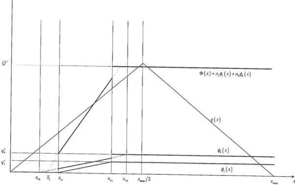
Dans le dernier chapitre, nous considérons deux groupes d’entreprises qui ex ploitellt une ressource naturelle commune et en vendent la production sur le même marché. Dans ce cas, ces entreprises se font la concurrence aussi bien sur le marché de l’intrant que sur le marché de l’extrant. Deux entreprises représentant chaque groupe diffèrent l’une de l’autre par leurs coûts marginaux. Nous avons ainsi un groupe d’entreprises à bas coût marginal auxquelles nous feront référence en tant que « grosses » entreprises, et un groupe à haut coût marginal que nous présenterons comme étant les « petites » entreprises. Nous caractérisons explici tement les stratégies markoviennes d’équilibre de ce jeu, ainsi que les effets des deux types d’asymétrie sur les équilibres obtenus. Les stratégies d’équilibre sont caractérisées par trois intervalles de stocks de ressource sur lesquels les entreprises adoptent des comportements différents. En-deçà d’un certain stock-seuil, aucune entreprise ne produit. Entre ce stock-seuil et un second stock-seuil, les entreprises exploitent la ressource à des taux linéaires et croissants avec le stock de ressource. Au-delà de ce second stock-seuil, les entreprises exploitent la ressource à des taux constants et qui correspondent aux taux d’exploitation qu’elles auraient adoptés si elles se faisaient une concurrence statique à la Cournot. Nous trouvons que la présence d’asymétries induit des discontinuités dans la strat.égie des grosses entre prises, et par conséquent dans le taux d’exploitation agrégé. Nous montrons aussi que le stock-seuil à partir duquel les petites entreprises commencent leur exploita tion et le stock-seuil à partir duquel elles adoptent leur exploitation à la Cournot statique, sont tous les deux plus élevés lorsque ces entreprises sont en présence de

grosses entreprises (cas asymétrique) que lorsqu’elles sont toutes identiques (cas symétrique). Quant aux grosses entreprises, lorsque leur proportion dans l’indus trie dépasse un certain seuil, le stock-seuil auquel elles commencent l’exploitation est plus élevé dans le cas symétrique que dans le cas asymétrique. En-deçà de ce seuil, ces grosses entreprises commencent leur exploitation à un stock-seuil plus bas que dans le cas symétrique. Le stock-seuil auquel elles adoptent leur comportement à la Cournot statique est, quant à lui, toujours plus bas dans le cas asymétrique que dans le cas symétrique où elles sont toutes de grosses entreprises. Nous trou vons aussi que ce modèle admet un ou trois états statiollnaires selon la valeur du différentiel de coût marginal ou la répartition des entreprises. De plus, chacun de ces états stationnaires peut être obtenu en faisant varier les deux types d’asymétries.

Mots clés: ressource naturelle commune, oligopole, jeu différentiel, stratégie markovienne, équilibre en boucle fermée, agents hétérogènes, asymétrie.

$UMMARY

This dissertation is composed of t.hree essays dealing with heterogeneotis agents exploiting a natural resource owned incommon. Problems of common pool resource

harvesting are often modelled as differential games, which take into account the strategic interactions between the agents involved and the dynamics of the resource. Our present work brings two main contributions to this literature. Firstly, we introduce asyrnmetry among the agents and derive explicit closed-loop equilibrium strategies for the asymmetric model obtained. $econdly, we examine the impact of these asymmetries on the outcomes of the game, that is, on the individual strategies of the agents, on the aggregate extraction rate and on the equilibrium steady states, in the context of Markov perfect Nash equilibria. In the flrst chapter, we restrict attention to linear Markov strategies (strategies expressed as a constant proportion of the current resource stock) and derive necessary conditions for the use of such strategies. In the second chapter, we assume a model that satisfies the conditions derived in the first chapter and solve for explicit linear Markov strategies for a “fish war” involving two groups of agents of different sizes with different discount rates. In this fish war modeL agents compete oniy on the input market. We then examine the impact of the discount rate differential and the distribution of the agents on the equilibrium outcomes of the game. In the third chapter, we present a common pool resource game witli two groups of agents (firms), competing this time on both input and output markets. In this last chapter asymmetric ftrms differ by their marginal costs. We examine the effects of the marginal cost differential and the distribution of the two types of firms on the outcomes of the game. We find that, in both models, both types of asymmetries affect the outcomes of the games in

important way.

To be more specific, in the first chapter, vie derive necessary conditions for the existence of Markov perfect Nash equulibria in linear strategies for common pool

resource differential games. We show that for such strategies to be used, a precise relationship must 5e satisfied hetween the primitives of the inodel, namely the utility function of the agents and the growth function of the resource. Thus, for a given utility function. only a specific family of growth functions is compatible with the use of lillear Markov strategies. Conversely, for a given growth function, only

a precise farnily of utility functions allows the use of such strategies.

In the second chapter, we present a “fish war” between agents exploiting a common pool resource and divided into two groups of potentially different sizes. Agents are identical within a group but differ between groups by their discount rates. _{We examine the impact of discount rate and group size asymmetries on} the outcomes of the game. We show that, at the industry level, increases in the discount rate differential and in the proportion of “big” agents (those with the larger discount rate), both increa.se the aggregate extractioll rate and decrease the steady state stock level. However, at the individual level, the impacts depend on whether the elasticity of marginal utility ïs greater or smaller than unity. For the csize asymmetry, when the elasticity of marginal utility is greater (smaller) than

unity, an illcrease in the proportion of big firms tends to decrease (increase) the

individual extraction rates of both types of agents. This means that, making the industry “more homogeneous” in big agents will tend to attenuate (exacerbate) the “flsh war”, if the elasticity of marginal utility is greater (srnaller) than one. As for the discount rate asymmetry, an increase in the discount rate differential aiways increases the individual extraction rates of the agents with the larger discount rate. However, when the elasticity of marginal utility is greater (srnaller) than unity, this increase in the discount rate differential decreases (increases) the extraction rates of the agents with the smaller discount rate.

In the last chapter, we consider two groups of firms harvesting a common pool resource and selling their production on the same output market. They therefore compete on both the input and the output markets. Representative firms of these

ix

two groups (of potentially different sizes) differ from orie another by their marginal costs. We then have a group of low marginal _cost firms

— referred to as “big” firms — and a group high marginal cost firms

— referred to as “small” firms. We derive explicit Markov perfect equilibrium strategies auJ examine the effects of marginal cost clifferential and group size asy;nmetries on the outcornes of the game. The

equilibrium strategies of the firms are characterized by three intervals of stocks over which they adopt different exploitation behavior. When the resource stock is less than a certain threshold, there is no exploitation at ail. Above that threshold and below a second threshold, the firms exploit the resource at rates that are linear auJ increasing in the resource stock. From this second threshold on, the ftrrns produce at the constant harvest rates they would adopt under a static Cournot game. We find that the presence of asymmetries induces discontinuities in the strategy of the big firms and consequently in the aggregate harvest rate. We also find that the srnall low cost firms begin exploiting the resource and revert to their static Cournot production at threshold resource stocks that are hïgher when they are in presence of big ftrms than when they are the only type in the industry. As for the big low cost firms, they hegin exploiting the resource at a higher resource stock in the asymmetric case than in the symmetric case when their proportion in the industry is above soine threshold, auJ at a lower resource stock when their proportion is below that threshold. They begin producing at their static Cournot harvest rate at a lower resource stock in the asymmetric setting than in the symmetric setting. We also find that the equilibrium outcomes admit one or three steady states depending on the range of the asymmetries. Moreover any of these steady states can be reached by varying the asymmetries.

Keywords: common pool resource, oligopoly, differential garne, closed loop equilibrium, Markov strategies, heterogeneous agents, asyrnmetry.

TABLE DES MATIÈRES

RÉSUMÉ

SUMMARY .

vii

TABLE DES MATIÈRES LISTE DES FIGURES

X xii DÉDICACE REMERCIEMENTS xlii xiv 1.2 The model 1.3 1.4 1.5 1.6

Admissible growth functions, given a utility function

Admissible utility functions, given a growth function An extension

Concluding remarks CHAPITRE 2: GROUP AND

WAR 2.1 Introduction 2.2 The model

2.3 Effects of the asymmetries

20

21

23 29

INTRODUCTION GÉNÉRALE.... ₁

CHAPITRE 1: ON LIMIT$ TO THE USE 0F LINEAR MARKOV STRATEGIES IN COMMON PROPERTY NATU

RAL RESOURCE GAMES ₈

1.1 Introduction ₉ 9 12 14 16 19 A FISH SIZE ASYMMETRIES IN

xi

2.3.1 Impacts of “size” asymmetry ₃₀

2.3.2 _{Impacts of “intrinsic” asymmetry 31}

2.4 Concluding summary ₃₃

CHAPITRE 3: ASYMMETRIES IN A COMMON POOL RESOURCE

OLIGOPOLY ₃₅

3.1 Introduction ₃₆

3.2 The model ₃₉

3.3 Characterization of an equilibriuin ₄₁ 3.4 Effects of the Distribution of Firms ₄₆

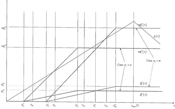
3.4.1 _{Comparing nb} n and n8 = n ₄₇

3.4.2 _{Comparing O <n8 <n and n5} = n _4$ 3.4.3 Comparing O < nb <n and nb n ₄₉

3.4.4 The Aggregate Harvest Rates ₅₁

3.5 Steady States ₅₁

3.5.1 _{Type and Nuniber of Steady States 53}

3.5.2 _{Asymmetries and Steady States 57}

3.6 Conclusion ₅₉ 3.7 APPENDIX ₆₁ 3.$ Figures ₇₆ CONCLUSION GÉNÉRALE ₈₉ BIBLIOGRAPHIE 92

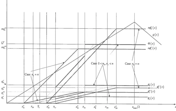
3.1 Equilibrium Strategies and Aggregate Outeome when O < n5, nb < n 76

3.2 _{Equilibrium Strategies and Aggregate Outcomes when n5 n and}

nb=n ₇₇

3.3 _{Equilibrium Strategies and Aggregate Outeornes when O < n5 < n}

and n5 = n ₇₈

3.4 _{Equilibrium Strategies and Aggregate Outcomes when O < nb < n}

and n1, n ₇₉

3.5 _{Equilibrium $trategies and Aggregate Outcomes when O <}

b <n

n5 = n and nb = n ₈₀

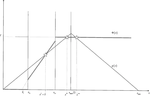
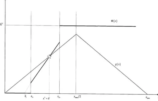
3.6 Steady States when x15 < < x25 and g (mx/2) QC•

Three

$teady States (Ail Regular) ₈₁

3.7 Steady States when fr15 < î < 25 and g(max/2)

<Qe.

Que Steady

State (Regular) ₈₂

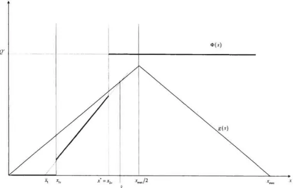
3.8 $teady $tates when x25 and g (iniax/2) QC. _{Three $teady}

States (Que Irregular) ₈₃

3.9 $teady States when > _{and g (rnax/2) <}

Qc.

_{Que Steady State}

(Irregular) ₈₄

3.10 Steady States when x15 and g(max/2)

Qc.

Three Steady

States (Que Irregular) ₈₅

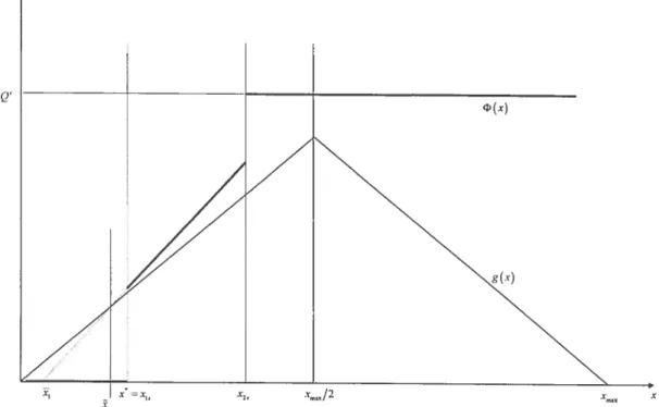
3.11 Steady States when î < _{x15 and g (Xmax/2)}

<Qc.

_{Que $teady $tate}

(Irregular) _$6

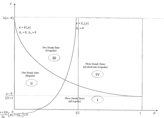
3.12 $teady $tates in the (p, E)-$pace when > 6° $7 3.13 Steady States in the (p,E)-$pace when 6<6° ₈₈

À

_{t’Éternel des Armées, par qui ce rêve devient réa.tité. Merci pour cette grâce!}

À

_{mes défunts parents, Otaire et Martin Lohoues. Que de regrets que vous ne}

puissiez être témoins du parachèvement de cette thèse. Que Dieu vous be’nisse!

À

_{mon épouse, Mar’ie-Michette $onan-Lohoues. Merci pour tout!}

À

_{mes enfants, Éphrain et Nathan Lohoues. Puisse cette thèse constituer pour} vous aussi, une source d ‘inspiration et de motivation pour t ‘avenir.

Je tiens avant tout à remercier et à rendre un vibrant hommage à mon directeur de thèse, Gérard Gaudet, pour sa disponibilité, sa patience et toute sa contribution à la réalisation de ce travail. Il a su orienter et guider mes recherches de manière fructueuse, et surtout m’encourager à ne pas baisser les bras. J’ai beaucoup appris à ses côtés durant toutes ces années de dur labeur.

Je voudrais remercier Rabah Amir, Hassan Benchekroun et Ngo Van Long, ainsi que les participants aux ateliers d’économie des ressources naturelles de Montréal, pour leurs commentaires et suggestions sur différents aspects contenus dans les essais de cette thèse.

J’aimerais remercier le CRDE/CIREQ et le Département de sciences économiques de l’Université de Montréal pour leur soutien financier. Merci aussi à toutes les per sonnes rencontrées au cours de mon cursus de Ph.D. à l’Université de Montréal, notamment le corps professoral, le personnel et les étudiants du département de sciences économiques.

Une partie de cette thèse été rédigée alors que je travaillais à Analysis Group, Inc., où j’ai bénéficié d’un environnement de travail stimulant et flexible qui m’a permis de terminer ce travail. J’aimerais, à ce titre, exprimer toute ma gratitude à Pierre-Yves Crémieux et Marc Van Audenrode pour leur soutien et leurs encoura gements.

Je ne saurais terminer ces propos sans accorder une mention spéciale à ma famille pour son soutien, son amour et sa patience indéfectibles, sans lesquels cette thèse n’aurait jamais abouti. J’adresse donc un vibrant hommage à feu mes parents, Claire et Martin Lohoues, à mon épouse, Marie-Michelle $onan-Lohoues, à mon oncle Roger Lohoues, sans oublier mes frères et soeurs.

INTRODUCTION GÉNÉRALE

Les agents économiques exploitant un stock commun de ressources naturelles ne sont pas nécessairement identiques.

À

titre d’exemple nous pouvons citer le cas d’une industrie de pêche dans laquelle interviennent de grosses multinationales au même titre que de petites entreprises locales ou tout simplement de petits pêcheurs. L’une des caractéristiques de ces multinationales est qu’elles disposent de plus de moyens logistiques et technologiques leur permettant d’avoir un certain avantage quant à la quantité de poissons pêchés, sur les petites entreprises locales et les petits pêcheurs intervenant dans cette industrie. Comme second exemple, nous pouvons aussi citer le cas de l’accès à une nappe aquifère par des intervenants hétérogènes. Parmi eux, l’on pourrait trouver de gra;des multinationales d’embouteillage d’eau minérale ainsi que de petites entreprises locales, dont l’activité est essentiellement à but lucratif.

Dans cette thèse, nous utilisons une approche permettant de prendre en compte cette hétérogénéité. Nous séparons les agents en deux groupes sur la base d’une ca ractéristique intrinsèque permettant de les classer. Nous faisons ainsi l’hypothèse que les agents sont tous identiques au sein d’un même groupe et que le nombre d’agents peut être différent d’un groupe à l’autre. Par cette méthode, nous in troduisons dans nos modèles deux types d’asymétries _{(j) une asymétrie dite «} intrinsèque » qui porte essentiellement sr la caractéristique qui fait la différence entre des agents représentatifs de chaque groupe et (ii) une asymétrie de « taille de groupe » qui concerne la répartition des agents dans chaque groupe. Un des objectifs de cette thèse est justement d’analyser l’impact de ces asymétries sur les équilibres du jeu différentiel résultant de la modélisation de cette situation.

Les jeux différentiels sont des modèles de jeux dynamiques servant à étudier des systèmes évoluant dans le temps, et dont la dynamique peut être décrite par des équations différentielles (Dockner et al. [11]). Ils sont ainsi devenus un outil

privilégié en économie des ressources naturelles, lorsqu’il s’agit de décrire des in teractions stratégiques entre plusieurs agents économiques exploitant une ressource naturelle commune dont l’évolution du stock, qui constitue dans ce cas l’état du système, est décrite par une équation différentielle.

Dans la formalisation des jeux différentiels, deux concepts de solutions sont le plus souvent utilisés t les équilibres de Nash en boucle ouverte (e open-loop Nash equilibria

_»)

_{et les équilibres de Nash en boucle fermée (e closed-loop Nash equi} libria

»)

_{pour lesquels l’attention n’est en général accordée qu’aux équilibres de} Nash markoviens parfaits (e Markov perfect Nash equilibria

»).

Dans le concept des équilibres de Nash en boucle ouverte, la stratégie (dans notre cas, la quantité de ressource extraite par un agent à chaque instant) ne dépend que du temps et de l’état initial du système (le stock initial de la ressource). De ce fait, il s’agit d’un équilibre relativement plus facile à déterminer et servant souvent de référence

(e

benchmark

»)

_{pour des comparaisons à d’autres types d’équilibres (Fudenberg} et Tirole [15]). Cependant, un équilibre avec des stratégies en boucle ouverte, ne sera en général plus un équilibre si pour une quelconque raison, le stock de res source dévie du sentier d’équilibre. Les équilibres de Nash markoviens parfaits sont quant à eux, de par leur construction, des équilibres parfaits en sous-jeux, dont les stratégies dépendent de l’état du système à chaque instant. Ainsi contrairement aux équilibres de Nash en boucle ouverte, les équilibres de Nash markoviens parfaits demeurent des équilibres de Nash même pour des valeurs du stock qui s’écartent du sentier d’équilibre. Cependant, les équilibres de Nash markoviens parfaits, restent plus difficiles à caractériser analytiqilement que les équilibres en boucle ouverte. Pour plus de détails sur les comparaisons entre ces deux types d’équilibres et leurs implications, voir par exemple Reinganum [30], Dockner et al. [10], Clemhout et Wan [7], Dockner et Sorger [12]. et Long et al. [251.

Dans cette thèse, nous nous servons uniquement des équilibres de Nash marko viens parfaits pour caractériser nos équilibres. L’objectif dans ce cas est double

3 non seulement caractériser analytiquement ces équilibres lorsque les asymétries présentées plus haut sont introduites, mais aussi et surtout déterminer les impacts que de telles asymétries pourraient avoir sur les équilibres des jeux différentiels modélisés.

Dans la littérature sur l’exploitation des ressources naturelles communes, dans les jeux différentiels utilisant des équilibres markoviens parfaits, les agents économiques sont généralement considérés comme identiques, souvent pour faciliter la caractérisation de la solution. Des exemples sont, entres autres, Dockner et al. [11] dans lequel les agents se font la concurrence uniquement au cours de l’exploitation de la ressource (l’intrant), et Karp [20] et Mason, Polasky [26] et Benchekroun [1], où les agents se font la concurrence aussi bien pendant l’exploitation, mais aussi au cours de la vente de leur production (Pextrant) sur le marché. Il existe aussi certains modèles qui considèrent des agents hétérogènes présentant un type d’asymétrie, notamment l’asymétrie intrinsèque. En effet, dans leur célèbre modèle formulé en temps discret et connu sous le nom de « f ish War », Levhari et Mirman [21] considèrent deux agents dont la différence se situe a.u niveau de leur taux d’actualisation. Plourde et Yeung [29] proposent une version en temps continue du « Fish War » de Levhari et Mirman, avec plusieurs agents, toujours différant par leurs taux d’actualisation. Ces deux modèles caractérisent leurs équilibres à l’aide de stratégies markoviennes linéaires. Dockuer et $orger [12] considèrent deux agents hétérogènes différant par leur follction d’utilité et caratérisent leurs équilibres à partir de stratégies marko viennes plus complexes. Toutefois, dans aucun de ces modèles à agents hétérogènes, l’effet de la différence entre les agents n’est examiné.

Au mieux de nos connaissances, la prise en compte de l’hétérogénéité entre agents introduisant aussi bien une différence entre les agents (asymétrie intrinsèque), qu’une différence de nombre d’agents dans chaque groupe (asymétrie de taille de groupe) n’a jamais été abordée dans la littérature sur l’exploitation d’une ressource naturelle commune. Ces asymétries pourraient avoir des impacts sur les équilibres

résultant des jeux différentiels considérés. Cette thèse se veut donc une contribution à la littérature à ces deux niveaux. En effet, nous y proposons deux modèles d’agents hétérogènes à asymétrie double, pour lesquels nous caractérisons des équilibres markoviens parfaits et nous analysons l’impact des deux types d’asymétries sur ces équilibres. Dans le premier chapitre, nous déterminons les conditions nécessaires d’utilisation d’une classe particulière de stratégies markoviennes : les stratégies markoviennes linéaires. Dans le second chapitre nous présentons un modèle de « Fish War » avec les deux types d’asymétries et dont l’asymétrie intrinsèque est ca ractérisée par la différence entre les taux d’actualisation des agents. Dans ce second chapitre, les agents se font la concurrence uniquement sur le marché de l’intrant. Ce modèle est amené à vérifier les conditions nécessaires déterminées au premier chapitre pour permettre l’utilisation de stratégies linéaires dans la caractérisation des équilibres. Dans le troisième chapitre nous présentons un modèle dans lequel les agents se font la concurrence aussi bien sur le marché de l’intrant que sur le marché de l’extrant, et qui introduit aussi les deux types d’asymétries. Cette fois, l’asymétrie intrinsèque est saisie à travers la différence entre les coûts marginaux des agents. De façon générale, nous trouvons que les deux types d’asymétries ont des impacts importants sur les stratégies individuelles, sur le taux d’exploitation agrégé et sur les états stationnaires qui découlent des modèles présentés.

De façon plus spécifique, dans le premier chapitre, nous caractérisons les condi tions nécessaires permettant l’utilisation de stratégies markoviennes linéaires dans les jeux différentiels décrivant l’exploitation d’une ressource naturelle commune. De telles stratégies sont par exemple utilisées par Levhari et Mirman [21], Clemhout et Wan [6], Plourde et Yeung [29], Fischer and Mirman [13, 14], Long et Shimo mura [24], et Dockner et al. [11]. Nous montrons que l’existence de tels équilibres est assujettie à l’existence d’une relation précise entre les éléments essentiels du modèle, notamment la fonction d’utilité des agents et la fonction de “dynamique naturelle” ou de reproduction de la ressource exploitée. Ainsi, pour une fonction

5 d’utilité donnée, seule une famille spécifique de fonctions de reproduction est com patible avec l’utilisation de stratégies markoviennes linéaires. De même, lorsque la fonction de reproduction est connue, seule une famille particulière de fonctions d’utilité permet l’utilisation de stratégies linéaires.

Dans le second chapitre, nous étudions un « Fisli War » dans lequel les agents impliqués se font concurrence uniquement sur le marché de l’intrant, c’est-à-dire uniquement au cours de l’exploitation de la ressource, comme c’est le cas notam ment dans Levhari et Mirman [21] et Plourde et Yeung [29] Ces agents sont repartis en deux groupes de tailles potentiellement différentes. Nous examinons l’impact du différentiel de taux d’actualisation (l’asymétrie intrinsèque dans ce cas) et de la répartition des agents (l’asymétrie de taille de groupe) sur l’équilibre de ce jeu. Nous montrons alors qu’au niveau global, des augmentations dans le différentiel de taux d’actualisation et dans la proportion d’agellts avec le taux d’actualisation le plus élevé (les « gros

»),

_{augmentent l’extraction totale et diminuent le stock} de ressource à l’état stationnaire. Cependant, au niveau individuel, l’impact de ces deux types d’asymétrie dépend de la comparaison de l’élasticité de l’utilité mar ginale à l’unité. Pour ce qui est de l’asymétrie de « taille de groupe

»,

lorsque l’élasticité de l’utilité marginale est supérieure (inférieure) à un, une augmentation de la proportion de « gros » agents dans l’industrie, tend à réduire (augmenter) le taux d’extraction des deux types d’agents. Ainsi, chercher à rendre l’industrie plus « homogène » en « gros » agents aura tendance à atténuer (exacerber) la « guerre » engendrée par la concurrence, lorsque l’élasticité de l’utilité marginale est supérieure (inférieure) à un. Concernant l’asymétrie de taux d’actualisation, une augmentation du différentiel augmente toujours le taux d’extraction des « gros » agents. Par contre, pour les « petits » agents, cette augmentation du différentiel de taux d’actualisation tend à réduire (augmenter) leur taux d’extraction lorsque l’élasticité de l’utilité marginale est supérieure (inférieure) à l’unité.

ploitent une ressource naturelle commune et en vendent la production sur le même marché. Dans ce cas et contrairement a.u second chapitre, ces entreprises se font concurrence aussi bien sur le marché de l’intrant que sur le marché de l’extrant, comme cela est le cas dans Benchekroun [1] Deux entreprises représentallt chaque groupe diffèrent l’une de l’autre de par leurs coûts marginaux. Nous avons ainsi un groupe d’entreprises à bas coût marginal auxquelles nous feroit référence en tant que « grosses » entreprises, et un groupe à haut coût marginal que nous présenterons comme étant les « petites » entreprises. Nous caractérisons explici tement les stratégies markoviennes de ce jeu dont le cas symétrique se réduit au modèle de Benchekroun

_[11,

_{ainsi que les effets des deux types d’asymétries sur les} équilibres obtenus. A l’instar de Benchekroun [1], les stratégies d’équilibre que nous trouvons sont caractérisées par trois intervalles de stocks de ressource sur lesquels les entreprises adoptent des comportements différents. En-deçà d’un certain stock seuil, aucune entreprise ne produit. Entre ce stock-seuil et un second stock-seuil, les entreprises exploitent la ressource à des taux linéaires et croissants avec le stock de ressource. Au-delà de ce second stock-seuil, les entreprises exploitent la ressource à des taux constaits et qui correspondent aux taux d’exploitation qu’elles aiiiaient

adoptés si elles se faisaient une concurrence statique à la Courilot. Toutefois, la présence d’asymétries induit des discontinuités dans la stratégie des grosses entre prises, et par conséquent dans le taux d’exploitation agrégé. Nous montrons aussi que le stock-seuil à partir duquel les petites entreprises commencent leur exploita

tion et le stock-seuil à partir duquel elles adoptent leur exploitation à la Cournot statique, sont tous les deux plus élevés lorsque ces entreprises sont en présence de grosses entreprises (cas asymétrique) que lorsqu’elles sont toutes identiques (cas symétrique). Quant aux grosses entreprises, lorsque leur proportion dans l’indus trie dépasse un certain seuil, le stock-seuil auquel elles commencent l’exploitation est plus élevé dans le cas symétrique que dans le cas asymétrique. En-deçà de ce seuil, ces grosses entreprises commencent leur exploitation à un stock-seuil plus bas

z

que dans le cas symétrique. Le stock-seuil auquel elles adoptent leur comportement à la Cournot statique est, quant à lui, toujours plus bas dans le cas asymétrique que dans le cas symétrique où elles sont toutes de grosses entreprises. Nous trou vons aussi que ce modèle admet un ou trois états stationnaires selon la valeur du différentiel de coût marginal (l’asymétrie intrinsèque dans ce cas) ou la répartition des entreprises (l’asymétrie de taille de groupe). Par ailleurs, chacun de ces états stationnaires peut être obtenu en faisant varier les deux types d’asymétries.

ON LIMITS TO THE USE 0F LINEAR MARKOV STRATEGIES IN COMMON PROPERTY NATURAL RESOURCE GAMES

by Gérard Gaudet and Hervé Lohoues’ Abstract

We derive conditions that must be satisfied by the primitives of the problem in order for an equilibrium in linear Ivlarkov strategies to exist in common property natural resource differential games. These conditions impose restrictions on the admissible form of the natural growth function, given a benefit function, or on the admissible form of the benefit function, given a natural growth function.

‘We wish to thank Rabah Amir and Ngo Van Long for their useful comments on an earlier draft.

9 1.1 Introduction

For sorne differential garnes, it can be shownthat there exist equilibrium decision

rules that are linear in the current value of the state variables. These types of strategies, callecl linear Markov strategies, are attractive because of their simplicity and ease of interpretation. They also greatly facilitate the computation of the eqrnlibriurn and of its properties. For these reasons, the analysis is often restricted to this class of equilibria, when they exist. Notable examples in common property resource games are Clemliout and Wan [6], Lehvari and Mirman [21], Plourde and Yeung [29], Fischer and Mirman [13, 14], Long and Shimomura [24] and Dockner

et aÏ. [11].

The use of linear Markov strategies is however lirnited by the restrictions that must be imposed on the primitives of the model in order for such an equilibrium to exist. In this paper, we derive necessary conditions to the use of linear Markov strategies in natural resource differential garnes.

The model is presented in section 1.2. In section 1.3, we derive restrictions that must 5e imposed on the natural growth function, given the frequently assumed constant elasticity utility function. In section 1.1, we clerive restrictions that must be imposed on the utility function, given a specific natural growth function. In section 1.5, we briefly discuss an extension to the case where benefit is derived from the remaining resource stock as well as the flow of consumption. We end with some concluding rernarks in section 1.6.

1.2 The model

Consider a natural resource that is commonly owned and exploited by n eco nomic agents. Denote by x(t) the stock of the resource at time t and by c(t) the rate of harvest of agent i, i = 1. n. If g(r(t)) is the natura.l growth function of the resource stock, then the state variable x(t) evolves according to the differential

equation

±(t) = g(x(t)) - c(t).

(1.1) It is assumed that agent i derives an instantaneous net benefit _{u(c(t)) from his}

harvest, with u’(c1(t)) > 0 and u”(c(t)) <0.

By assumption, we restrict attention to equilibria in stationary linear Markov strategies. Stationary Markov strategies in this context are decision ruies that spe cify an agent’s harvest rate as a function of the current resource stock c(t) =

(x(t)). A linear strategy for agent j is a strategy of the form (x(t)) =

with 6j > 0 a constant.

An equilibrium in linear Markov strategies, if it exists, vil1 necessarily have the property that a best response of agent i to linear strategies being played by each of his n — 1 rivais is also a linear strategy. The question then is What are the minimal restrictions that need to be put on the primitives of the problem (the natural growth function g(x(t)) and the utiiity function u(c)) _{in order for this}

property to be satisfied?

At equilibrium it will he the case that, taking as given tue vector of decision mies j(r)

_j

_{i oflis (n} — 1) rivais, agent i’s ovin decision fuie,

c maxirnizes

f

etu(c)dt (1.2) subject to ±=g(x)—cj—xj (1.3) a#i x(0) = x0 given (1.4) c > 0, lim x(t) > 0, _(1.5) t-.oo

11

where r is agent i’s discount rate.

The current value Harniltonian associated to this problem is

c. = u(c) + j[g(x) — — x j], (1.6)

where X is the shadow value of the resource stock for agent i.

An equilibrium must satisfy, for i = 1 ... ,n, the following set of necessary

conditions, in addition to (1.3) and (1.4)

[‘u’(c) — = 0, u’(c) — À <0, c > 0 (1.7)

= r — g’(x) (1.8)

lim eTt,\ir 0, lim eTt,\i > 0 lim x(t) 0. _(1.9)

t—*00 t—00 t*00

Assume &(x) = jr to be a solution, with > 0. Then, for any x > 0, it wiII be the case that âj = j± auJ hence

(1.10) C

It also follows that (1.3) can be rewritten as =

— — 6i. (1.11)

ii

furthermore, from (1.7) and (1.8), along an interior solution,

= (c) [g’() - -ri] (1.12)

rheie !7(Ci) is the elasticity of marginal utility’, given by

= [ciz)]

(1.13)

‘The reciprocal, 1/i(c), can be interpreted as the instantaneous elasticity of intertemporal substitution.

Therefore, substituting from (1.11) and (1.12) into (1.10), we find that the following condition must be satisfied in order for c = àjx to be a best response

-

H

-

[)

-= 0, (1.14)

\\rhere 5, and the j’s are constants that remain to be determined.

It follows that, for any given utility function u(c), the growth function g(x) must satisfy the following first-order linear differential equation in x

xg’(x) — ij(j)g(x) =

[

j + ri] x —

[

j + jx)x. (1.15) ji ji

Alternatwely, given a growtb function g(Œ), the marginal utility function u’(c) nmst satisfy the following first-order linear differential equation in c

[‘

—

— ciu”ci + [‘(c/) —

—ri] u’(c) = 0. (1.16)

ii ii

1.3 Admissible growth functions, given a utility function

Typicallv, in this type of problem, attention is restricted to the class of utility functions that exhibit a constant elasticity of marginal utility. iDenoting by O > O this elasticity, the utility function may then take the form

u(c) = (1.17)

or

n(c) = 1nc, (1.18)

which is the limiting case of (1.17) for O = 1.2

more general representation of this utility function is u(c) = a(c°)/(1

—

)

+ b or u(c) a mc, + b for O = 1. In the present context, there is no Ioss of generality in setting a = 1 and

In that case, = O, a constant, and (1.15) has as a unique general solution

10+kx° ifO1

g(x) = — (1.19)

(r—&)xln+kr _ifO1,

where k is the constant of integration.

Therefore, given a utility function of the forrn (1.17) or (1.18), a decision rule of the form q5(x) = 6jx wilÏ be a best response to decision rules of the form

j(x) = jx,

j

i, on the part of i’s n

— Ï rivais, only if the growth function is of the forrn

ifO1

g(x) =

(1.20) cix+/3x1nx ifû=1.

Substituting from (1.20) and (1.17) or (1.18) into (1.15), we get the following system of n equations

+ (O— — —(6— 1)c ₌ O if O 1

(1.21) ifO=1

which determines the constant equilibrium values of 6j, i 1, . . . , n. In particular,

with identical agents (i.e., T T, i = 1, .. . ,n), the symmetric equilibrium is given

by T+(O—1) ifO1 nO—(n—1) (1.22) T—B ifO=1.

The class of functions in (1.20) exhibits desirable properties for a natural growth function when the parameter values are restricted to c > 0, /3 < O and O > _{1 (or}

g(ï) = 0, where ₌

(—/)

in the case of 0> 1 (or O <0 _< 1) and = e1

in the case of 0 = i. The stock level collstitutes a stable steady-state iII the absence of harvesting of the resource and captures the idea of the natural carrying capacity of the environment.

A major drawback however is that uuless we restrict the growth function to

= 0, it must. depend explicitly on a parameter of the utility function, namely

0. if the clecision rule

₍₎

= x is to be a best response to j(x) = jx,

j

i.

This also means that unless .8 = O is irnposed. heterogeneity over the O’s is not

admissible, since the grow’th function g(a) must be coinmon to ail agents, by the very nature of the probiem.

1.4 Admissible utility functioiis, given a growth function

Conversely, consider the case where the growth function is known to be of one of the forms iII (1.20), with û, .8 and 0 being known exogenous parameters. Then, frorn (1.16), we have that the elasticity of margillal utility must be given by

o—’

ifg(x)=ûx+/3x°

—cu (ci)

—

t5i

—

u(c) _{f .\} û++ln) —zjii—Ti if g(x) =ûx+j3xlnx. û _{+ 1n}

()

—

—

(1.23)

It follows that a decision mie of the form çj(i) = can be a best response to

decision mies of the form j(x) = f5x,

j $

i, on the part of i’s n

—

1 rivais only if

3lmposing c > 0, /3 < O and O > 1 (or c < 0, _/3 > O and O < (9 < 1) in fact guarantees the sufficiency of conditions (1.7), (1.8) and (1.9). Note that when a = /3 = 0, we have the case of a

15

ij(c) is of the following form A+OBc’ . C + Bc’ if g(x) x + x (1.24) D+E1nc F+E1nc ifg(x)=cx+3x1nx.

Hence the utility function will be of the form

= af e_JZdsdz + b

(1.25) and the marginal utility ftmction of the form

f — fCi -3-1ds u (ci) = ae s _, (1.26) where a > O and ïj(c) _{must be given by (1.24). Strict concavity is assured by} imposing 77(cj) > O in (1.24).

This class of utility functions of course includes as a special case that specified in (1.17) whenever A = OC (with b = O auJ a = 1/(1 O)), or that specified in

(1.18) whenever D F (with b = O auJ a = 1).

Substituting from (1.24) into (1.23), we find that the constant equilibrium so lution for , i = 1,.. . ,n, must satisfy, if g(x) ₌ cx + ,3x°

(i —

o)

—

(o

+ (0 1) — — (O —

fl))

=

o

(1.27) _________ A — — — — and, if g(3;) cx+/3xlnx: (1.28) In particular, with identical agents, the symmetric equilibrium value of will be

gwen, if g(x) = x + /3x°, by

g

(i —

o)

S’° — [n9 — (n — 1)j —r — (9— 1)) = O (1.29) C o—n6 A —(n—1)S—r — and, if g(x) = cx+/3rlnx, by (1.30) Notice that if A = 9C and D F. in which case, as not.ed above,

the utility

function is of the crnstant elasticity form (1.17) and (1.18) respectively, then (1.27) and (1.2$) reduce to (1.21) and (1.29) and (1.30) reduce to (1.22). But the admis sible class of utility functions is wider than the constant elasticity cïass. Again, however, an important drawback is that the parameters of the utility function de-pend explicitly on _{the exogenous pa.rameters of the growth function, namely c,} and O.

1.5 An extension

It is sometimes appropriate to have utility depend not oniy on the ftow of consumption of the resource, _{but also directly on the stock, because of the fiow} of a;nenities it may provide.5 To capture this, assume that agent i derives an instantaneous benefit u(c(t), x(t)) _{from those two sources, with u(c(t), x(t)) > 0,}

u(c(t), x(t)) > 0, u(c(t), x(t)) < O and u1(c(t). x(t)) < 0. Then the equivalent of (1.15) is: xg’(x) — [(6jx, x) —

e(x,

)]g(x) =

[

j +ri] —

[

j + [x, x) —(Sjx, x)]x — S(x,x)x, (1.31)

17 where __ cu(c, x) _{xu(c, x)} — — and (c1,x) ₌

are respectively the elasticity of marginal utility 0f c with respect to c and x aid x)

=

u(àir, x)

is the marginal rate of substitution betweenc and x. Given the function u(c(t), x(t)).

the function g(x) must satisfy the first-order linear differential equation (1.31) if c = 5jc ïs to be a best response.

Consider, as an example, the following version of the constant elasticity utility function, with u> O and O 1 t

u(c,x) _(1.32)

Then j(6jx,x) O, (jX) _{u, $(,x)} = uô/(i — O) and (1.31) has as a general solution t

[ri_ (O—u+ 10)6+(1_O+u)j] _{i_++k° (1.33)}

ii

where k _{is the constant of integration. Hence the growth function lias to be of the}

form t

g(x) _(1.34)

In particular, if u = O, then admissible functions must be of the form

g(x) = x + .

In that case, the utility function is liomogeneous of degree one and hence marginal utility of consumption can be written _{u(c/r, 1), which becomes a constant when}

the Hamiltonian, )(t) must be a constallt. It then follows directly from condition (1.8) tha.t g’(x) _{must be a constant as well. This will be true of any utility fullction} that is homogeneous of degree one in c a.nd r.

The constant equilihrillrn values of j, i = 1 n are obtained as the solution to the following system of n equations

[to

— u) +

1

]

+ (O — u — 1)3 —r — (6—u — 1)ù = 0. (1.35) Setting r = ‘r, the symmetric equilibrium is given by

T+(O—U—l)

- n(O-u)-(n-i)+u/(1-O)

The limiting case of (1.32) for 6 1, u > 0, provides an example of the fact that for g(x) to satisfy condition (1.31), though necessary, is not sufficient for the best response to be linear. The utility function is then given by

‘u(c,x) _{=x°1nc, (1.36)}

and 5x,x) = 1, (ôx,x) = u and S(x,3) = u5[1nx + lncj]. The solution to the cliffèrential equation (1.31) is then

g(x)=

which means that admissible growth functions must be of the form

g(x) = x + x mx +

Substituting for this form of growth function into the differential equation (1.31), wre _{find that it vil1 be satisfiecl only if} j, i = 1, . . . ,n, solves

19

which involves x. Clearly, for agent i’s best response to be linear in x further requires that j — > O, with, in addition, o = [r — na + u ln(—16)]/u. This in turn requires r r for ail i, _{since it is inherent to the problem t.hat the growth}

function is common to ail agents. 1.6 Concluding remarks

The above resuits place in proper perspective models that rely on linear Markov strategies to study the competition over a common property resource, by showing that the parameters of the utility function and of the growth function cannot be chosen independentiy of oe another, but must satisfy a precise relationship. Assi gning specific numerical values to the parameters of functiollal forms that happen to satisfy this relationshxp — for instance a unit elasticity of marginal utility or a linear growth function _{sometimes tends to obscure this fact.}

The papers cited in _{the introduction ail assume specific functional forms for} the utility functioll and the growth function that happen to joilltiy satisfy this necessary relationship. Clemhout and Wan [6] alld Plourde and Yeung [29] both assume a logarithmic utility function as in (1.18) — heilce an elasticity of margillal utihty equal to mie — combined with a growth function as in (1.20) with ₌

1. Lehvari and Mirman [21] assume a discrete time version of the same growth

function, also combined with a logarithmic utility function. This also applies to Fischer and Mirman [13,14], although in those cases the growth functions allow for interaction betweell two _{types of resonirces. Long and Shimomura [24] assume the} utffity function to 5e homogeneous of degree h > O (or the log of such a function). Such a utility firnction exhibits a constant elasticity of 1 — h (or of 1 in the ca.se of the logarithmic version). Their growth function is assumed homogeneous of degree one, which in effect mea.ns a function such as that in (1.20) with = 0. Dockner et aÏ. [11] (chapter 12) study an exemple with a constant elasticity functioll of the form (1.17) alld a growth function as in (1.20) with 1.

GROUP AND SIZE ASYMMETRIES IN A FISH WAR by Hervé Lohoues

Abstract

We present u “fish war” between agents exploiting a common property resource and divided into two groups of potentiafly different sizes. Agents are identical within a group but differ between groups by their discount rates. We examine the impact of discount rate and group size asymmetries

011 the outcornes of the game. ‘Ve show that, ut the industry level, increases in the discount rate

differential and in the proportion of “big” agents (those with the larger discount rate), both increase the aggregate extraction rate and decrease the steady state stock level. However, at the individual level, the impacts depend on whether the elasticity of marginal utility is greater or less than unit;. For the “size” asymmetry, when the elasticity of marginal utility is greater (smaller) than unity, an increase in the proportion of big firms tends to decrease (increase) the individual extraction rates of both types of agents. This means that, making the industry “more hornogeneous” in hig agents vill tend to attenuate the “fish war”, if the elasticity of marginal

utility is greater than one. On the contrary, when the elasticity of marginal utility is Iess than

unity, this will exacerbate the “fish war”. As for the discount rate asymmetry, an increase in the discount rate differential aiways increases the individual extraction rates of the agents with the larger discount rate. However, when the elasticity of marginal utility is greater (smaUer) than unity, this increase in the discount rate differential decreases (increases) the extraction rates of the agents with the srnaller discount rate.

21 2.1 Introduction

Exploitation of a common property resource most often iiwolves agents that are not necessarily identical. They can often be divided into two (or more) groups of different sizes, within which agents are identical. In that case, both intrinsïc differences between representative agents from each group and the size of the groups matter. We will refer to the former as “intrinsic asymmetry” and to the latter as

“size asyrnrnetry”.

In real life, examples of this kind of two-sided asymmetry abound. A first example is the case of fisheries, where it is common to find one or a few “big” multinational fishing firms competing with many “small” local firms, or simply local fishermen exploiting the fishing grounds for subsistence. Another example is the existence of a small number of big water bottiing firrns exploiting an aqiiifer which is also used by many small firms or individuals.

The situations described above can be modelled as a “fish war”, first develo ped in the seminal paper by Levhari and Mirman [21] to describe the economic implications inherent to fishing confticts. In a larger sense, this analysis can be ex tended to any other duopolistic and oligopolistic situation in which maiiy players have access to the same replenishable (or exhaustible) natural resource stock ow

ned in common. In the literature, this is referred to as a common property resource exploitation game. As a differential game, this model has two basic features. Tire first concerns tire strategic aspect : each of the players wiÏl take into account tire actions of the other participants. Tire second concerns tire dynarnics of the resource stock _{the future size or rate of growth is affected by the actions undertaken by} the players.

We will assume tire industry to be composed of two types of agents differing by their discount rates. A first type exhihits a high discount rate and the other type, a iow discount rate. We will refer to these agents as the “big” agents and “small”

agents respectively. To take the example of the fisheries, we can assume that the big multinational firrns have access to alternative investment opportunities that

have a higher rate of return. They use this rate of return to discount the yields over time of their fishing activities. Conversely, the srnall local fishermen have a low rate of return on alternative iuvestments.

We wilÏ restrict attention to equilibria in stationary linear l\/Iarkov strategies. A I\4arkov perfect Nash equilibrium (MPNE) is an equilibrium of a dynamic game in whïch players adopt decision rules that are contingent upon the current state of the game. MPNEs can he tedious to derive explicitly and are therefore often restricted to those in which decision rules are linear in the current value of the state variable, if such equilibria exist. Linear strategies greatly facilitate the computation of the equilibrium and of its properties and have been used by a number of authors to deal with common property resource games.’

Our model is closely related to those of Levhari and i\’Iirman [211 and Plourde and Yeung [29]. Levhari auJ Mirman assume there are two players and use a re cursive dynamic Cournot-Nash approach to solve their duopolistic discrete time dynamic game. Plourde and Yeung present a continuous time version of the Lev han and Mirman’s model with n players. In both models, the agents differ from one another by their discount rates. This means that these models examine only a one-sided asymmetry, corresponding to what we cali here the “intninsic” asym metry. Our model also includes this “intninsic” asymmetry betweeu the two types of agents, who differ in their discount rates. In addition, we introduce a poten tial “size” asymmetry by assuming that the number of each of the two types of agents may differ. Our aim is to examine how these two types of asymmetries affect the outcomes of the game. IViore precisely, we address the impact of the discount

‘See for instance, Clemhout and Wan [6], Lehvari and Mirman [21], Plourde and Yeung [29], Fischer and Mirman [13, 14], Long and Shirnomura [24] and Dockner et aÏ. [11]. Gaudet and Lohoues [16] establish necessary conditions for the use of such strategies.

23 rate differential alld the impact of an increase iII the proportion of big agents on

the individual and aggregate equilibrium extraction rates and on the steady state resource stock level, when it exists.

We show that both the size and intrinsic asymmetries do affect the equilibrium indiviclual anci aggregate strategies. At the industry level, increases in the propor tion of big agents and in the discount rate differential, both illcrease the aggregate extraction rate and decrease the steady state stock. However, at the individual level, the impact depends on the asymmetry examined and on whether the elasti city of marginal utiÏity is greater or less than ullity. It will be shown that, for the size asymmetry, when the elasticity of marginal utility is greater (smaller) than

unity, _{an increase in the proportion of hig firms tellds to decrease (increase) the} individual extraction rates of both types of players. This means that, making the industry “more homogeneous” in _{big agents will tend to attenuate the “fish war”} when _{the elasticity of marginal utility is greater than ope. 011 the contrary, when} the elasticity or marginal utility is less than ullity, this will exacerbate the “fish

war”. As _{for the intrinsic asymmetry, an increase in the discount rate differential} aiways increases the individual extraction rates of the big agents. However, when the elasticity of marginal utility is greater (srnaller) than unity, an increase in the discount rate differential tends to decrease (increase) the extraction rates of the srnall agents.

The remainder of _{the paper is organized as follows. The model is presented} and solveci in section 2.2. In section 2.3, we analyze how both types of asymmetries affect the equilibrium outcornes of the gaine. We conclude bysumming up our main findings in section 2.4.

2.2 The model

Consider a natural resource that is commonly owned and exploited by n econo mic agents divided into two groups a group of n “big” agents and a group of n,

“small” agents. They are identical within a group but asymmetric between groups. A representative member from a given group k, k = s, b ha.s a discount rate _r.

We assume that Tb r8, that is the big agents have larger discount rate than the

srnall agents. The agents compete by _{choosing the extraction rates that maximize} the present value of their flows of discounted benefits.

Denote by x(t) the stock of the resource at time t and byc(t) _{the rate ofharvest} of a given agent i, i = 1,, . . ,n. We assume that agent i clerives

an instantaneous net benefit u(c(t)) _{from lis harvest, with u(c) Seing of the form}

n(c) = + b.

(2.1) where O is a strictly positive constant such that 8 1, a O, alld b a positive

constant. The limiting case of O = 1 is u(c) = aluc + b.2 The specification _in

(2.1) gives an isoelastic utility function, very often used in econornics, for which the elasticity of marginal utility is given by îi(c) = —cu”(c)/u’(c) ₌

o.

_{We have}

that u’(c) > O and u”(c) < O, that is ‘u(.) _{is an increasing anci strictly concave} function of the extraction rate. We will hereafter, without loss of generality, assume

a=1.

The natural growth function of the resource is taken to 5e of the following forrn:

g() = —f3x°,

(2.2) where assumptions on parameters u, a’ and _{will 5e made such that g(x) is} concave.4.

2rfhjs is the utility function used by Plourde and Yeung _{[291 and Levhari and Mirman [21]} with b = O.

3The reciprocal, 1/i(c) = 1/6, can be interpreted as the instantaneous elasticity of intertem poral substitution.

4The function g(z) is concave either with o 1 and a _{3 O or with u 1 ancl n O.}

It is important however that n and _{not differ in sign, in order for the maximum sustainable} yield, given by g’(xMsy) _{O, and the ca.rrying capacity, given by g (K)}

O, K O, both exist. and be positive.

25

By assumption, we restrict attention t.o equilibria in stationary linear Ma.rkov strategies. $tationary Markov strategies in this context are decision rues that spe cify an agerit’s harvest rate as a function of the current resource stock _c(t) = j(x(t)). _{A linear strategy for agent i is a strategy of the forrn (x(t)) =}

where j > _{O is a constant that represents the harvesting effort of agent} i. In that case, taking as given the vector of decision rules j()

= jx,

j

j of his (n — 1) rivais, agent i’s own clecision rule, c = (x), maxirnizes

j

e’u(c)dt _(2.3) subject to (2.4) y z xo given _(2.5) c > _O, lim x(t) > _{0. (2.6)}

The current value Hamiltonian associateci to this problem is

H(x, c, j) = u(c) + À[g(x) — c — , (2.7)

i$i

where À, is the shadow value of the resource stock for agent i.

An eciuilibriurn must satisfv, for i = 1 n, the foilowing set of necessary conditions, in addition to (2.4) and (2.5)

[u’(c) — )]c = O, n’(c)

— Àj < O , c > 0 (2.8) (2.9) lim ertÀx _{O, 11m eÀ > 0. lim x(t)}

0. (2.10)

t-+œ

guarantees that the necessary conditions are also sufficient.

Assume j() = 6j3 to 5e a solution. Then, for any x > O, it will be the case that éj j± and hence

(2.11)

c X

It also follows that (2.4) can 5e rewritten as

(2.12)

32

Furthermore, from (2.8) and (2.9). along an interior solution,

=

H

[91(X)

--

].

(2.13)

Therefore, substituting from (2.12) and (2.13) into (2.11), we find that the following condition must be satisfied in order for c = 5r to 5e a best response

[‘()

— — — = 0, (2.14) ii ii

where j and the j’s are constants tÏiat remain to 5e determinecl.

With the specifications iII (2.1) and (2.2), this last condition simplifies to

—(1— O)Y —T + (1— O)c —L(a—O)x’ = 0. (2.15)

ji

In order for the hest respose of agent j to 5e linear, and hence the c’s to 5e constant. we _{must therefore impose a.t least one of the following three restrictions}

u = 0 or B = O or u = 1. _(2.16) Under one or the other of those assumptions, condition (2.15) becomes

0 —(1— = r —(1— 0)2’ _(2.17)

27 where

t

_{ifeithera=0or=O}

(2.18)

t

‘ o=1

Now let us 5e more specific about the conditions in (2.16) which _{deal with} conditions for the use of linear strategies in our model. If o- = O (a1d then

there exists a specific relationship between the utility function of the agents _and the growth function of the resource. In such a case, when O > 1, the condition

for concavity of g(x) (see footuote 4) implies that c > > _{0. When O < 1, we}

must have < <

0. In addition, in the case where strict concavity of the growth

function is required, e.g. for the existence of a steady state, we must have _0. If u _{O (and then y} = a

—

),

it is necessary that either ₌ O or u

= 1

in order t.o ensure the existence of an equilibrium with linear strategies. _{In other} words, if u _{O, the growth function must necessarily be linear in order for the 5’s} to be constant. When the growth function is linear, there exists no steady state.

The constants 5’s are determined by solving the system of equations in (2.17) which, when taking into account the fact that there are two types of agents, can 5e rewritten in the following matrix form

1 (1 —0)n3 _{—(1 —O)flb —(1—0)7}

(2.19) —(1—O)n3 _{1—(1—O)flb}

Tb-(1O)7

the solutions to which are

5 — —(1 —O)[7— (rb —r8)nbj (990) 1—(1—O)(n8+nb) and 5rb(10)[7+(rbr3)fl8] (291) Finally, the expression of the equilibrium individual extraction rate foi’ a represen

tative agent of a given group k = s, b, k 1, Ï = s, b is

C = k(X)

[

_)7t]]

. (2.22)

At the industry level, the equilibrium aggregate extraction rate is given by = n3(x) + _{flb(X) =}

where _{is the aggregate harvesting effort t}

— [r — (1 — 0)7] (Rs +

flb) + (rb — r) b

(2 23) 1—(1—O)(n5+nb)

We will assume that, the parameters of the problem and the numbers of agents are such that the extraction efforts are strictly positive.

These strategies eau be used to derive the dynamic behavior of the resource stock. In particular, the steady state stock level, when it exists,5 is giveil by

— (n8 + flb) Ts — (rb — r8)b

(224) [1- (1-0) (n +flb)]

for identical agents, that is, whell Tb r8, the individual harvesting efforts are

identical and equal to r — (Ï — 0)7

1—(1—0)n (2.25)

and the industry harvesting effort is [r—(1—0)7]n

9

1—(1—0)n .

(2.6)

5A finite steady state exists only in the case where ci = _{6 andg(x) is strictly concave. that is, in}

addition to the conditions in footnote 4, we must also have O,u O and u 1. Moreover, for

O < _{1, it must be verified that u > r.}

These assumptions ensure that the non-coopera.tive solution implies convergence of the resource st.ock to a strictly positive steady state level .

29 The symmetric case steady state stock level, whell it exists, is

c—rir X

[1—(1—O)n] (2.27)

2.3 Effects of the asymmetries

Notice from (2.20) _{and (2.21) t.hat the difference in the individual harvesting} efforts is exactly equal to the differential in the discount rates, no matter the value of _{and no matter the number of agents. In particular}

— ₌

— r 0.

(2.28) That is, the more important the discount rate asyrnmetry, the larger the effort differential. This also means that agents with higher discount rates will harvest at higher rates.

We now turn to the analysis of equations (2.20), (2.21), (2.23) and (2.24) to examine how both discount rate and size asymmetries affect the players’ strategies and the resource dynamics at equilibrium. To do this, let e = — r and p ₌ be respectively the discount rate differential and t.he proportion of big agents in the illdustry. For the sake of the discussion, normalize the total number of firrns to one (n = 1). Then, (2.20), (2.21), (2.23) and (2.24) becorne respectively

229 o rb—(l—o)[7+(1—p)e] 230 A r5—(1—O)7+pe (2.31) and (2.32)

2.3.1 _{Impacts of “size” asymmetry}

Consider first the impacts of the “size” asymmetry. Differentiating (2.29) to (2.32) with respect to p, we get

— ab — (1 — 2 33

t.)

8L 1 = 0, (2.34) and <0. _(2.35)

The sign of the derivatives in (2.33) oniy depend on whether O is greater or smalier than one. However the sign of the derivative in (2.34) is aiways positive and does not depend 011 that comparison. Aiso, when the steady state exists (see

footnote 5 and comments n conditions (2.16)), (1 — O) and /3 are aiways of opposite signs. Therefore, the sign of the derivative in (2.35) is aiways negative. Notice that the signs of parameters c and

_/3

_{do not matter in the determination of the signs of} these derivatives, only the sign of (1 — O) leads the resuÏts.

At the industry level, equations (2.34) and (2.35) suggest that an increase in the relative number of big agents increases the total amount of resource extracted and decreases the steady state resorce stock, no matter the value of O. This means that making the industry more homogeneous in big agents is “resource consuming”, whereas making it more hornogeneous in small agents (decreasing p) conserves the resource.

At the inclividual level, equation (2.33) shows tliat the impact of the size asym metry is the saine for ail the agents no matter their type and depends on whether O is greater or less than one. When the elasticity of_{marginal utility exceeds unity, an} increase in the relative size of the group of big firms tends to reduce the individual extraction rates of both types of piayers, resulting in a attenuation of the “fish