Phase I : Feasibility study at laboratory level
Final report
Fondation Universitaire Luxembourgeoise
Arlon – Belgium
Jacques NICOLAS
Jindriska MATERNOVA
Anne-Claude ROMAIN
Véronique WIERTZ
December 1998
General objective
The ultimate goal of the project is the development of a mobile compound composition tester, able to be used in the field (e.g. on retread tyre).
Goodyear entrusted F.U.L. with a first six months task, with the limited aim of studying the feasibility of a detection principle at the laboratory level.
The compound composition tester that F.U.L. intends to develop is based on the local heating of the compound (either pyrolysis or combustion), generating a gaseous emission. This emission is typical of the compound composition and can be identified by a suitable system consisting in a gas sensor array and a discrimination software tool.
The first phase (6 months) consists in a feasibility study, at laboratory level, of the identification principle. It is considered that this limited goal is reached when the system is able to discriminate, with acceptable repeatability, three tire compositions : natural rubber (NR), polybutadiene (PBD) and styrene-butadiene copolymer with 23 % styrene (SBR), and, possibly, mixtures NR-PBD, NR-SBR, PBD-SBR.
Those tests are made on "clean" samples supplied by Goodyear.
It is important to notice that this feasibility study is held at the laboratory level on a specific testing bench, whose size and operational conditions are not adapted to field working yet.
In the case of success of this first phase, the partners may decide upon continuation of the research to a subsequent phase towards the development of a mobile tester prototype.
It is obvious that, during this possible second phase, a much more simple solution should be considered, with lighter devices and autonomous microprocessor-driven control board.
Material and methods
Compound samples
Goodyear supplied us with 7 types of compound samples (80 80 5 mm), with 7 various polymer compositions (table 1) :
Compound # Polymer composition
144601 100% Natural Rubber (polyisoprene) (NR)
144604 100% Styrene-Butadiene copolymer (23% Styrene) (SBR) 144607 100% Polybutadiene (PBD)
144610 mixture NR:PBD 70:30
144613 mixture SBR:PBD 70:30
144616 mixture NR:SBR 70:30
144619 mixture SBR:PBD 70:30 different Carbon black level (SBR+PBD/C)
Table 1 : Polymer composition of the Goodyear compounds given to FUL
Gas preparation assembly
Definitions
Combustion is a chemical reaction in which a substance combines with oxygen, producing heat and eventually
light and flame.
Pyrolysis is a chemical decomposition of a material by the action of heat in oxygen-free condition (without the
Assembly
Without prejudging the best solution for the heat treatment of the compound samples (either pyrolysis or combustion, or something between), the tests are carried out in an one-liter box either under nitrogen flow, or under air flow, with the help of a laser diode.
The box is made in Perspex®. During the feasibility step of the project, and for the whole assembly, we decided indeed to work as far as possible with transparent material, in order to visualize phenomena (smoke aspect, direction of flow, laser impact on the sample, …).
The box is a 10x10x10 cm cube. The inlet of the laser beam is a 1 cm split grooved in the middle of the front side and surrounded by a soft Teflon® gasket to reduce gas leakage through that opening (later, a glass sheet has been placed on the split to reduce excessive leakage).
On lateral sides, two opposite fittings allow the flow of incoming carrier gas and exhaust gas mixture respectively (see figure 1).
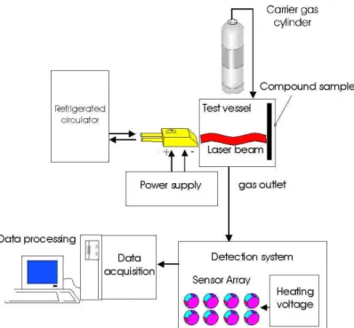
Figure 1 : Gas generation assembly
The compound sample is a 80x80x5 mm slice. It is placed on a metallic surface and it is held laterally by two aluminum strips. After sliding the whole sample holder assembly against the back side of the box, an airtight cover is placed and screwed on the top.
With that device, the laser beam path is about 9 cm long from the diode to the impact on the compound sample.
Laser diode
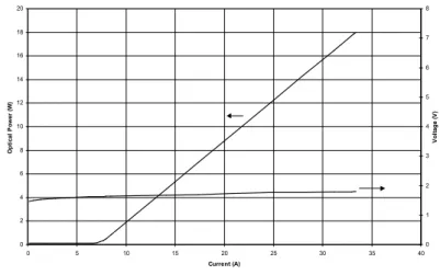
The laser beam is generated by an array of laser diodes : model TH-C1417-P0 from Thomson-CSF. It emits a beam in the near infrared, at 807.1 nm (figure 2).
0 2 4 6 8 10 12 14 16 18 20 0 5 10 15 20 25 30 35 40 Current (A) O p ti ca l P o w er ( W ) 0 1 2 3 4 5 6 7 8 V o lt ag e (V )
Figure 2 : Laser diode characterisics
The device is used at 13 A, 1.65 V (optical power of the beam 4 Watts) for first test and at 18 A, 1.75 V (optical power of the beam 7.5 Watts) for further tests.
The power is supplied by an ELECTRO-AUTOMATIK instrument, current or voltage limited, in the range 0… 16 V and 0…40 A.
In order to maintain the diode at about 20°C, or below, the heat is drained by water through plastic pipes coupled to two suitable fittings on the diode. The circuit closes in a refrigerated circulator (RTE-200D from NESLAB), designed to provide temperature control. The unit consists in a circulation pump, stainless steel reservoir (6 liters) and a temperature controller.
Photo 1 shows the gas generation test box.
Photo 1 : View of the gas generation test box.
Sensor array
Different types
Many gas sensors capable of detecting the components of the gas mixture are commercially available : metallic oxides
MOSFET's
conducting polymers quartz microbalances surface acoustic waves pellistors
electrochemical sensors thermal conductivity sensors
The experiments are carried out with metallic oxide sensors (either thick film technology or thin film technology) and with MOSFET's.
Metallic oxide sensor – thick film technology
For the metallic oxide sensors with thick film technology, we chose to work with discrete components from the Japanese manufacturer FIGARO.
Table 2 shows the 8 sensors chosen for the application.
Reference number Recommended application
TGS842 Methane
TGS822 Organic solvent vapors
TGS813 Combustible gas
TGS800 Air contaminants
TGS824 Toxic gases and ammonia
TGS825 Hydrogen sulfide
TGS2180 Water vapor
TGS2610 Combustible gases
Table 2 : Eight FIGARO sensors chosen for the feasibility study, with the application recommended by the manufacturer.
The sensing material in TGS gas sensors is metal oxide, most typically SnO2. When a metal oxide crystal, such
as SnO2, is heated at a certain high temperature (300 … 350 °C) in air, oxygen is adsorbed on the crystal surface
with a negative charge, with a net effect of generating an electrical resistance in the sensor.
In the presence of a deoxidizing gas, the surface density of the negatively charged oxygen decreases, so the sensor resistance decreases.
The relationship between the sensor resistance and the concentration of deoxidizing gas can be expressed by the following equation over a certain range of gas concentration :
where
R = electrical resistance of the sensor A, = constants
[C] = gas concentration
Sensor selectivity is improved by the addition of some catalyst materials (Pt, Pd, …), allowing the manufacturer to propose some recommended applications (see table 2). However, any sensor may reacts to any deoxidizing gas. This first feasibility step considers thus a 8-sensor array : the obtained results could show that only some of these sensors could be retain for further prototyping, according to their particular sensitivity to the compound composition.
TGS sensors are designed to show optimum sensitivity characteristics under a certain constant heater voltage, around 5 V. A single 5 V power supply is used to heat the eight sensors in parallel, consuming a total current of about 1 A.
The eight sensors are mounted on an electronic board (Eurocard 160x100 mm format). A 10-contact screw terminal allows the connection to the heating power supply and a 50-pin flat cable connector is compatible with the data acquisition board.
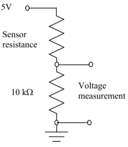
The signal output is obtained through 10 k load resistors in series with the sensor resistor (figure 3).
Figure 3 : Potentiometer assembly chosen for the application.
In a first design, the 5V voltage was supplied by the acquisition board, but we have noted that the signal stability was improved when the reference voltage for the sensor measurement was provided by the power supply already used for the sensors heating.
Metallic oxide sensor – thin film technology
In the final design of the mobile instrument, we should use compact sensor array with suitable miniaturized electronics. That is the reason why we visited the Swiss sensor manufacturer MICROSENS s.a. on May, 29th
1998 and why a complete MICROSENS measuring system, with associated software was purchased, together with 5 sensor-array prototypes.
The multisensors series form Microsens is based on thin-film, metal-oxide technology. Thin-film metal-oxide technology is important for its compatibility with the high precision of semiconductor manufacturing processes. This compatibility ensures reproducible, reliable, and economical sensors and enables the integration of the sensor with sophisticated functions such as signal conditioning, self-calibration, and communication. The multisensor series features an embedded heater layer to raise the temperature of the metal-oxide film to be sensitive to the target gas and micromachined silicon diaphragm for reduced power consumption.
Microsens offers customized batch manufacturing of integrated sensors. There are no standard product : sensor specifications are defined by the user. The multisensors differ either by the sensitive layer (either SnO2, doped
with palladium or platinum, or Nb2O5), or by the electrode geometry (either standard, or interdigited = lower
distance between electrodes). They are packaged in standard TO8 metal can (12 pins) and each package contains either 4 or 6 sensors.
Table 3 shows the characteristics of the 5 multisensors provided by Microsens.
The sensor selectivity is ensured by the type of sensitive layer or by the type of electrode geometry, but also by the operational conditions : heating temperature level (generally between 100 and 500°C) and heating sequence (continuous, step, triangle, pulse).
5V Sensor resistance
Multisensor
identification Number ofsensors Sensitive layer Electrode geometry
14A08 4 1 and 3 SnO2 undoped
2 and 4 SnO2 Pd-doped
standard
1AE 4 1 : SnO2 undoped
2 : Nb2O5
3 : SnO2 Pd-doped
4 : SnO2 Pt-doped
standard
14D19 6 undoped SnO2 1, 2 and 3 : standard
4, 5 and 6 : interdigited
01D28 6 SnO2 Pd-doped 1, 2 and 3 : standard
4, 5 and 6 : interdigited
1CEC5527 6 1, 3 and 4 : SnO2 undoped
2 : SnO2 – Pd-doped
4 : SnO2 – Pt doped
6 : Nb2O5
standard
Table 3 : Characteristics of the 5 multisensors supplied by Microsens
In order to test the various possibilities, we have purchased by Microsens a multisensor evaluation electronic board, able to manage up to 6 sensors in the same chip : both heating (temperature level and heating sequence) and signal recording are provided by that board. It can be connected to a computer through the standard RS232 serial line and a software is also supplied to drive the evaluation board.
Unlike the TGS sensors, the Microsens multisensors aren't recommended for given classes of applications. The user must test himself the multisensors, choosing the right sensitive layer and electrode geometry for his specific application, as well as fitting the heating conditions for best sensitivity and selectivity.
For each multisensor, there are more than 100 possible combinations, and we got 5 multisensors !
It is almost impossible to test systematically all the sensors in all the possible combinations. For this feasibility study, we tested only one sensor (the 14A08) with very simple operational conditions. If that test gives already good results, a more optimal choice will give still better results : it should be sought in further research phases. The TO8 package containing the 4 or 6 sensor-array is plugged into a Teflon socket at one end of a cable, the other end being connected to the evaluation board through a DB25 connector.
MOSFET's
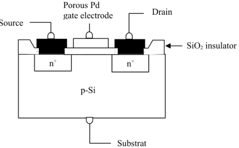
Figure 4 shows the structure of a MOSFET in which the gate is made of a gas-sensitive metal, e.g. palladium.
Figure 4 : Structure of a Pd gate gas-sensitive MOSFET
n+ n+ p-Si Substrat Source Drain SiO2 insulator Porous Pd gate electrode
These microsensors, first proposed by Lundström in 1975, like familiar MOSFET's, exhibit a threshold voltage VT between source and gate for which a current passes between source and drain. But the gas sensible
MOSFET's show a shift VT which depends upon the gas concentration.
These devices are particularly sensitive to hydrogen down to the ppm level. The use of other gate materials (Ir, Pt, …) and of different operation temperatures has led to reasonable specificity to gases such as NH3, H2S and
ethanol. However, the commercial success of the MOSFET chemotransistor has been limited through their poor stability when compared to other metallic oxide gas sensors.
We have tested MOSFET's only during one-off experiment with the commercial e-nose from the Swedish manufacturer NST (see below).
Gas flow
The recommended operation with metallic oxide-based sensors is : firstly creating the "base line" with a reference gas, usually, clean and dry air;
secondly laying the test gas gently flow onto the sensor and measuring the sensor resistance after stabilization.
The effective signal is the relative difference of the sensor resistance values respectively with reference air and with test gas.
For our testing bench, we chose to "clean" the sensors by a static contact with the laboratory air : after a measurement, the recovery time before reaching the base line back is about 15 minutes.
However, in order to avoid sensor reaction delay, dynamic operation is chosen for the measurement itself, with direct flow of a carrier gas onto the sensor (at very low flow rate).
Thus, the sensor signal can be characterized either by the static contact with the air of the laboratory (base line), or by the dynamic flow of the carrier gas (nitrogen or air), before heat treatment, or finally by the dynamic flow of the carrier gas loaded with the vapor generated by the laser beam onto the compound during the heat treatment.
For piping and connectors, as well as for boxes and supports, we try to use neutral materials to avoid gas adsorption on the surfaces (Perspex®, Tygon®, …).
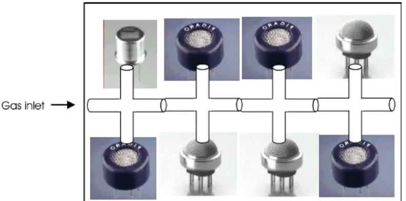
For TGS sensors, the carrier gas passes through 4 cross connectors placed in series (figure 5).
Figure 5 : The array of 8-TGS sensors and the fittings used for gas flow
Photo 2 : Electronic board with the 8 sensors array and gas fittings
For the Microsens multisensor, the end of the cable, with the chip plugged into a socket, is simply inserted in a small cast aluminum box (45 x 40 x 25 mm), as shown in photo 3.
Photo 3 : Small cast aluminum box used as sensor chamber for the Microsens multisensor (the box is open to see the sensor)
In the NST 3220 Lab Emission Analyzer, the reference air is supplied by a gas bottle or alternatively, the air of the laboratory is pumped through suitable filter. The sample gas is allowed to flow into the sensor chamber through a needle and at regulated flow rate of 5 to 150 ml/min. The NST 3220 employs an advanced gas sensor array with 10 NST MOSFET sensors and 5 MOS sensors.
Of course, a commercial instrument should give better results than experimental assemblies. It is well known that commercial e-nose give always good results if the gas sensor array, the operational procedure, and the pattern recognition mathematical tool are sufficiently optimized (to the detriment of simplicity). If we just wish to prove that the e-nose technology is adapted to the recognition of the vapor generated around the tire compounds, we have simply to buy a commercial electronic nose ("e-nose"), and to test samples coming from our laser chamber. But the aim is somewhat different in the context of this feasibility study : the final goal is to design a prototype of mobile instrument, easy to handle, able to work in the workshop conditions and with results easily understood by the operator. So, although the design of the mobile instrument is beyond the scope of the actual first phase, we try to carry out the tests with operational conditions close to the workshop ones : sensor chamber as "open" as possible, avoiding as far as possible clean reference air and strict flow rate control for the inlet gas.
It is expected, even before the measurements, that the results obtained with such material and conditions should be worse than those obtained with "true" laboratory analyzers. But if we nevertheless achieve a good classification with our experimental devices, we could conclude at the feasibility of the compound composition tester.
Data acquisition
For the TGS sensors, data acquisition is performed with the help of a National Instruments AT-MOI-16XE-50 plug-and-play board for the PC-AT and compatible computers. This board features 16-bit analog to digital converter with 16 single-ended or 8 differential analog inputs. Input signals ranges are software selectable between ±0.1 V and ±10 V either bipolar or unipolar.
We use 8 single-ended analog inputs.
The data acquisition board is driven by LabView, a program development software package designed for data acquisition and control applications. It features interactive graphics, a state-of-the-art user interface, extensive libraries and a powerful graphical programming language.
The whole system makes up a high performance assembly, allowing versatile operation, which is essential for this first feasibility study (figure 6).
Figure 6 : Whole testing bench drawn up for the feasibility study.
For the test of Microsens multisensors, the "data acquisition" and "heating voltage" boards of figure 6 are replaced by the evaluation board and the "LabView" software is replaced by a specific computer code supplied by Microsens.
For the operation with the NST Emission Analyzer, the gas produced by heat treatment ("gas outlet" of figure 6) is sampled in Tedlar bags and presented to the NST electronic nose, located in an other room.
General considerations
Classification methods are used with the aim of discriminating the odor origin (NR, PBD, SBR, or mixtures, ...) on the basis of concentrations of a limited number of sensors signals. Two kinds of methods may be used : either unsupervised procedures, or supervised procedures.
Unsupervised procedures are free to respond to input data and to build up a "model" which is able to cluster the observations into some groups showing similar behavior with regard to the observed variables. Rules or models derived like this should possibly serve to allocate new observations to one of the set of defined classes. Nevertheless, the aim of those procedures is chiefly to bring out patterns of similarities or typical differences among observations, not to allocate them. Such methods are qualified as exploratory methods, since they are mostly used to achieve a description of relationships and associations amongst the variables or amongst the observations.
On the contrary, supervised techniques have a teacher providing target groups, besides the input stimuli. Each such procedure has as its basis, a series of variables, here corresponding for example to the eight signals from the sensor array whose membership in a specific group (e.g. NR, SBR or PBD) is well known.
A new item is then diagnosed by determining how typical its individual pattern of variables is of a given group. So, that new item can be assigned to that group.
For each procedures type, we should use either statistical methods or neural networks methods.
Statistical methods belong to the so-called "multivariate analyses", able to handle many variables, sometimes nearly as numerous as the observations. They are generally based on the correlation matrix between the variables under investigation or on the concept of distance between observations : those lying close to another one being placed in the same group. They involve also a graphical layout allowing to identify the different groups by a simple visual examination.
Neural networks are composed of many simple elements operating in parallel. These elements are inspired by biological nervous systems. The network function is determined largely by the connections between elements. With artificial neural networks (ANNs), it is not necessary to obtain an explicit representation of a solution but rather let the network come up with its own implicit representation.
Representation of problems with ANNs may be qualified as "parallel", i.e. information processing takes place in
many neurons at the same time, and "distributed", i.e. there is no central memory, but that representation is stored in the connections between the neurons.
Statistical methods
Principal components analysis (PCA) aims to achieve a parsimonious description of the problem, that means
essentially reducing the number of variables whilst preserving as much of the original information as possible. To reach this latter goal, rather than simply choosing a subset of the original variables, PCA constructs a number of new variables (the principal components) which are linear combinations of the original. The coefficients of these linear combinations are chosen so that the new variables are uncorrelated and, in addition, are such that the first few of them retain most of the information included in the original variables. This procedure allows often to only retain the first two principal components and to represent in a X-Y plot both the original variables and the scores of each observation, as individual points in the X-Y plane. A small distance between two such points means that the two variables or the two observations or the variable and the observation are linked together.
Cluster analysis aims at the classification of the observations based on similarities and differences among them.
Identifying such groups involves an assessment of relative distances between the points. An Euclidean distance may be used, but in some instance, measures of "similarity" between pairs of observations rather than distances are calculated.
Finally, discriminant analysis may be defined as an assignment technique using a priori knowledge of groups of observations. The goal is to construct some discriminant functions, which are linear combinations of the original variables, and which can be used to discriminate the different classes. So, further observations, for which the group membership is unknown, may be classified easily.
Discriminant analysis is the one that is particularly used in the frame of this report to illustrate the classification results.
Neural networks
A neuron is simply an elementary block receiving inputs from other neurons or from input data. The connections between neurons are realised by adaptive synapses which are weights with positive or negative values.
The artificial neuron "fires" (represented by an output 1) if the weighted sum of its inputs exceeds some threshold value. If this sum lies below the threshold, the output is zero.
The mathematical transfer function of the neuron is thus simply a hard limit function exhibiting either 0 or 1. Generally, a more complex neuron is used : the log-sigmoid one, which is a more "continuous" version of the former, but the principle is the same.
The neural network is generally made up of an input interface connected to input data, of an output layer of neurons giving the problem "solutions" at their outputs and of one or more intermediate hidden layers of neurons. Pattern classification task is achieved by presenting a specific input pattern (specific values of a set of variables, here the sensors signals) to the network while simultaneously showing the "solution", i.e. the class information (NR, SBR, PBD, …) , to its outputs. All the weight values and the threshold values for all the neurons in the network adjust themselves in order to give the right response to the input vector.
Training the network consists in presenting several times all the available input vectors (i.e. all observations) to the network in order to update weights and thresholds until process convergence.
At this time, any input may be presented to the network and it will respond with the correct output target vector. If an observation not belonging to the training set is presented to the network, the network will respond with an output (a classification) similar to that exhibited for input observations close to this new one.
The learning rule mostly used by FUL is the "backpropagation" algorithm and is a supervised algorithm.
In the frame of the present study, for the test with our own detectors, we used off-line data processing, either with STATISTICA (for statistical methods) or with MATLAB (for ANN). For the tests with the NST instrument, we used the computer program driving the analyzer which is also able to process the data.
Results
Physico-Chemical Analysis
Firstly, some GC-MS analyses are carried out in order to give preliminary ideas of the main components present in each tire compounds.
Gas volumes generated by the heat treatment are sampled in charcoal cartridges (type ORBO 32S) at a flowrate of 100 ml/min during 15 minutes, either under nitrogen flow (true pyrolysis), or under air flow (approaching combustion conditions).
Later, the gas is extracted from the cartridges with a solvent (200 l CH2Cl2) during 40 minutes with continuous
stirring, and then injected in the GC-MS for analysis.
Direct gas sampling, with a gas-tight syringe, followed by GC-MS analysis, is also tested.
Chemical composition of pyrolysis gases varies according to the polymer type and according to operational conditions. A wide range of linear and cyclic C5-C10 alkanes and alkenes is produced from natural rubber under
nitrogen. Higher cyclic alkanes and alkenes are formed from styrene-butadiene copolymer and polybutadiene in same conditions. Benzene and its alkylderivatives are found as well. Under air, oxygenated substances, like alcohols, aldehydes, ketones and esthers are observed.
Surprisingly, methyl isobutyl keton is found in all gas samples and limonene is observed in all samples with exception of PBD.
The operation with the laser diode works well : with the described assembly, the impact on the compound is a ±15 mm groove.
A first result is straight off visible : the form of the impact for natural rubber differs from the SBR and PBD ones. The impact on natural rubber is a deep, well-defined groove (figure 7a), when the impacts on the SBR and PBD are more superficial, looking like broad lips (figure 7b).
Figure 7 : Form of the impact of laser beam on the compounds a : natural rubber
b : artificial polymer
This obvious difference could already constitute a first coarse distinction between natural and artificial compounds. It is probably due to differences in thermal conductivity values of the samples.
Surprisingly, the impact formed on the mixture SBR:PBD 70:30 with different Carbon black level (#144619, ref SBR+PBD/C) looks like the natural rubber one (fig. 7a).
Influence of carrier gas on the metallic oxide sensor response
The carrier gas can influence the response of the sensors in two ways.Firstly, the heat treatment is closer to a true pyrolysis when the carrier gas is nitrogen, and closer to a combustion when air is used. As above mentioned, the components present in the generated gas mixture should be different and so, the response of the sensors should also be different from a carrier gas to another one.
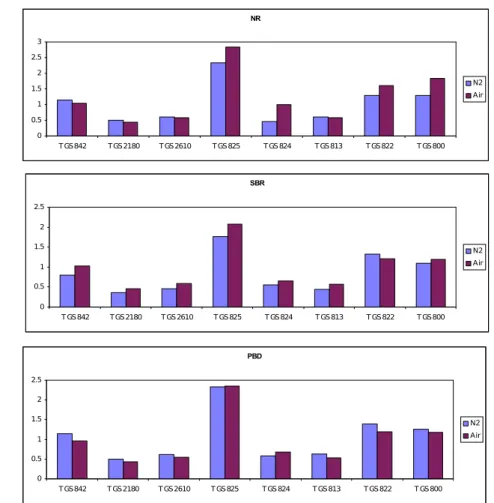
Secondly, the metallic oxide sensors need the presence of oxygen in order to reach an initial equilibrium state. When nitrogen is used as carrier gas, that equilibrium state is reached by a static contact of sensors with ambient air, prior to the pyrolysis itself. When air is used, the initial state results on a dynamic flow on the sensors of the oxygen present in the air, resulting probably in a different response kinetic during the next measurement. Figure 8 shows the responses of the 8 TGS sensors (raw signal, without reference to base line), respectively for NR, SBR and PBD, each time with nitrogen and with air as carrier gas.
The figure shows some differences in the relative behavior of signals when the carrier gas changes. For some sensors, the signal (proportional to the odor intensity) is higher for the air, and for some others, the signal is higher for nitrogen, with variations with respect to the compound (NR, SBR or PBD). This latter remark is interesting in the frame of a possible compound classification. Both carrier gases are user in further tests.
NR 0 0.5 1 1.5 2 2.5 3 T GS 842 TGS 2180 T GS 2610 T GS 825 T GS 824 T GS 813 T GS 822 T GS 800 N2 Air SBR 0 0.5 1 1.5 2 2.5 T GS 842 TGS 2180 T GS 2610 T GS 825 T GS 824 T GS 813 T GS 822 T GS 800 N2 Air PBD 0 0.5 1 1.5 2 2.5 T GS 842 T GS 2180 T GS 2610 T GS 825 T GS 824 T GS 813 T GS 822 T GS 800 N2 Air
Figure 8 : Comparison of signals generated with three samples (resp. NR, SBR and PBD) on the 8 TGS sensors when the carrier gas is either nitrogen or air.
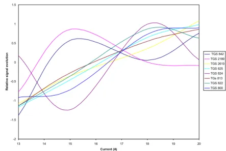
Influence of the laser power on the metallic oxide sensor response
As seen in figure 2, the laser optical power increases about linearly between 0 and 18 W when the current in the laser diode increases from about 7.8 to about 33 A. Of course, the choice of the optimal power for the laser depends on the assembly chosen for the experiments : the beam intensity at the sample level is influenced by the distance from the laser to the sample and by the type of slot and/or frame made in the test box.The only aim of the present test is the optimization of the laser power for efficient gas detection in the limits of the feasibility study.
Figure 9 shows the relative behavior of the signal evolution with the laser current (average for the 3 main compound compositions and for 5 minutes of pyrolysis under nitrogen flow).
-2 -1.5 -1 -0.5 0 0.5 1 1.5 13 14 15 16 17 18 19 20 Current (A) R e la ti v e s ig n a l e v o lu ti o n TGS 842 TGS 2180 TGS 2610 TGS 825 TGS 824 TGs 813 TGS 822 TGS 800
Figure 9 : Relative evolution of the sensor signals versus laser beam current, averaged for the three main compound compositions (vertical axis units are unimportant).
As shown in this figure, some sensor signals (TGS842 and TGS2180) exhibit a maximum for 15 A, some others (TGS824, TGS800, TGS822) saturate or decrease for current exceeding 18 A and the others are strictly growing with the laser beam current. The difference of the signal evolution for the various sensors shows that different components are probably released in the samples when the laser beam power increases. However, the effect of the compound composition on that evolution isn't really significant. When the heat treatment is made with air flow, the signals are generally continuously rising, but with a saturation around 18 A. In consequence, a 18 A laser beam current is chosen for further experiments with the test assembly.
Classification with the NST e-nose
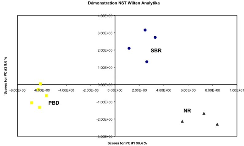
The first classification results concern the tests with an "ideal" instrument, considered as a reference for future development : the Swedish "Emission Analyzer", from NST, distributed in Belgium by Wilten Analytika (Mr Hanse).
The gas produced by the heat treatment on the compound is sampled in Tedlar bags and presented to the NST electronic nose. The heat treatment and the sampling are performed under nitrogen flow, but the operation in the NST detector consists in the measurement of the difference between the "base line", resulting from dry air flow on the sensors, and the signal corresponding to the flow of the gas sample on the sensor array, after 1 minute. A total of twelve runs are performed : 3 with NR, 5 with PBD and 4 with SBR. Figure 10 shows the results of a Principal Component Analysis on the signals coming only from 2 sensors (a MOSFET and a MOS) : the groups are perfectly classified.
It should be mentioned however that those results are obtained after some first unreliable tests carried out with bad operational conditions (position of tubes, valve and extraction needle operation, …), showing that, even with that "ideal" instrument, one should care about the experimental conditions.
Neural Networks give the same kind of results. However, we must insist on the fact that figure 10 refers to PCA analysis, which is an unsupervised procedure : that means that the groups are formed independently of a learning phase. That shows the very good quality of that classification result. At this stage, we may already conclude that a compound composition detector is feasible with this kind of method. Further tests will chiefly be aimed at the simplification of the measurement technique with respect to a commercial instrument.
Démonstration NST Wilten Analytika -3.00E+00 -2.00E+00 -1.00E+00 0.00E+00 1.00E+00 2.00E+00 3.00E+00 4.00E+00
-8.00E+00 -6.00E+00 -4.00E+00 -2.00E+00 0.00E+00 2.00E+00 4.00E+00 6.00E+00 8.00E+00 1.00E+01
Scores for PC #1 90.4 % S c o re s fo r P C # 2 9. 6 % NR PBD SBR
Figure 10 : Principal Component Analysis with 12 compounds samples tested with the NST electronic nose.
Classification with FUL detection system : nitrogen flow, no heat treatment
With the laboratory assembly shown in figure 6, we have first tested as operational variable for the classification mathematical methods the signal supplied by the sensors before the pyrolysis, i.e. when nitrogen just flows over the compound samples, without any smoke generated by the laser beam.The results of the discriminant analysis are shown in figure 11. Obviously, the diagram exhibits a very good discrimination. Thus, the odor simply generated naturally by the compound samples is sufficient to discriminate the composition. Nevertheless, such good classification results obtained only with the surface odor wouldn't probably occur with samples cutted out real used tires.
-8 -6 -4 -2 0 2 4 6 8 -8 -6 -4 -2 0 2 4 6 8 ROOT1 NR SBR PBD Discriminant analysis : learning with 23 samples without
pyrolysis
Figure 11 : Results of discrimant analysis on the natural odor generated by 23 compound samples (without pyrolysis)
Classification with FUL detection system : nitrogen flow, heat treatment
The next classification test uses as operational variables the sensors responses during the heat treatment and under nitrogen flow (later on referred as "pyrolysis"). The laser beam current is 18 A and the carrier gas flow rate is 300 ml/min.The operation consists in waiting an equilibrium state under nitrogen flow (later on referred as "base line"), switching the laser on during 2 minutes , and then continuing to record the signals during the recovery phase, still under nitrogen flow.
The following sets of variables are tested :
S1 : the raw signals after 1 min of pyrolysis
S2 : the raw signals after 2 min of pyrolysis
S3 : the raw signals 1 min after the pyrolysis (3th min of recording)
S5 : the raw signals 3 min after the pyrolysis (5th min of recording)
S7 : the raw signals 5 min after the pyrolysis (7th min of recording)
D1 = S1 – base line
D2 = S2 – base line
D3 = S3 – base line
D5 = S5 – base line
D7 = S7 – base lineThe best discrimination results are obtained with S2 and S3, eventually normalized with respect of the 8 sensors.
Figure 12 shows the representation in the plane of the two discrimination functions of the 31 measurement points related to the 3 main compounds, NR, PBD and SBR, for the variable S2.
-4 -3 -2 -1 0 1 2 3 -6 -5 -4 -3 -2 -1 0 1 2 3 4 5 Root1 Ro ot 2 NR SBR PBD
Figure 12 : Results of the model calibration by discriminant analysis, with 31 compound samples (NR, SBR or PBD) and pyrolysis operation.
As seen in that figure, the classification model is rather well calibrated, although some measurements are misclassified. A total of 87 % of the samples are well classified. In the 13 remaining percent, one "NR" is put in the "SBR" group, two "PBD" are put in the "SBR" group and one "SBR" is put in the "NR" group.
Now, if we try to classify the compound mixtures (NR+PBD, SBR+PBD, NR+SBR and SBR+PBD/C) using the model calibrated as above with only the three main compound compositions, the NR+SBR mixture is always classified in the "NR" group, the NR+PBD mixture is sometimes classified in the "NR" group and sometimes in the "PBD" group, the PBD+SBR mixture is classified either in the "NR" group, or in the "PBD" group, and the SBR+PBD/C is always classified in the "NR" group. The latter result confirms the observation of the laser beam impact on the SBR+PBD/C mixture (see above, the point "Visual distinction").
Finally, the whole set of compound samples, including the mixtures, can be used in the learning phase.
Figure 13 represents the model calibrated with the discriminant analysis for 64 measurements carried out on the 3 main compound compositions as well as on the 4 possible mixtures (still for the "raw" signal, after 2 minutes of pyrolysis). NR PBD SBR NRSBR NRPBD SBRPBD SBRPBDC Root 1 vs. Root 2 Root 1 R o o t 2 -5 -4 -3 -2 -1 0 1 2 3 4 5 6 -8 -6 -4 -2 0 2 4 6
Figure 13 : Results of the model calibration by discriminant analysis, with 64 compound samples (NR, SBR, PBD, NR+PBD, NR+SBR, SBR+PBD or SBR+PBD/C) and pyrolysis operation.
The model leads to a rather good classification, remembering that the above figure shows only the projection on the plane of the first two discrimination functions on a total of 6 functions (and thus hiding a part of the information). But a total of 84.4 % of the samples are well classified. In the 15.6 remaining percent one "NR" is in the "SBR" group, three "PBD" are in the "SBR" group, one "SBR" is in the "NR" group, one "NR+SBR" is in the "SBR+PBD" group, one "NR+PBD" is in the "PBD" group and two "SBR+PBD" are in the "NR+PBD" group.
The discriminant analysis applied on the sensors signals during pyrolysis leads thus to satisfactory results, but not sufficiently reliable to be used for a precise recognition in the field. Moreover, it is awkward to explain the relative location of the groups formed by the discriminant analysis and their relation with the sensor role. In other words, the "signature" of each compound composition, i.e. the pattern formed by the 8 sensors for a given composition, is not typical and constant for all the measurements on the same sample type. The only explanation which could be attempted from the analysis illustrated by figure 12 is that the TGS825 sensor (typical of H2S)
seems reacting more for "NR" compounds and TGS822 sensor (typical of solvents) seems favorable to "PBD" with respect to "SBR". For the analysis including the mixtures (figure 13), the explanation of the sensors role is less obvious.
We may conclude from the test during the pyrolysis operation that a classification should be possible, but it wouldn't be 100 % reliable.
Classification with FUL detection system : air flow, heat treatment
For the next classification test, the heat treatment is carried out under air flow (later on referred as "combustion"). Still, the laser beam current is 18 A and the carrier gas flow rate is 300 ml/min.For the discriminant analysis, the best classification is obtained with S3, i.e. 1 minute after the end of combustion
in the test chamber. That could be explained by the fact that, at that time, the reaction gas reaches the sensor board in a well mixed state.
Figure 14 shows the representation of the 22 measurement points in the plane of the two discrimination functions.
Now, the classification is perfect : 100 % of the samples are well classified and the groups are better separated than in figure 12.
Again, the signal of TGS825 sensor (more sensible to H2S) characterizes the left side of the figure (i.e. "NR"),
together with TGS822 (solvents) and TGS800 (air contaminants), while TGS2180 (water vapor) characterizes more the right side ("artificial compounds"). The vertical separation "PBD"/"SBR" is less easy to explain : TGS825 (H2S) seems more favorable to PBD (the upper part of the figure), while TGS813 (combustible gases)
seems favorable to SBR (lower part).
-6 -5 -4 -3 -2 -1 0 1 2 3 4 -15 -10 -5 0 5 10 Root1 Ro ot 2 NR SBR PBD
Figure 14 : Results of the model calibration by discriminant analysis, with 22 compound samples (NR, SBR or PBD) and combustion operation.
On the basis of the same set of variables, we may also try to classify the compounds using a neural network procedure. Figure 15 shows the network architecture tested. All the neurons are "logsigmoid" ones and the backpropagation algorithm is used.
Figure 15 : Architecture of the neural network tested with the backpropagation algorithm for the classification of compound composition neurone 8 neurone 7 neurone 6 neurone 5 neurone 4 neurone 3 neurone 2 neurone 1 TGS842 signal TGS2180 signal TGS2610 signal TGS825 signal TGS824 signal TGS813 signal TGS822 signal TGS800 signal neurone 9 neurone 10 neurone 11 output = 1 if "NR", 0 otherwise output = 1 if "SBR", 0 otherwise output = 1 if "PBD", 0 otherwise
With that method, if we impose 1-0-0, 0-1-0 or 0-0-1 at the outputs of the three neurons of the output layer, for input signals generated repectively by NR, SBR or PBD, the model calibrated on the basis of the 22 samples recognizes at 100 % the three compound compositions.
Despite of that latter very good result, we shall not use neural network in the future, because it doesn't allow a clear understanding of the physical behavior of the combustion and of the sensors reaction.
At last, in order to appreciate the ability of the sensor array to classify the compounds by itself, a principal component analysis is applied on the data. Figure 16 shows the representation of the measured points in the plane of the two first principal components (90 % of the variability).
-2.5 -2 -1.5 -1 -0.5 0 0.5 1 1.5 2 2.5 -1.5 -1 -0.5 0 0.5 1 1.5 2 Factor 1 Fa ct or 2 NR PBD SBR
Figure 16 : Representation of the 22 measured points in the plane of the two first principal components (90 % of the variability)
The separation is good, despite of some confusion between PBD and SBR. In the case of pyrolysis (nitrogen flow), no separation was visible in the PCA plane. That is an encouraging result which shows the efficiency of the detection principle with those eight sensors, and with air as carrier gas.
Concerning precisely the sensors, a more accurate analysis of the PCA results shows that the right part of figure 16, i.e. the "NR" compound is less under the influence of TGS2180 (water vapor) and TGS842 (methane) than the left part. Nevertheless, it is not possible to identify a subset of the 8 sensors which shouldn't be relevant for the classification purpose : every sensors seems participating to the discrimination.
Before concluding that the method is successful, we have still to validate the calibrated model. Actually, figure 14 shows only the results of the learning (or calibration) phase. The further running phase would consist in using the calibrated model to affect unknown samples to a group.
So, 3 measurements are extracted from the previous data set to be used as validation results : we choose at random one "NR", one "SBR" and one "PBD". Then, we calibrate the model with the discriminant analysis applied on the remaining data set. Moreover, we measure mixtures "NR+SBR", "SBR+PBD", "NR+PBD", "SBR+PBD" and "SBR+PBD/C" and we look at they localization in the root1/root2 diagram.
Figure 17 shows that diagram, calibrated with the 19 remaining samples, with 8 additional points corresponding to validation data (large black circles). To find the position of those points, we used the model previously calibrated, but without telling it the origin of the new samples. As observed, the three pure compound composition samples are well classified, and the compound mixtures are rather logically placed : NR+SBR in the "NR" group, NR+PBD between "NR" and "PBD" (but affected to "NR" group), SBR+PBD in the "PBD" group and SBR+PBD/C in the "NR" group (still confirming the previous results about that compound composition).
That mixtures classification shows that the presence of SBR in a binary compound mixture is generally masked by the effect of the second component.
-4 -3 -2 -1 0 1 2 3 4 5 -20 -15 -10 -5 0 5 10 15 Root1 Ro ot 2 NR PBD SBR NR+SBR NR SBR+PBD/C NR+PBD SBR+PBD PBD SBR
?
?
?
SBR PBD NRFigure 17 : Validation of some cases in the plane of the two discriminant functions.
On sight of figure 17, we may thus conclude that the designed system is able to recognize rather well the compound composition.
Nevertheless, in order to be aware of limitations and of possible improvements concerning the used method, some remarks should be made :
We didn't use the mixtures for the learning phase, that means that we calibrated the model only for three pure compositions. The main reason is the lack of time to carry out all the measurements. But, anyway, the more numerous are the groups, the more difficult the recognition will be, including for the pure composition compounds. For future phases of the study, rather than trying absolutely to classify all the possible mixtures, it should probably be preferable to calibrate the model for pure composition only, and so, at least insuring a good classification for those cases.
The three points labeled with a question mark in figure 17 (black triangles) correspond to doubtful measurements : the signal was not stabilized before the heat treatment (probably due to the interference with other odors in the lab) : those points are misclassified (excepted SBR). That shows the importance of the operational conditions reproducibility. Moreover, for future portable instrument, it will be very difficult to work with an "open" system, which may react to any ambient odor : the proposition would be to supply a continuous "pure" air flow on the sensor array and to "inject" in that flow the gas mixture generated by the heat treatment on the tire samples.
Concerning the misclassification of the "SBR+PBD/C" sample, and the fact that that sample is always considered as of "NR" type, we got an explanation from Goodyear. It seems that there actually was a labelling mistake : the sample is in reality a mixture NR:PBD 70:30 with different Carbon black level. However, that doesn't completely explain why the sample looks really like natural rubber : other NR:PBD samples actually give different results (for example, for other NR:PBD samples, the laser impact on the rubber is typical of the one observed on synthetic rubber).Anyway, that observation validates the used method : the discriminant analysis on the sensors signals localized that "unknown" sample near the NR:PBD one.
Some further tests were also carried out with "new" samples supplied by Goodyear. Although the compound composition was the same as the one of the first sample set, the ageing was different. The first sample set was tested 6 months after the vulcanization (vulcanization on June 6th, 98, test in December 98), and thesecond one was tested only 2-3 months after the vulcanization (vulcanization on October 29th, 98, test in
December 98 and January 99). The measurement points corresponding to the "new" set fall outside the frame of figure 17. Not only the points lies far from the former ones, but the main directions are not correct. Such observation was already made when we tried to classify environmental odors : if the model calibration is made with particular conditions (e.g. high humidity level), further recognition of the same odorous gas measured in other conditions (e.g. lower humidity level) is impossible. Thus, the learning phase must imperatively concern all the possible variants of a given compound. Actually, the "new samples" do not present the same ageing state as the "old" ones, and that is sufficient to justify a new calibration of the model.
In order to verify the latter, we did the training with both sample sets : "old" and "new" ones. Figure 18 shows the Root1/Root2 diagram obtained with the discriminant analysis. Despite of 3 misclassified cases on a total of 34, the results remain rather good, and the natural and synthetic rubbers are still well separated. Notice that there is only a mixing between PBD and SBR groups and that the misclassified cases comes either from the new sample set or from the old one. Notice also that the calibrated model is different from the one which was
built with only the "old" sample set. It is normal : the calibrated model always depends on the data presented
during the learning phase. Nevertheless, the larger the data set is, with a broad range of very different conditions, the more "definitive" the model will be. From a sufficient quantity of data, the model will converge towards a final form which can recognize a compound in any condition.
Anyway, from the latter results, we may observe that the ageing state appreciably influences the sensors reaction, perhaps more than the chemical composition itself.
NR SBR PBD Root 1 R o o t 2 -3.0 -2.5 -2.0 -1.5 -1.0 -0.5 0.0 0.5 1.0 1.5 2.0 2.5 3.0 3.5 -8 -6 -4 -2 0 2 4 6 8 10
Figure 18 : Results of discriminant analysis on samples coming both from the "old" set and from the "new" one.
The conclusion is that the quality of the classification will improve with the system training and the actual misclassification of some validation cases doesn't seem to be a drawback for future development.
But, identifying the real cause of the classification by the sensor array could be more awkward. Indeed, what the sensors "smell" could be the bulk composition of the compound, as expected, but it could be also the effect of vulcanization, or ageing, or something else.
We attempted to verify the real cause of the sensors reaction by adding to the tested samples some other ones which didn't undergo any treatment, like vulcanization.
Figure 19 shows the results of the model validation : discriminant analysis on vulcanized samples and validation with "pure" samples (pointed by arrows).
NR SBR PBD Root 1 vs. Root 2 Root 1 R o o t 2 -6 -5 -4 -3 -2 -1 0 1 2 3 4 5 6 -10 -5 0 5 10 15 20 25 NR NR NR NR PBD PBD PBD PBD SBR SBR SBR SBR SBR
Figure 19 : Discriminant analysis : model calibration with vulcanized samples, validation with "pure" samples (pointed by arrows)
Nearly all points behave like natural rubber, though "NR" points are still rather well separated from synthetic rubber ones. The model always recognizes well the "pure NR" samples, the "pure SBR" points are located too much towards the "NR" direction, but generally remain near the "SBR" group. The "pure PBD" seems completely misclassified : too much towards "NR" and "SBR", and far from the "PBD" group.
Even when the classification model is calibrated with the pure samples, considered as belonging to the input data set, the results are not as good as expected. All the "NR" samples are well classified, but not the synthetic ones. This latter result probably shows that the vulcanization takes a great part in the recognition process.
At last, we tested some vulcanized samples from "unknown" origin, labeled by Goodyear : 464-11, 464-16, R464-16, N545, A78X and 32RY6089-O.
After testing them in the same conditions as previously, we tried to localize the corresponding points in the Root1/Root2 diagram of figure 18 (resulting from the previous calibration, with vulcanized samples).
Again, those new points fall far outside the frame of the diagram, and their location is rather erratic. The only common feature of all those new points is their localization in the "NR" part of the diagram.
However, considering the actual classification method, based on the training of various samples, that result can't be considered necessarily as a bad result.
Again, those new sample types were not took into consideration by the calibrated model. It should be possible to re-calibrate the model with those new samples, but we didn't know to which class (NR, PBD or SBR) the "pure" samples should be assigned.
Anyway, that disturbing result is important for us and suggests to systematically test, in possible further study, the real cause of the discrimination.
Classification with Microsens multisensors system : air flow, heat treatment
The last test concern the same system as the latter one, but with the Microsens multisensor system in place of the array of TGS sensors.As above mentioned, for this first exploratory test, we chose the simplest available multisensor : the 14A08 (see table 3). It is a 4-component multisensor, with sensors 1 and 3 undoped and sensors 2 and 4 Pd-doped. In order to reach a relative selectivity, we chose to operate with different temperature levels for similar sensors. Thus sensors 1 and 2 operate at 500°C (heating voltage : 2.548 V), and sensors 3 and 4 operate at 400 °C (heating voltage : 2.17 V).
As the box containing the multisensor is much smaller than the TGS array one (see photo 3), the time response of the system is also much shorter. Consequently, the operation is somewhat different than previous one. Firstly, the 1-liter heat treatment chamber is filled with the combustion gas (laser diode "on" for 15 seconds). Then, the gas is allowed to flow for 10 seconds on the multisensor in the box.
After that, the multisensor is "cleaned" with pure air for about 2 minutes.
A second puff of combustion gas is injected in the box for a second measurement and so forth. Generally, 4 measurements are so carried out with the same combustion gas.
Figure 20 shows the representation, in the plane of the two discriminant functions, of the 33 measurement points. In spite of poor system optimization (we chose a simple multisensor and, randomly, two temperature levels), the classification is rather good. The figure still exhibits a good separation left/right between natural rubber and artificial one. The separation PBD versus SBR is less obvious : a "SBR" is misclassified in the "PBD" group and a "PBD" is misclassified in the "SBR" group.
NR SBR PBD Root 1 vs. Root 2 Root 1 R o o t 2 -3 -2 -1 0 1 2 3 4 5 -6 -4 -2 0 2 4 6 8
Figure 20 : Discriminant analysis diagram for 33 measurement points with the Microsens multisensor.
Unlike the case of TGS sensors array, it is here difficult to extract the role of each sensor from the results of this discriminant analysis. At first sight, sensors 3 and 4 seems giving redundant information (correlation coefficient close to 1), while the sensor 1 response differs clearly from a compound to another. However, relating that sensor signal to a given chemical family is not straightforward.
Further studies should focus on the optimal choice of multisensor type and operational conditions.
General conclusion and trends
The first and more important concluding remark is that the used principle proves to be efficient for tire compound recognition.
The feasibility study is very promising for further development of a mobile prototype : both the laser heat treatment and the recognition with a gas sensor array are adapted to the set target.
Nevertheless, we must be aware of operational conditions and of some details of the future design :
the heat treatment chamber, where laser beam locally heats the compound, must be sized for a given laser diode and a given laser current;
working with air instead of nitrogen is recommended;
cleaning the sensors with a pure air flow before each measurement is essential;
the sensor array must be optimized for the application (choice of sensor type and of heating voltage and operation);
the reproducibility of operational conditions is of paramount importance : same reference air, same flow rate, same sensor heating voltage, same laser current, same heat treatment duration for every measurement;
the model calibration with discriminant analysis (learning phase) must be carried out with a large number of samples of each type, in all possible conditions;
a miniaturized sensor array, like Microsens multisensors, can be used, but the choice of the right sensible layer and of the right heating voltage must be optimized. That requires accurate and systematic tests of all possible combinations;
the instrument should be periodically updated to take into account new compound compsitions;
a periodical calibration is recommended to minimize the effect of sensor drift;
…The conclusion is thus that such instrument is feasible, but now the real research phase will begin : the test bench used in the frame of this feasibility study is far from being a portable instrument and the lab conditions are far from the workshop one.
The main lesson learnt from the first feasibility phase is the general trend for a future mobile instrument.
Some different solutions could be considered, but the gas sensor array being in the "pyrolysis" chamber in static contact with the generated gas should probably be discarded. Rather, the trend is to work with sensors in a closed box and with dynamic flow. Though the true mobile compact instrument is possible, we should also consider solutions where the generated gas is sampled with some simple device (rubber syringe, …) at the "pyrolysis" level and later on injected in a stand alone detector. Such solution would guarantee more reproducible operational conditions. It would also facilitate the operation with gas sensors which must be continuously heated. In summary, if some rules are respected, notably to reduce interference effects, the design of a compound composition tester using the above described method is workable.
Acknowledgement
The department "Environmental Monitoring" of F.U.L. would like to thank GOODYEAR s.a. for their financial contribution to that research, WILTEN Analytika for placing the NST electronic nose to our disposal and Microsens s.a. in Switzerland for their scientific cooperation when using their sensors.