arXiv:1412.7761v3 [astro-ph.EP] 7 Jan 2015
DISCOVERY OF WASP-85 A b: A HOT JUPITER IN A VISUAL BINARY SYSTEM†
D. J. A. Brown1, 2, D. R. Anderson3, D. J. Armstrong1, F. Bouchy4, 5, A. Collier Cameron6, L. Delrez7, A. P.
Doyle1, M. Gillon7, Y. Gomez Maqueo Chew1, 8, L. Hebb9, G. H´ebrard4, 5, C. Hellier3, E. Jehin7, M. Lendl7, 10,
P. F. L. Maxted3, J. McCormac1, M. Neveu-VanMalle10, 11, D. Pollacco1, D. Queloz11, 10, D. Segransan10, B.
Smalley3, O. D. Turner3, A. H. M. J. Triaud12, 10, and S. Udry10
Draft version January 8, 2015 ABSTRACT
We report the discovery of the transiting hot Jupiter exoplanet WASP-85 A b. Using a combined analysis of spectroscopic and photometric data, we determine that the planet orbits its host star every 2.66 days, and has a mass of 1.09 ± 0.03 MJup and a radius of 1.44 ± 0.02 RJup. The host star is of G5 spectral type, with magnitude V = 11.2, and lies 125 ± 80 pc distant. We find stellar parameters of Teff= 5685 ± 65 K, super-solar metallicity ([Fe/H] = 0.08 ± 0.10), M⋆= 1.04 ± 0.07 M⊙ and R⋆= 0.96±0.13 R⊙. The system has a K-dwarf binary companion, WASP-85 B, at a separation of ≈ 1.5′′. The close proximity of this companion leads to contamination of our photometry, decreasing the apparent transit depth that we account for during our analysis. Without this correction, we find the depth to be 50 percent smaller, the stellar density to be 32 percent smaller, and the planet radius to be 18 percent smaller than the true value. Many of our radial velocity observations are also contaminated; these are disregarded when analysing the system in favour of the uncontaminated HARPS observations, as they have reduced semi-amplitudes that lead to underestimated planetary masses. We find a long-term trend in the binary position angle, indicating a misalignment between the binary and orbital planes. WASP observations of the system show variability with a period of 14.64 days, indicative of rotational modulation caused by stellar activity. Analysis of the Ca ii H+K lines shows strong emission that implies that both binary components are strongly active. We find that the system is likely to be less than a few Gyr old. WASP-85 lies in the field of view of K2 Campaign 1. Long cadence observations of the planet clearly show the planetary transits, along with the signature of stellar variability. Analysis of the K2 data, both long and short cadence, is ongoing. Keywords:planets and satellites: detection – planets and satellites: individual: WASP-85 – techniques:
photometric – techniques: radial velocities
†based on observations (under proposal 089.C-0151(A)) made
using the HARPS high resolution ´echelle spectrograph mounted on the ESO 3.6-m at the ESO La Silla observatory, and the IO:O camera on the 2.0-m Liverpool Telescope under program PL12B13.
1Department of Physics, University of Warwick, Coventry
CV4 7AL
2Astrophysics Research Centre, School of Mathematics &
Physics, Queen’s University, University Road, Belfast, BT7 1NN, UK.
3Astrophysics Group, School of Physical & Geographical
Sci-ences, Lennard-Jones Building, Keele University, Staffordshire, ST5 5BG, UK.
4Institut d’Astrophysique de Paris, UMR7095 CNRS,
Univer-sit´e Pierre & Marie Curie, 98bis boulevard Arago, 75014 Paris, France
5Observatoire de Haute Provence, CNRS/OAMP, 04870 St
Michel l’Observatoire, France.
6SUPA, School of Physics and Astronomy, University of St
Andrews, North Haugh, St Andrews, Fife KY16 9SS, UK.
7Institut d’Astrophysique et de G´eophysique, Universit´e de
Li`ege, All´ee du 6 Aoˆut, 17 (Bˆat. B5C) Sart Tilman, 4000 Li´ege, Belgium
8Instituto de Astronomia, Universidad Nacional Aut´onoma
de M´exico, Circuito Exterior s/n, Ciudad Universitaria, M´exico, D.F., C.P. 04510
9Department of Physics and Astronomy, Vanderbilt
Univer-sity, Nashville, TN 37235, USA
10Observatoire Astronomique de l’Universit´e de Gen`eve,
Chemin des Maillettes 51, 1290 Sauverny, Switzerland
11Cavendish Laboratory, J J Thomson Avenue, Cambridge,
CB3 0HE, UK
12Kavli Institute for Astrophysics & Space Research,
1. INTRODUCTION
The study of extra-solar planets has been driven for-ward by the discovery and detailed analysis of those plan-ets that transit the disc of their host star. These tran-siting systems provide information on the planet’s radius (e.g. Charbonneau et al. 2000) and absolute mass, infor-mation that is vital for the accurate characterisation of both the planet and star. Planets transiting bright stars (8.5 < V < 12.5) are particularly prized; they enable detailed follow-up studies that can provide confirmation of the planets’ existence, as well as allowing the explo-ration of the planets’ characteristics, such as spin-orbit alignment and atmospheric composition.
The space-based Kepler (Borucki et al. 2010) transit survey mission has vastly expanded the size of the ex-oplanet population, and has discovered small, Earth-like planets, circumbinary planets, and multi-planet sys-tems that are inaccessible to instruments on the ground. It is the ground-based surveys though, such as the Wide Angle Search for Planets (WASP; Pollacco et al. 2006), HATnet (Bakos et al. 2002), TrES (Alonso et al. 2004), XO Project (McCullough et al. 2005) , and KELT (Pepper et al. 2007), that are leading the way in the dis-covery of planets orbiting bright stars. WASP is by far the most successful of these surveys, with more than 100 published planet discoveries to date.
A recent study of F, G, and K stars in the Sloan Digital Sky Survey (SDSS) showed that approx-imately 43 ± 2 percent of solar-type stars have binary companions with periods of < 1000 days (Gao et al. 2014). This supports earlier results by Raghavan et al. (2010) (46 ± 2 percent solar type stars in binaries), Duquennoy & Mayor (1991), and Abt & Levy (1976), among others. However, the binary fraction seems to be lower for exoplanet systems (Roell et al. 2012) , indicat-ing a suppression of planet formation (Wang et al. 2014). There is a strong selection effect acting against binary systems in planet search programs, that Roell et al. ac-knowledge and Wang et al. correct for. The presence of a companion star to the planet host introduces the prob-lem of light from said star contaminating either the pho-tometric observations (diluting the transit depth), troscopic observations (introducing a second set of spec-tral lines, and thus a second cross-correlation function peak), or both. The level of contamination depends on several factors - the resolution of the instrument, aper-ture size, fibre diameter, seeing, the separation of the stars, and the magnitude difference between the stellar components. These factors vary considerably from sys-tem to syssys-tem, and the presence of a binary companion to an exoplanet candidate star tends to reduce the likeli-hood of that candidate becoming the target of follow-up observations.
Nevertheless, there are several examples of hot Jupiter exoplanets in S-type orbits around binary stars, in-cluding 70 A b (Anderson et al. 2014); WASP-77 A b (Maxted et al. 2013); WASP-94 A b and B b (Neveu-VanMalle et al. 2014); Kelt-2 A b (Beatty et al. 2012), and Kepler-14 A b (Buchhave et al. 2011). Anal-ysis of the known planets in binary systems deal with the contamination in different ways. For their anal-ysis of WASP-70 A b, Anderson et al. (2014) corrected the photometric data using flux ratios derived from
their observations. A similar approach was taken by Neveu-VanMalle et al. (2014) for WASP-94 A b, and by Maxted et al. (2013) for WASP-77 A. Kepler-14 A b is possibly the most similar system to that we consider here, and Buchhave et al. (2011) account for the dilu-tion by placing a prior on the flux ratio of the binary components. The most complex approach is that of Beatty et al. (2012) for Kelt-2 A b, who carry out an iter-ative combination of Markov Chain Monte Carlo analysis and SED fitting to constrain the transit depth.
In this paper we present the discovery of WASP-85 A b, a transiting hot Jupiter exoplanet with mass Mp= 1.09 ±0.03MJupand radius Rp= 1.44 ±0.02RJup. The solar-type host star, WASP-85 A is the brighter com-ponent of a close visual binary, BD+07◦2474, while the companion star, WASP-85 B, is cooler than the host star, but of similar magnitude. The presence of the com-panion star complicates the standard analysis procedure used for WASP planets; we account for the 3rd light con-tamination by adding an additional term to our stellar model, derived from our photometric data and controlled by a Markov Chain Monte Carlo jump parameter and prior.There is a clear, long-term trend in the position angle between the binary components, which indicate an orbit of ≈ 3000 years for the binary. The system lies in the field of view of K2 Campaign 1, and was observed in both long and short cadence modes. The K2 light curve clearly shows the planetary transits, along with the sig-nature of stellar variability. Analysis of the K2 data from both observing modes is ongoing, and will be presented in a follow-up paper.
In Section 2 we detail the photometric and spectro-scopic observations of the WASP-85 system, while in Section 3 we discuss the methods by which we derive the system parameters. We discuss the characteristics of the star and planet in Section 4, and conclude by summaris-ing our results in Section 5. Throughout the manuscript we use the TDB time standard and Barycentric Julian Dates in our analysis, following the advice set out in Eastman, Siverd, & Gaudi (2010). Our results are based on the equatorial solar and jovian radii, and masses taken from Allen’s Astrophysical Quantities.
2. OBSERVATIONS 2.1. WASP photometry
For a detailed account of the WASP telescopes, observ-ing strategy, data reduction, and candidate identification and selection procedures, see Pollacco et al. (2006, 2008) and Collier Cameron et al. (2007).
BD+07◦2474 lies near the celestial equator, and was thus observed by both SuperWASP-North (located at the Observatorio del Roque de los Muchachos on La Palma, Spain) and WASP-South (located at the South African Astronomical Observatory near Suther-land, South Africa). These observations resulted in 20936 data, spanning the period 2008-02-05 to 2011-03-29.
The system was first identified as a planet candidate from SuperWASP-North data in 2008. Initial analysis revealed transit like features with an apparent period of ≈ 1.59 days. This signal was subsequently identified in both the SuperWASP-North and WASP-South photom-etry independently, and the star was selected for
photo-metric and spectroscopic follow-up observations. Subse-quent to these observations, the secondary peak in the periodogram, at ≈ 2.66 days, was found to be the correct period.
The radius of the synthetic aperture (48′′) used to extract the flux of BD+07◦2474 is much greater than the maximum binary separation (1.8′′; see Section 4.2), such that the WASP lightcurve includes flux contribu-tions from both components of the binary.
2.2. Spectroscopic follow-up
Initial spectroscopic reconnaissance was carried out be-tween 2008 and 2010 using the SOPHIE spectrograph (Perruchot et al. 2008; Bouchy et al. 2009) mounted on the 1.93-m telescope of the Observatoire de Haute-Provence (OHP), resulting in the acquisition of 11 spec-tra. RVs were derived through cross-correlation with a spectral mask suitable for a star of G2 spectral type. The separation of the binary components is smaller than the fibre diameter of SOPHIE (3′′), and thus the radial velocities (RVs) obtained from this instrument are con-taminated by the contribution of the companion. These data show a sinusoidal variation in radial velocity (RV) with a period of ≈ 2.66 days, in disagreement with the period identified in the WASP lightcurves.
Further spectroscopic observations were made using the fibre-fed CORALIE spectrograph at the Euler-Swiss telescope at ESO’s La Silla observatory, and using HARPS at the ESO 3.6 m telescope, also at La Silla. A total of 31 observations were made using CORALIE between 2009 January 03 and 2014 June 24. For de-tails of the instrument and data reduction procedure, see Queloz et al. (2000) and Wilson et al. (2008). RVs were derived using cross-correlation with a spectral mask suit-able for a G2-type star, and confirmed the ≈ 2.66 day period as the correct one. Unfortunately, while the CORALIE guiding camera is able to identify the presence of both stellar components, the aperture of the spectro-graph (2′′) is insufficiently small to access a single stellar component at a time. The CORALIE spectra are there-fore also contaminated by light from the companion star. The level of contamination is seeing dependent owing to the close similarity of the aperture size and binary sepa-ration, rendering a correction to the RVs both uncertain and difficult to make.
Eight observations of the brighter binary compo-nent (hereafter WASP-85 A), and five observations of the fainter companion star (hereafter WASP-85 B) were made using HARPS. The small spectrograph aperture (1′′diameter) and good seeing allowed the components to be observed separately, with little contamination from the other star. RVs were extracted in the same manner as for the CORALIE observations.
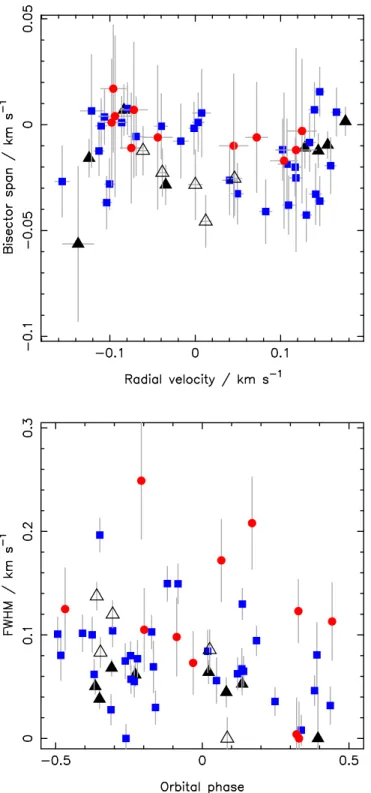
We check for false positives induced by background eclipsing binaries or stellar activity by examining the bisector span measurements for our data. We find no significant correlation with the radial velocities or the radial velocity residuals, although the observations for WASP-85 B do seem to show a negative correlation be-tween the parameters. This is indicative of stellar activ-ity (Queloz et al. 2001). We also plot the full widths at half maximum (FWHM) of our radial velocity ob-servations as a function of orbital phase, checking for variations in phase (Santerne, Moutou, & Bouchy 2011).
None are seen (see Figure 1). We confirm which binary component is the planet host by checking for phasing of the HARPS radial velocity observations. The observa-tions of WASP-85 A show variaobserva-tions in phase with both the photometry, and with the CORALIE and SOPHIE observations, while the observations of WASP-85 B show variations that are not correlated with the phase deter-mined from the lightcurve.
We list our RV data in Table 1, along with the bisec-tor spans, which measure the asymmetry of the cross-correlation functions (CCFs), and the FWHMs of the CCFs. Uncertainties on the bisectors were taken to be twice the uncertainty on the RV, while those on the FWHMs were taken to be 2.35 times the RV uncertainty.
2.3. Photometric follow-up
Follow-up photometric observations to solidify the planet’s ephemeris, and check for transit timing shifts, were carried out using the James Gregory Telescope (JGT) at the University of St Andrews Observatory, the robotic Transiting Planets and Planetesimals Small Telescope (TRAPPIST; Jehin et al. 2011) at La Silla, the Euler-Swiss telescope using EulerCam (Lendl et al. 2012), also at La Silla, and the Liverpool Telescope (LT; Steele et al. 2004) on La Palma using the IO:O instru-ment. These observations are summarised in Table 2.
The resolutions and pixel scales of the telescopes and instruments used for photometric follow-up were insuffi-cient to distinguish the companion star. All lightcurves are therefore of the blended combination of light from the two stellar components.
3. ANALYSIS 3.1. Stellar parameters
We co-added all of the individual HARPS spectra of WASP-85 A and WASP-85 B to produce a single spec-trum with a typical S/N of around 60:1 and 30:1, re-spectively. The standard pipeline reduction products were used in the analysis, which was performed using the methods given in Doyle et al. (2013). The effective temperature (Teff) was determined from the excitation balance of the Fe i lines. The Na i D lines, the Ca i line at 6439 ˚A, and the ionisation balance of Fe i and Fe ii were used as surface gravity (log g⋆) diagnostics. The metallicity was determined from equivalent width measurements of several unblended lines. A value for microturbulence (ξt) was determined from Fe i using the method of Magain (1984).
The projected stellar rotation velocity (v sin I⋆) was determined by fitting the profiles of several unblended lines. Values for macroturbulence (vmac) of 2.93 ± 0.73 and 2.20 ± 0.73 km s−1 were determined from the cali-bration of Doyle et al. (2014). A best fit value of v sin I⋆ = 3.41 ± 0.89 and 3.32 ± 0.82 km s−1 were obtained for WASP-85 A and WASP-85 B, respectively.
The results are summarised in Table 3; the quoted un-certainties account for the errors in Teff and log g⋆ as well as the additional scatter induced by measurement and atomic data uncertainties. The spectral type was es-timated from Teff using Table B.1 in Gray (2008), while the stellar mass and radius estimates were derived using the Torres et al. (2010) calibration.
Table 1
Radial velocity data of WASP-85 A and WASP-85 B, obtained using HARPS, and of the two components combined, obtained using SOPHIE and CORALIE.
BJDTDB RV σRV Bisector σbis FWHM σFWHM −2450000 (days) (km s−1) (km s−1) (km s−1) (km s−1) (km s−1) (km s−1) SOPHIE 4820.64118 13.579 0.024 −0.012 0.048 10.100 0.056 4821.64438 13.367 0.019 0.004 0.0038 10.059 0.045 4822.60638 13.506 0.017 −0.010 0.034 9.976 0.040 4823.61708 13.565 0.016 −0.017 0.032 9.949 0.038 4824.70288 13.365 0.015 0.017 0.030 9.855 0.035 4824.72498 13.363 0.015 0.001 0.030 9.851 0.035 4834.64438 13.417 0.017 −0.006 0.034 10.023 0.040 4835.64718 13.389 0.016 0.007 0.032 9.964 0.038 4836.60168 13.586 0.017 −0.003 0.034 9.956 0.040 5304.44298 13.533 0.013 −0.006 0.026 9.924 0.031 5305.39608 13.386 0.013 −0.011 0.026 9.974 0.031 CORALIE 4834.834967 13.42322 0.00643 −0.00053 0.01286 8.91982 0.01511 4836.811531 13.58281 0.00719 −0.03262 0.01438 8.93960 0.01690 5675.670857 13.67921 0.00577 0.01552 0.01154 8.87000 0.01356 5676.638783 13.42716 0.00652 0.00368 0.01304 8.85258 0.01532 5677.666565 13.53687 0.00696 0.00109 0.01382 8.89084 0.01636 5679.634306 13.42072 0.00577 −0.01245 0.01154 8.82570 0.01356 5684.661489 13.42964 0.00617 −0.03682 0.01234 8.85497 0.01450 5706.548896 13.45416 0.00613 0.00763 0.01226 8.83622 0.01441 5707.572297 13.67309 0.00644 0.00705 0.01288 8.84507 0.01513 5712.520574 13.53203 0.00614 −0.00174 0.01228 8.85190 0.01443 5715.509353 13.67937 0.00582 −0.03608 0.01164 8.84725 0.01368 6020.746523 13.69205 0.00663 −0.01937 0.01326 8.89409 0.01558 6030.562877 13.41197 0.01331 0.00647 0.02662 8.87074 0.03128 6031.594135 13.65143 0.00757 −0.02514 0.01514 8.86701 0.01779 6031.738294 13.64104 0.01067 −0.01863 0.02134 8.85919 0.02507 6032.538879 13.37756 0.00838 −0.02683 0.01676 8.85724 0.01969 6067.600608 13.44722 0.00618 0.00095 0.01236 8.79800 0.01452 6068.533616 13.66361 0.00625 −0.04270 0.01250 8.81772 0.01469 6069.488518 13.46423 0.00933 −0.00556 0.01866 8.84598 0.02193 6070.519073 13.49368 0.00767 −0.00073 0.01534 8.82180 0.01802 6071.591742 13.65052 0.00686 −0.02006 0.01372 8.81989 0.01612 6116.471681 13.69886 0.00569 0.00593 0.01138 8.79002 0.01337 6339.779756 13.66741 0.00689 −0.00840 0.01378 8.89293 0.01619 6341.810736 13.61604 0.00753 −0.04102 0.01506 8.89167 0.01770 6342.674625 13.57377 0.00815 −0.02626 0.01630 8.93949 0.01915 6362.859062 13.54098 0.01032 0.00550 0.02064 8.87031 0.02425 6365.798530 13.63578 0.00726 −0.01186 0.01452 8.89014 0.01706 6366.844086 13.51656 0.00874 −0.00777 0.01748 8.87421 0.02054 6697.826971 13.64283 0.00695 −0.03800 0.01390 8.98653 0.01633 6741.736317 13.43313 0.00603 −0.02803 0.01206 8.88454 0.01417 6833.496459 13.67453 0.00717 −0.03279 0.01434 8.86483 0.01685 HARPS star A 6020.588912 13.74735 0.00316 −0.00958 0.00632 7.59818 0.00743 6020.736685 13.76810 0.00337 0.00149 0.00674 7.61603 0.00792 6028.594310 13.73631 0.00405 −0.01231 0.00810 7.58601 0.00952 6029.582170 13.55755 0.00467 −0.02840 0.00934 7.61188 0.01097 6029.742186 13.50857 0.00598 0.00692 0.01196 7.59248 0.01405 6030.572124 13.45497 0.01833 −0.05632 0.03666 7.54788 0.04308 6031.573927 13.72069 0.00478 −0.01092 0.00956 7.60938 0.01123 6032.541680 13.46784 0.00449 −0.01581 0.00898 7.60061 0.01055 HARPS star B 6020.602442 13.07700 0.00573 −0.01224 0.01146 7.90081 0.01347 6020.745898 13.09952 0.00558 −0.02263 0.01106 7.88332 0.01311 6028.603233 13.15039 0.00614 −0.04569 0.01228 7.84657 0.01443 6029.591232 13.13818 0.00822 −0.02829 0.01644 7.84906 0.01932 6029.750461 13.18411 0.00863 −0.02544 0.01726 7.76341 0.02028
Figure 1. Upper panel: Radial velocity bisector span plotted as a function of relative radial velocity. The uncertainties in the bisector measurements are taken to be 2.0 × σRV. HARPS data
for WASP-85 A are denoted by solid, black triangles, data for WASP-85 B by open, black triangles. CORALIE data are denoted by solid, blue squares. SOPHIE data are denoted by solid, red circles. Only the WASP-85 B data show a negative correlation between the two parameters. Lower panel: Radial velocity full width at half maximum (FWHM) as a function of orbital phase. The uncertainties in the FWHMs are taken to be 2.35 × σRV. The
FWHM values have been offset from the minimum value for each data set to allow comparison. There is no clear variation with orbital phase.
Table 2
Summary of photometric follow-up observations.
Instrument Date Time of observations Filter Ndata
JGT 2009-03-20 21 : 43 − 01 : 42 Cousins R 237 IO:O 2013-01-12 02 : 39 − 06 : 41 Sloan z′ 146 IO:O 2013-01-28 01 : 18 − 05 : 15 Sloan z′ 146 EulerCAM 2013-03-23 04 : 23 − 07 : 55 RG 186 TRAPPIST 2013-03-31 03 : 39 − 08 : 07 Sloan z′ 569 TRAPPIST 2013-04-16 01 : 56 − 06 : 41 Sloan z′ 615 TRAPPIST 2013-05-09 23 : 52 − 04 : 10 Sloan z′ 503 TRAPPIST 2013-05-25 22 : 47 − 03 : 02 Sloan z′ 626
Note: The RG filter used in EulerCAM is a modified broad Gunn-R filter, with a central wavelength of 660 nm.
A slewing problem affected TRAPPIST during the transit on 2013-03-31, leading to gaps in coverage.
Table 3
Summary of the stellar parameters derived using spectroscopic analysis.
Parameter WASP-85 A WASP-85 B Units
RA 11h43m38.01s J2000 DEC +06◦33′49.4′′ J2000 V 11.2 11.9 Tycho B −V 0.670 ± 0.022 0.828+0.034−0.036 Distance 125 ± 80 pc Spectral type G5 K0 Teff 5685 ± 65 5250 ± 90 K Mass, M⋆ 1.04 ± 0.07 0.88 ± 0.07 M⊙ Radius, R⋆ 0.96 ± 0.13 0.77 ± 0.13 R⊙ log g⋆ 4.48 ± 0.11 4.61 ± 0.14 cgs ξt 0.6 ± 0.1 0.9 ± 0.1 km s−1 vmac 2.93 ± 0.73 2.20 ± 0.73 km s−1 v sin I⋆ 3.41 ± 0.89 3.32 ± 0.82 km s−1 Prot 14.6 ± 1.5 days log A(Li) 2.19 ± 0.06 < 0.70 ± 0.10 [Fe/H] 0.08 ± 0.10 0.00 ± 0.15 log(R′ hk) −4.43 +0.06 −0.02 −4.37 +0.09 −0.04
Note: Masses and radii estimated using the calibration of Torres et al. (2010). Spectral Type estimated from Teff using
Ta-ble B.1 in Gray (2008). Abundances are relative to the solar val-ues obtained by Asplund et al. (2009). The rotation period is the mean of the periods determined from a periodogram analysis of the WASP lightcurve.
3.1.1. Stellar activity
Using the HARPS spectra with S/N > 4 for the core of the Ca ii H+K lines, we calculate the log(R′
hk) activity index using the emission in the cores of the Ca ii H+K lines following Noyes et al. (1984). We find an activ-ity index of log(R′
hk) = −4.43 +0.06
−0.02 for WASP-85 A. For WASP-85 B we find log(R′
hk) = −4.37 +0.09
−0.04using spectra with S/N > 2.
We carried out a search for stellar modulation in the WASP lightcurve using the method described in Section 4 of Maxted et al. (2011). The WASP data were sepa-rated according to the year of observation, as starspot
Table 4
Results from the periodogram analysis of the four seasons of WASP data for the WASP-85 system.
Year Ndata Period Amp FAP
(days) 2008 2559 6.644 0.003 0.0389 2009 6760 15.600 0.003 0.0011 2010 8157 13.130 0.003 0.0000 2011 2442 16.550 0.003 0.0002 Adopted 14.6 ± 1.5
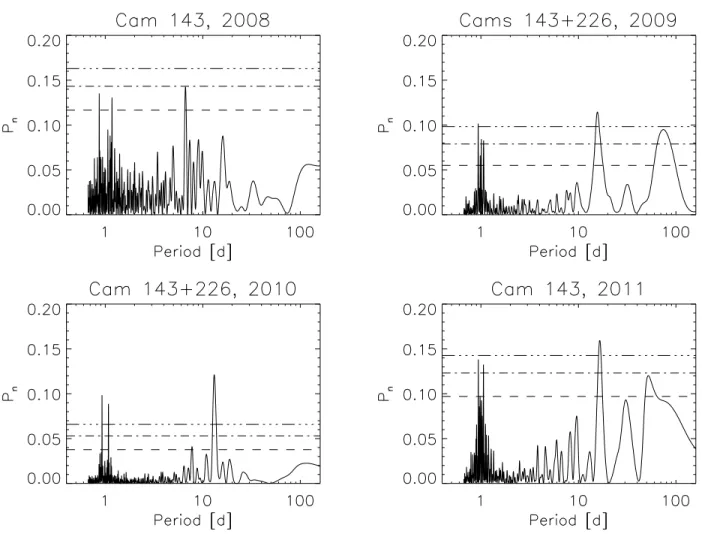
induced variability is not expected to be coherent on long timescales owing to the short lifetime of magnetic fea-tures on the the stellar surface. The transit feafea-tures were subtracted using the best fit model transit model for that year. A modified, generalised Lomb-Scargle periodogram (e.g. Zechmeister & K¨urster 2009), computed using the method of Press & Rybicki (1989) over 4096 uniformly spaced frequencies from 0 to 2.5 cycles/day, was used to search for significant periodicity in the lightcurves. The resulting periodograms are shown in Figure 2, and the results for the most significant peak are given in Table 4. False alarm probabilities (FAP) were calculated using a Monte Carlo bootstrap method (Maxted et al. 2011).
In the 2009, 2010, and 2011 data there are significant peaks at approximately 15 days. We associate this with the stellar rotation of one of the stellar components. The shorter period found in the 2008 data is approximately Prot/2, and easily explained by the presence of two ac-tive regions on opposite sides of the star. This would produce a photometric signature at twice the rotational frequency, and will contribute power in other seasons as well, but less dominantly. Note that there is significant power at periods close to 1 day in all four seasons. This likely arises as a result of the diurnal observing schedule forced upon WASP by its ground-based nature.
We estimate a mean rotation period of 14.6 ± 1.5 days using the results from all four seasons. This value is in good agreement with the rotation period of 14.2 ± 4 d implied by the values of v sin I⋆ and the stellar radius of WASP-85 A. However it is also in agreement with the rotation period of 11.7 ± 4 days implied for WASP-85 B, making it impossible to determine which star the rota-tional modulation originates from using this data alone. We will discuss this result further in Section 4.
We whiten the four sets of data by fitting a harmonic series with P0= Prot/2 as the fundamental period. The number of terms in the series was determined by minimis-ing the Bayesian Information Criterion (Schwarz 1978). The resulting fit was divided-out, and the lightcurves concatenated to produce a whitened WASP lightcurve.
3.1.2. Stellar age
Lithium is detected in WASP-85 A, with an equiva-lent width of 53 m˚A, corresponding to an abundance of log A(Li) = 2.19 ± 0.06. This implies an age of be-tween 0.5 and 2.0 Gyr. There is no significant detection of lithium in WASP-85 B, with an equivalent width
up-Table 5
Age constraints for the two binary components, as determined using a variety of techniques.
Method Ages WASP-85 A WASP-85 B (Gyr) (Gyr) Lithium abundance log A(Li) 0.5 − 2.0 > 0.6 Isochrone placement Padova 0.68+0.88−0.64 > 0.08 YY 1.33 − 2.57 − DSED 2.42+2.27−1.91 − GARSTEC 2.2 ± 1.6 − Gyrochronology Prot 1.53+0.32−0.28 v sin I⋆ < 1.45+1.25−0.58 < 0.81 +0.61 −0.30 Activity Mamajek 0.37+0.09−0.15 0.26 +0.12 −0.16
per limit of 2 m˚A, corresponding to an abundance upper limit of log A(Li) < 0.70 ± 0.10, and implying an age of several Myr (Sestito & Randlich 2005).
Stronger age constraints can be evaluated through a comparison to theoretical stellar models. We use the isochrone placement method of Brown (2014), work-ing in the [ρ−1/3⋆ , Teff] parameter space suggested by Sozzetti et al. (2007). We evaluate the age of each com-ponent using three sets of stellar models: the Padova models of Marigo et al. (2008); Girardi et al. (2010); the Yonsei-Yale (YY) isochrones of Demarque et al. (2004)), and models from the Dartmouth Stellar Evolu-tion Database (DSED; Dotter et al. 2008). We used in-dependent measurements of Teff (derived from the stellar spectra) and ρ⋆ (derived directly from the photometric lightcurves during the transit modelling process, see Sec-tion 3.2) to derive the stellar ages at the central value of [Fe/H] listed in Table 3, and at its 1σ limits. The results are listed in Table 5.
We also carry out a Bayesian isochrone fitting process in [log(L⋆), Teff] parameter space, using the GARSTEC models of Weiss & Schlattl (2008), as computed by Serenelli et al. (2013). This new method is detailed in Maxted, Serenelli & Southworth (2014) . Using this method we find an age of 2.2 ± 1.6 Gyr for WASP-85 A using [Fe/H] = 0.10.
In addition, we estimate the age of the two components using their measured and estimated rotation periods. We use the gyrochronology formulation of Barnes (2010), cal-culating the convective turnover timescale using Table 1 of Barnes & Kim (2010) and setting P0 = 1.1 d. Using the measured rotation period, we derive a gyrochrono-logical age of 1.53+0.32−0.28Gyr. It is also possible to derive gyrochronological ages using the projected rotation ve-locity to derive an upper limit on the rotation period. Ages derived in this manner will also therefore be up-per limits. The rotation rate (Prot= 14.2 ± 4 d) implied
Figure 2. Periodograms for the four seasons of WASP data for the WASP-85 system. The year is given in the title of each panel. The horizontal lines indicate false-alarm probability levels of FAP = 0.1, 0.01, and 0.001. Note the changing scale of the y-axis. In 2009, 2010, and 2011, a significant peak is seen at approximately 15 days. We associate this with the rotation period of one of the stars, though it is impossible to determine which star given the data available. The strongest peak in the 2008 data is at approximately half of this period.
by the measured v sin I⋆ for WASP-85 A gives an age of < 1.45+1.25−0.58Gyr, in good agreement with this. The im-plied rotation rate (Prot = 11.7 ± 4 d) for WASP-85 B gives an age of < 0.81+0.61−0.30Gyr, which would seem to im-ply that the detected rotation period is that of WASP-85 A. However, given the contamination of the WASP photometry we cannot be certain.
Finally, we estimate the age for the two com-ponents using the stellar activity - age relation of Mamajek & Hillenbrand (2008). We find ages of 0.37+0.06−0.14Gyr and 0.24+0.09−0.13Gyr for stellar components A and B, respectively.
The ages for WASP-85 A that we derive using the four different isochrone analyses are consistent, and are also in agreement with the gyrochronology ages that we derive from the detected rotation period, and from v sin I⋆. The age that we determine using the chromospheric activity index is younger than many of the other estimates, but does agree with the Padova isochrone age.
If we assume that the stars are gravitationally bound, as seems likely given the similar radial velocities that we measure for the two stars, and the fact that we see only a single CCF in the CORALIE and SOPHIE spectrum,
then it is encouraging that the results for the two stars agree. We note though that the constraints on WASP-85 B’s age are very loose.
3.2. Planetary and orbital parameters
To determine the planetary and orbital parameters, we carry out a simultaneous analysis of the HARPS RVs for WASP-85 A, and the full suite of photometric observa-tions. This allows us to fully account for inter-parameter correlations, and properly characterise the uncertainties in the system parameters. We elect not to include the RV data obtained using CORALIE and SOPHIE owing to the aforementioned, unknown contamination caused by the presence of the companion star. It is possible to cor-rect the contaminated RVs through careful analysis of the CCFs, given that we have data for the two components separately from HARPS observations. Buchhave et al. (2011) describe another means by which contaminated CCFs can be corrected that applies shifts to the spec-trum and co-adds the results to the observed specspec-trum divided by a constant determined by the flux ratio. Given our access to uncontaminated HARPS data we elect not to perform a correction; we leave this as a problem for a more detailed follow-up analysis of the system in the
Figure 3. Hertzsprung-Russell digram showing the results of a Bayesian analysis of WASP-85 A’s age. The red, solid lines represent isochrones of 0.0, 1.08, and 2.66 Gyr, while the green, dashed lines represent represent evolutionary models of 0.98, 1.02, and 1.06 M⊙, all computed for [F e/H]initial= 0.10. Black dots
mark individual steps in the Markov chain; we display only a random selection of 1000 data to improve clarity.
future.
We carry out our analysis using a modified version of the Markov Chain Monte Carlo (MCMC) code described in Collier Cameron et al. (2007), Pollacco et al. (2008), and Brown et al. (2012). To recap, this models the RVs with a Keplerian orbit, while the transits are fitted using the photometric model of Mandel & Agol (2002). We ac-count for limb-darkening using a non-linear model with four components; we derive wavelength appropriate co-efficients for each photometric dataset by interpolating through the tables of Claret (2000, 2004) at each MCMC step. We also carry out a linear decorrelation in phase at each step to remove systematic trends in the photomet-ric data; owing to the presence of an additional trend in the LT / IO:O lightcurves (probably secondary ex-tinction), we found it necessary to use a quadratic decor relation in phase for the two lightcurves obtained with that instrument. We add an additional stellar “jitter” term of 7.5 m s−1to the formal RV uncertainties in order to obtain a reduced spectroscopic χ2
≈ 1.
The following jump parameters are used as standard: the epoch of mid-transit, T0; the orbital period, P ; the full transit duration, Tdur; the planet:star area ratio, R2
p/R2⋆; the impact parameter for a circular orbit, b; Teff; [Fe/H], and the RV semi-amplitude, K. We apply pri-ors on v sin I⋆ Teff and [Fe/H] using the spectroscopic values listed in Table 3, in all cases assuming a Gaussian distribution. Steps are accepted using the Metropolis-Hastings algorithm, with a scale factor set to ensure an acceptance rate of roughly 25 percent.
For WASP-85, we add a number of additional jump pa-rameters equal to the number of photometric datasets. These are the third light contributions to each transit, L3,i, defined as the flux ratio of the two components FB/FA, and allow us to account for the dilution induced by the presence of the binary companion. We apply a Bayesian prior on each of the L3,i, assuming a Gaussian distribution; for the observations in the Sloan z′band we use the flux ratio of 0.54 ± 0.02 measured in the course
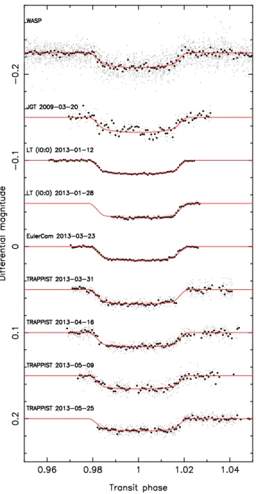
Figure 4. Photometric transit lightcurves of the WASP-85 system. The data have been phase folded using the best fit orbital period and epoch for WASP-85 A b, and binned using a bin width equivalent to 180 s. We plot the original data in grey, and the best fit transit model in red. The lightcurves have been offset for clarity; for the same reason, we omit the error bars. The telescope, instrument, and date of observation are listed alongside each lightcurve. A slewing problem is responsible for the gaps in the lightcurve obtained by TRAPPIST on 2013-03-31.
of the IO:O observations, while for the Cousins R and RG filters we scale this ratio assuming perfect blackbody emission for the two stars. The third light contribution is added to the photometric transit model following the example of Southworth (2010). L3 is strongly correlated with several other parameters, but we are able to model it in this fashion thanks to the measurement from IO:O. We test for the presence of a long-term trend in RV using the additional jump parameter dγ/dt, the rate of
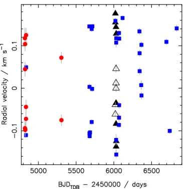
Figure 5. Radial velocity as a function of time. The best fit values of γi have been subtracted from each set of data. Despite
the strong trend identified in our fit, we see no evidence for such trend over the full timespan of our observations. We conclude that the trend in γHARPSarises owing to the very short baseline
of the HARPS observations.
change in systemic velocity with time. We find a sig-nificant improvement in the spectroscopic fit (param-eterised using χ2
reduced) when including such a trend, which we measure at −110 ± 3 m s−1yr−1. However, we are sceptical that such a trend truly exists. The timespan of the HARPS observations is only twelve days, covering just over 4.5 orbits. This is insufficient to truly constrain any trend that might be present in the systemic velocity. Moreover, the CORALIE and SO-PHIE data show no signs of any shift in γ over time. Even with the dilution caused by WASP-85 B, a trend of −110 ± 3 m s−1yr−1 would be easily identifiable in Figure 5, as those data cover nearly 2000 days, over five years, and the postulated trend is on the order of the detected semi-amplitude. We therefore do not fit a trend in our final solution.
To test for an eccentric orbit, we use additional jump parameters of √e cos ω and√e sin ω, where e is the or-bital eccentricity and ω is the argument of periastron. We find eccentricities of between 0.0763 and 0.1774, de-pending on the inclusion or otherwise of a trend, and on whether the Bayesian penalty on stellar radius was applied. All are consistent with zero at < 2σ. We test the significance of these eccentricities using the F-test of Lucy & Sweeney (1971) to compare the fit to that of a circular orbit. We find that the probability of the ec-centricity being detected by chance varies between 0.79 to 0.06, and therefore adopt a circular orbit in line with the advice in Anderson et al. (2012). Once again, the short timespan of the HARPS observations provides in-sufficient constraint even if the eccentricity was found to be significant.
One of the HARPS RV data has an uncertainty three times that of the other measurements, and a bisector span that is twice as large as the next greatest value. We carried out runs omitting this datum to check that it was not biasing our results. We found that removing this point made little difference to the significance of ec-centricity, which we still find to favour a circular orbit but to be more significant in the absence of a long-term trend. Removing the datum led to only a small increase in the value of the fitted trend in γ. We note though that the eccentricity of the orbit tended to increase with the removal of the highly uncertain HARPS measurement. We attribute this to the spacing of the RV data in or-bital phase, which leads to a fit dominated by the three data between phase 0 and phase 0.2.
The system parameters that we adopt are listed in Ta-ble 6, along with the prior values. In Figure 4 we display the phase-folded photometric lightcurves, overlaid with the best fit transit model. Note that the visible transit depth is shallower than the depth listed in Table 6 ow-ing to the effect of the third light contribution. There is a notable difference in scatter between the two LT / IO:O lightcurves. This is likely to be a result of the comparison stars that were available for the data reduc-tion process. For the lightcurve obtained on the night of 2013-01-12 there were two suitable comparison stars, which were fainter than than WASP-85 by factors of 1.8 and 2.25. For the lightcurve obtained on the night of 2013-01-28, only one comparison star was available, and it was four times fainter than our target.
In Figure 6 we plot our RV data, overlaid with the best fit Keplerian orbit model for HARPS only analysis. We show all of our RV data to illustrate the effect of the dilution on the CORALIE and SOPHIE observations. The primary effect is a reduction in the semi-amplitude of the data (see also Table 6), though there is also increased scatter compared to the HARPS observations. We also show the residuals of the data compared to the plotted HARPS model. The sinusoidal structure present in the residuals for the CORALIE and SOPHIE data clearly indicates the reduced semi-amplitude.
This reduced semi-amplitude for the CORALIE and SOPHIE data is expected given the cross-correlation method by which we derive their RV measurements. WASP-85 B is relatively constant in RV, and thus the peak of the CCF will be constant in velocity space. The CCF for WASP-85 A, however, will move in velocity space. The close proximity of the two spares means that these CCFs merge to form a single, asymmetric CCF. The peak velocity will be biased towards the stationary position of WASP-85 B, effectively reducing the shift in velocity induced by the planet, and leading to a smaller semi-amplitude.
4. DISCUSSION 4.1. Diluted observations
We test the effect of the dilution on the parameters that we determine by carrying out several different anal-yses. We start by fitting the photometry and HARPS RVs using the same initial conditions, but without the additional third light term for the photometry. This run finds a transit depth of 0.0132 ± 0.0001, some 50 percent smaller than the depth when accounting for the
contam-Table 6
System parameters for WASP-85 A and WASP-85 A b. We also list the Bayesian priors applied in the course of the MCMC analysis.
Parameter Symbol Value Units
Priors
Projected rotation velocity v sin I⋆ 3.41 ± 0.89 km s−1
Effective temperature Teff 5685 ± 65 K
Metallicity [Fe/H] 0.08 ± 0.10 dex
Flux ratio L3 0.50 ± 0.02 Cousins R filter
Flux ratio L3 0.50 ± 0.02 RG filter
Flux ratio L3 0.54 ± 0.02 Sloan z′ filter
Model parameters
Orbital period P 2.6556734 ± 0.0000008 days
Epoch of mid-transit t0 6311.02659 ± 0.00010 BJDTDB
Transit duration Tdur 0.1118 ± 0.0003 days
Planet:star area ratio R2
p/R2⋆ 0.0265 ± 0.0007
Impact parameter b 0.044+0.037−0.028
RV semi-amplitude KHARPS 172.7 ± 4.8 m s−1
KCORALIE† 132.8 ± 1.7 m s−1
KSOPHIE† 112.5+6.2−6.5 m s−1
Systemic velocity γHARPS 13.5922 ± 0.0032 km s−1
γCORALIE† 13.5335 ± 0.0013 km s−1
γSOPHIE† 13.4610 ± 0.0045 km s−1
Effective temperature Teff 5920+49−58 K
Metallicity [Fe/H] 0.10 ± 0.10 dex
Flux ratio L3,WASP 0.50 ± 0.01
L3,JGT 0.46 ± 0.03 L3,IO:O 1 0.53 ± 0.01 L3,IO:O 2 0.51 ± 0.02 L3,EULER 0.53 ± 0.01 L3,TRAPPIST 1 0.49 ± 0.02 L3,TRAPPIST 2 0.50 ± 0.02 L3,TRAPPIST 3 0.53 ± 0.01 L3,TRAPPIST 4 0.58 ± 0.02 Derived parameters
Ingress / egress duration T12= T34 0.0157 ± 0.0002 days
Orbital inclination ip 89.72+0.18−0.24 ◦
Orbital eccentricity e 0 (adopted)
Stellar mass M⋆ 1.06 ± 0.05 M⊙
Stellar radius R⋆ 0.94 ± 0.01 R⊙
Stellar surface gravity log g⋆ 4.519 ± 0.007 (cgs)
Stellar density ρ⋆ 1.29 ± 0.01 ρ⊙
Planet mass Mp 1.22 ± 0.05 MJup
Planet radius Rp 1.48 ± 0.03 RJup
Planet surface gravity log gp 3.105 ± 0.016 (cgs)
Planet density ρp 0.375 ± 0.018 ρJup
Scaled semi-major axis a/R⋆ 0.1138 ± 0.0003
Semi-major axis a 0.0382 ± 0.0006 AU
Planet equilibrium temperature TP,A=0 1412 ± 13 K
Notes: †: values of γ and K for the CORALIE and SOPHIE data were determined through a run using all three sets of RV data. This run did not significantly change the other model or derived parameters.
Figure 6. Upper panel: Radial velocity data for WASP-85, phase folded using the best fit orbital period and epoch for WASP-85 A b. HARPS data for WASP-85 A are denoted by solid, black triangles, data for WASP-85 B by open, black triangles. CORALIE data are denoted by solid, blue squares. SOPHIE data are denoted by solid, red circles. The best fit γivalue for each set
of data has been subtracted to allow comparison. Overplotted is our best fit orbital solution as derived from our MCMC analysis using the HARPS data only (solid black line). Also shown are the Keplerian solutions derived using K for the CORALIE data (dashed blue line) and SOPHIE data (dotted red line). The data for WASP-85 B show strong variation, but it is not correlated with the phase of the planet’s orbital solution. Lower panel: Radial velocity residuals as compared to the best fit model shown in the upper panel. The effect of the dilution in reducing the semi-amplitude is clearly visible.
ination. This is what we would expect given the flux ratio that we observe for the two stars. This smaller transit depth leads to a stellar density of 0.88 ± 0.04 ρ⊙, 32 percent smaller than the value we report in Table 6, and a planet radius of 1.21±0.03 RJup, 18 percent smaller than the value we report.
To characterise the effect of the third light dilution on the CORALIE and SOPHIE RV data, we carry out an additional fit using the same initial conditions, but including all of our RV data. We find that this makes little difference to the reported solution, but does pro-vide additional useful information on the level of dilu-tion. For this analysis, we use a number of Ki jump parameters equal to the number of datasets. KSOPHIE is significantly smaller than KCORALIE, which is in turn significantly smaller than KHARPS. This is as expected given the different instrument specifications, and the dif-ferent levels of dilution that are expected in the three
sets of data. In Figure 6 we plot all RV data to illustrate this point; note that the residuals are relative to the RV curve computed using KHARPS.
As expected, the inclusion of the CORALIE and SO-PHIE data reduces the magnitude of the trend in sys-temic velocity to zero.
We also test the effect of the diluted RVs on the planet mass that we derive by carrying out runs using the CORALIE data or SOPHIE data in place of the HARPS RVs. When using the CORALIE RVs we find a planet mass of 0.93 ± 0.01 MJup, 25 percent smaller than the value we find using the HARPS data. With the SOPHIE data, we find Mp= 0.79 ± 0.05 MJup, 36 percent smaller than the HARPS result. These discrepancies match the differences that in Ki that we find when fitting all of the RV data simultaneously, as expected.
We estimate the RV signature that would be induced in WASP-85 A by the binary companion. We calculate an expected RV semi-amplitude of Kbinary= 1180 m s−1 using the orbital period implied by the change in position angle. The greatest negative rate of change of RV occurs at phase 0; adopting this as our initial condition, we calculate ∆RV = −0.04 m s−1over the course of one year.
4.2. Binary companion
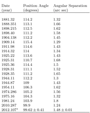
WASP-85 is listed as a known binary in the Washing-ton Double Star catalogue (WDS). We obtained the full set of WDS measurements for the system, which stretch back to 1881. We also measured the position angle and angular separation of the companion star through careful analysis of EulerCAM observations taken on 2012 Febru-ary 7th.
In Figure 7 we show both the binary angular separa-tion and the binary posisepara-tion angle as a funcsepara-tion of cal-endar date. The change in binary separation appears to be roughly periodic, with a period of approximately 30 years. However without error bars for the WDS data, it is likely that this is just random scatter. More high precision measurements of the separation will be needed to determine whether this variation is real; the upcoming GAIA mission will be of great help in this.
The position angle of the binary shows a clear, long-term, decreasing trend. This is a clear indication of orbital motion for the binary, and suggests an orbital period of & 3000 years. This change of position angle suggests that the planet is misaligned from the plane of the binary. Using the distance listed in Table 3, the mean separation of 1.5′′corresponds to a distance be-tween the stars of 186 AU. Using the masses that we es-timate for the two components from our spectral anal-ysis, and assuming a circular orbit, this indicates a pe-riod of 1828 years, far less than the 3000 years suggested by the position angle change. The reverse transforma-tion, from Pbinary = 3000 years, gives a binary distance of 259 AU; again, this is discrepant with the separation derived value. This mismatch suggest that the binary or-bit is inclined relative to our line of sight by ≈ 45◦, again indicating a misalignment with the planet’s orbital plane. The presence of the binary companion at < 259 AU from the planet host star suggests that the protoplane-tary disc was likely truncated, limiting the quantity of material available for planet formation. Exploring this possibility is beyond the scope of this paper, but could be an interesting subject for future work.
Table 7
Position angles and angular separations for the binary star BD+07◦2474 (WASP-85 A B). The majority of the measurements
were obtained from the Washington Double Star catalogue. The most recent datum (marked with∗) was obtained through
analysis of images from EulerCAM, taken on 2012 February 7th. Date Position Angle Angular Separation
(year) (degrees) (arc sec)
1881.32 114.2 1.32 1888.351 113.1 1.66 1898.215 112.5 1.62 1898.40 111.2 1.58 1904.138 112.2 1.45 1909.14 115.4 1.29 1911.98 114.6 1.43 1914.32 114 1.34 1925.22 113.6 1.43 1925.31 110.7 1.68 1925.36 114.4 1.5 1928.31 111.1 1.52 1928.35 111.2 1.65 1944.11 112.2 1.3 1944.87 109 1.43 1954.11 106.3 1.62 1974.286 105.2 1.56 1975.16 104.3 1.32 1981.24 103.9 1.8 2010.287 99.9 1.24 2012.107∗ 99.62 ± 0.41 1.48 ± 0.01
4.3. Highly active stars
Comparing the Ca ii H+K indices for the two stars to the sample of Jenkins et al. (2006, 2008, 2011), we find that both stars fall within the ‘very active stars’ region of Figure 4 in Jenkins et al. (2006). This is con-firmed by Figure 10 of Jenkins et al. (2008) and Figure 6 of Jenkins et al. (2011), where in both cases the two stars fall within the secondary, ‘active’ peak in the log(R′
hk) distribution. Comparison to the sample of Henry et al. (1996) shows that both stars fall in the ‘active’ class of stars.
Comparing to the sample of planet hosting stars exam-ined by Knutson et al. (2010), we see that WASP-85 A is more active than all but one of the stars considered. Only CoRoT-2 is more active. It may be that we have simply observed the system at the peak of the activity cycle, leading to an apparently greater level of activity. However, if we consider the solar cycle then the typi-cal variation is ≈ 0.2 dex; converting the solar Ca ii H+K values presented in Livingston et al. (2007) indicates val-ues of log(R′
hk) = −4.978 and −4.803 at solar minimum and maximum, respectively. Measurements of activity during the Maunder Minimum (Donahue & Bookbinder 1998) indicate log(R′
hk) = −5.102 during that particu-larly inactive period in the Sun’s life, giving a pessimistic variation from maximum of ∼ 0.3 dex. If we apply this to WASP-85 A, then even at stellar ‘minimum’ it will be more active than the Sun at solar maximum, and will still be classified in the ‘active’ class of Henry et al. (1996). It therefore seems that these stars are unusually active for solar-type stars.
The amplitude of rotational variability in K-dwarfs can reach a few percent for periods ∼ 15 days
Figure 7. Upper panel: Angular separation of the two binary components as a function of calendar date. There appears to be short term variation with a period of approximately 30 years. The minimum separation implies an orbital distance of ∼ 150 AU. Lower panel: Binary position angle as a function of calendar date. There is a clear, long-term trend for decreasing position angle. This suggests an orbital period for the binary of & 3000 years. In both panels, black circles indicate data obtained from the Washington Double Star database, while blue triangles indicate data derived from EulerCam observations.
(Collier Cameron et al. 2009). It is therefore possible that the modulation observed in the WASP lightcurve originates from WASP-85 B. The negative correlation that we observe between the HARPS bisector span and RV measurements for WASP-85 B suggest that this might be the case. Though it is fainter, the difference in magnitude is such that the companion contributes signif-icant light (as can be seen from the flux ratio of the two stars). Moreover the projected rotational velocities of the two stars are similar, and both are compatible with the measured rotation period. This degeneracy could be broken by careful, high resolution photometry of the two stars to check their individual rotation periods, or by measurement of the stellar inclinations. If either star is significantly inclined relative to the line of sight, then its true rotation period would be significantly shorter, and thus incompatible with the period determined from the WASP photometry.
4.4. K2 observations
During our campaign of follow-up observations of WASP-85 A b, a search of the proposed K2 fields revealed that the planetary system was visible in the Campaign 1 field. We proposed short cadence observations of WASP-85 under K2 proposal GO1041, and the system was se-lected for observation by K2. Four other K2 Campaign 1 proposals (GO1032, GO1054, GO1059, and GO1005) that included WASP-85 were also selected, three for long cadence observations and one for short cadence observa-tions of the double star.
On the release of the Campaign 1 data, we down-loaded the long cadence data for WASP-85 (short ca-dence data were not immediately available), extracted the photometric data, and corrected it for the system-atic effect of pointing drift. This has been identified as the greatest source of error in the K2 lightcurves (Vanderburg & Johnson 2014). Our detrending method is similar to that developed by Vanderburg & Johnson, and has been previously described in Armstrong et al. (2014). Briefly, we use the centroid positions to create a 2D surface of raw flux as a function of the centroid’s position on the CCD. We then bin this data evenly by both row and column, and linearly interpolate the me-dian flux from each bin to create a variability map. We divide the raw photometry by this surface map to create a corrected flux measurement that is decor related from the spacecraft’s pointing.
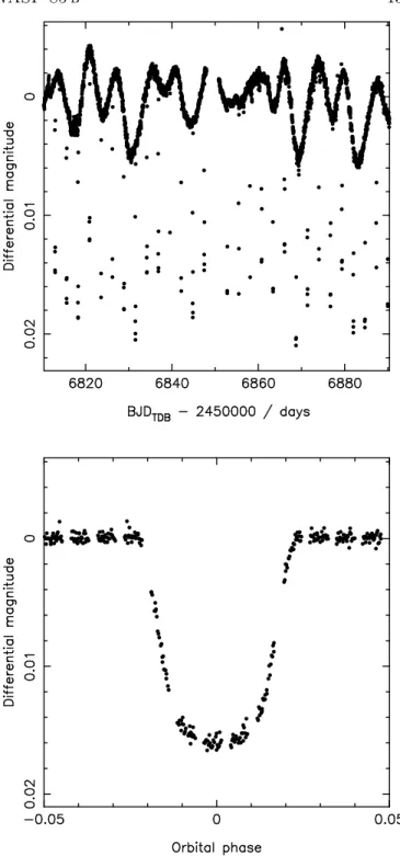
The upper panel of Figure 8 shows the detrended flux as a function of time. The planetary transits are clearly visible where they extend below the stellar lightcurve. Also apparent is the signature of stellar activity; the vari-ations caused by the activity of one or both components of WASP-85 A B appears to be aperiodic at first glance, but this may result from star spot evolution. An ini-tial Lomb-Scargle periodogram analysis of the lightcurve implies a period of 6.66 days for the variability, roughly commensurate with half of the rotation period deter-mined from the WASP data.
The amplitude of the activity signal is approximately half the transit depth. The lower panel of Figure 8 shows the detrended K2 data phase folded on the best fit ephemeris from Table 6. We show only a small win-dow around phase 0 to focus on the planetary transit, and have corrected for the stellar activity using a sim-ple median filter with a window size of 1/100 times the length of the time series. This simple correction for ac-tivity leads to slightly increased scatter between contact points two and three of the transit.
The transit depth is approximately 0.016 magnitudes, less than the transit depth listed in Table 6. This is to be expected given the large pixel scale of the Kepler space-craft’s CCD, which means that the stellar components of the system will be blended together as was the case for our other photometry. The depth discrepancy is as ex-pected given the Kepler passband, the peak transmission of which roughly coincides with the peak transmission of the Johnson R filter (Rowe et al. 2009).
Analysis of the K2 data is ongoing, and incorporates both the long cadence data presented here and the short cadence data that was also collected by K2. The results of this analysis will be presented in a follow-up paper.
5. SUMMARY
We have presented the discovery of WASP-85 A b, a hot Jupiter planet orbiting the brighter component of BD+07◦2474 every 2.66 days. The planet has a mass of Mp = 1.09 ± 0.03 MJup and a radius of Rp = 1.44 ± 0.02 RJup. The host star is similar to the Sun, but has super-solar metallicity, while the companion is a cooler K-dwarf of similar magnitude. The Ca ii H+K activity indices for the two stars indicate that both are strongly active, particularly when compared to other hot Jupiter hosts.
Our photometric observations of WASP-85 are
con-Figure 8. Upper panel: K2 long cadence photometry of BD+07◦2474. The planetary transit signatures are clearly visible,
as is variation arising from stellar activity. This stellar activity sig-nal is of lower amplitude than the planetary transits. The system was also observed in short cadence mode as part of K2 Campaign 1, under our proposal GO1041; this data was not available at time of publication. Lower panel: The K2 long cadence lightcurve, phase folded on the best fit ephemeris from Table 6. We show a small window around phase 0 to focus on the planetary transit. Stellar activity has been corrected for using a simple median filter. Uncertainties are plotted in both panels, but are smaller than the size of the data points.
tain light from both binary components, necessitating the addition of a third light component to the dard transit model, and the modification of our stan-dard WASP analysis routines. Spectroscopic observa-tions with CORALIE and SOPHIE are also diluted by the companion, so we use only radial velocity data ob-tained with HARPS to perform our modelling. We find that the primary effect of the dilution is to decrease the radial velocity semi-amplitude for the affected datasets. If we fail to account for the contamination of the photom-etry, the derived planet radius decreases by 18 percent.
The binary position angle shows a clear, long-term, negative trend that suggests an orbit of & 3000 years. This is at odds with the period derived from the mean binary angular separation, indicating that the binary is likely inclined relative to our line of sight by ≈ 45◦. The planet’s orbit is therefore misaligned with the bi-nary plane.
BD+07◦2474 has been observed at short cadence as part of K2 campaign 1. We have presented the K2 long cadence lightcurve for the system, which clearly shows the variability resulting from stellar activity, with the planetary transits superposed. K2 is unable to distin-guish the binary components. Analysis of this new data is ongoing, and will be presented in a follow-up paper.
My thanks go to Dr. Simon Walker for helpful discus-sions during the analysis process.
The WASP Consortium consists of representatives from the Universities of Keele, Leicester, The Open Uni-versity, Queens University Belfast and St Andrews, along with the Isaac Newton Group (La Palma) and the Insti-tuto de Astrofisica de Canarias (Tenerife). WASP-South is hosted by the SAAO and SuperWASP-North by the Isaac Newton Group and the Instituto de Astrofisica de Canarias; we gratefully acknowledge their ongoing sup-port and assistance. The SuperWASP and WASP-S cam-eras are operated with funds made available from Consor-tium Universities and the STFC. TRAPPIST is funded by the Belgian Fund for Scientific Research (Fond Na-tional de la Recherche Scientifique, FNRS) under the grant FRFC 2.5.594.09.F, with the participation of the Swiss National Science Foundation (SNF). The Liver-pool Telescope is operated on the island of La Palma by Liverpool John Moores University in the Spanish Ob-servatorio del Roque de los Muchachos of the Instituto de Astrofisica de Canarias with financial support from the UK Science and Technology Facilities Council. FC. M. G. and E. J. are FNRS Research Associates. L. D. is an FNRS/FRIA Doctoral Fellow. AHMJT is a Swiss National Science Foundation fellow under grant number P300P2-147773. This research has made use of NASA’s Astrophysics Data System Bibliographic Services, the ArXiv preprint service hosted by Cornell University, the Washington Double Star Catalog maintained at the U.S. Naval Observatory, and the VizieR catalogue access tool, CDS, Strasbourg, France. The original description of the VizieR service was published in A&AS 143, 23.
Facilities: SuperWASP, Euler1.2, Liverpool:2m, ESO:3.6m, OHP:1.93m
REFERENCES Abt H. A., Levy S. G., 1976, ApJS, 30, 273
Alonso R. et al., 2004, ApJ, 613, L153
Anderson D. R. et al., 2012, MNRAS, 422, 1988 Anderson D. R. et al., 2014, MNRAS, 445, 1114 Armstrong D. J. et al., 2014, arXiv:1411.6830
Asplund, M., Grevesse, N., Sauval, A.J., & Scott, P., 2009, ARA&A, 47, 481
Baglin A. et al., 2006, in ‘36th COSPAR Scientific Assembly’, 3749
Bakos G. ´A., L´az´ar J., Papp I., S´ari P., Green E. M., 2002, PASP, 114, 974
Barnes S. A., 2010, ApJ, 722, 222
Barnes S. A., Kim Y.-C., 2010, ApJ, 721, 675 Beatty T. G. et al., 2012, ApJ, 756, L39 Borucki W. J. et al., 2010, Science, 327, 977 Bouchy F. et al., 2009, A&A, 505, 853
Bouchy F., D´ıaz R. F., H´ebrard G., Arnold L., Boisse I., Delfosse X., Perruchot S., Santerne A., 2013, A&A, 549, A49
Brown D. J. A. et al., 2012, ApJ, 760, 139 Brown D. J. A., 2014, MNRAS, 442, 1844 Buchhave L. A. et al., 2011, ApJS, 197, 3
Charbonneau D., Brown T. M., Latham D. W., Mayor M., 2000, ApJ, 529, L45
Claret A., 2000, A&A, 363, 1081 Claret A., 2004, A&A, 428, 1001
Collier Cameron A. et al., 2007, MNRAS, 380, 1230 Collier Cameron A. et al., 2009, MNRAS, 400, 451
Demarque P., Woo J.-H., Kim Y.-C., Yi S. K., 2004, ApJS, 155, 667
‘Cool Stars, Stellar Systems and the Sun’, 1998, Astronomical Society of the Pacific Conference Series, 154, eds. Donahue R. A., Bookbinder J. A.
Dotter A., Chaboyer B., Jevremovi´c D., Kostov V., Baron E., Ferguson J. W., 2008, ApJS, 178, 89
Doyle, A.P., Smalley, B., Maxted, P.F.L., et al., 2013, MNRAS, 428, 3164
Doyle, A.P., Davies, G.R., Smalley, B., Chaplin, W.J., Elsworth, Y., 2014, MNRAS, 444, 3592
Duquennoy A., Mayor M., 1991, A&A, 248, 485
Eastman J., Siverd R., Gaudi B. S., 2010, PASP 122, 935 Gao S., Liu C., Zhang X., Justham S., Deng L., Yang M., 2014,
ApJ, 788, L37
Girardi L. et al., 2010, ApJ, 724, 1030
Gray D.F., 2008, ‘The observation and analysis of stellar photospheres’, 3rd Edition (Cambridge University Press), p. 507.
Henry T. J., Soderblom D. R., Donahue R. A., Baliunas S. L., 1996, AJ, 111, 439
Howell S. B. et al., 2014, PASP, 126, 398 Jehin E. et al., 2011, The Messenger, 145, 2 Jenkins J. S. et al., 2006, MNRAS, 372, 163
Jenkins J. S., Jones H. R. A., Pavlenko Y., Pinfield D. J., Barnes J. R., Lyubchik Y., 2008, A&A, 485, 571
Jenkins J. S. et al., 2011, A&A, 531, A8
Knutson H. A., Howard A. W., Isaacson H., 2010, ApJ, 720, 1569 Lendl M. et al., 2012, A&A, 544, A72
Livingston W., Wallace L., White O. R., Giampapa M. S., 2007, ApJ, 657, 1137
Lucy L. B., Sweeney M. A., 1971, AJ, 76, 544 Magain P., 1984, A&A, 134, 189
Marigo P., Girardi L., Bressan A., Groenewegen M. A. T., Silva L., Granato G. L., 2008, A&A, 482, 883
Mamajek E. E., Hillenbrand L. A., 2008, ApJ, 687, 1264 Mandel K., Agol E., 2002, ApJ, 580, L171
Maxted P. F. L. et al., 2011, PASP, 123, 547 Maxted P. F. L. et al., 2013, PASP, 125, 48
Maxted P. F. L., Serenelli A. M., Southworth J., 2014, arXiv:1412.7891
McCullough P. R., Stys J. E., Valenti J. A., Fleming S. W., Janes K. A., Heasley J. N., 2005, PASP, 117, 783
Neveu-VanMalle M. et al., 2014, A&A, 572, A49
Noyes R. W., Hartmann L. W., Baliunas S. L., Duncan D. K., Vaughan A. H., 1984, ApJ, 279, 763
Pepper J. et al., 2007, PASP, 119, 923
Perruchot S. et al., 2008, in in ‘Society of Photo-Optical Instrumentation Engineers (SPIE) Conference Series’, 7014 Pollacco D. L. et al., 2006, PASP, 118, 1407
Press W. H., Rybicki G. B., 1989, ApJ, 338, 277
Queloz D., Mayor M., Naef D., Santos N., Udry S., Burnet M., Confino B., 2000, in Bergeron J., Renzini A., eds, The VLT Opening Symposium: From Extrasolar Planets to Cosmology, Springer-Verlag, Berlin, p. 548
Queloz D. et al., 2001, A&A, 379, 279 Raghavan D. et al., 2010, ApJS, 190, 1
Roell T., Neuh¨auser R., Seifahrt A., Mugrauer M., 2012, A&A, 542, A92
Rowe J. F. et al., 2009, in ‘Transiting Planets’, Proceedings of IAU Symposium 253, eds.. Pont F., Sasselov D., Holman M. J., p. 121
Santerne A., Moutou C., Bouchy F., 2011, in ‘The astrophysics of planetary systems: formation, structure, and dynamical evolution’, Proceedings of IAU Symposium 276, eds. Sozzetti A., Lattanzi M. G., Boss A. P., p. 549
Schwarz G. E., 1978, Annals of Statistics, 6, 461
Serenelli A. M., Bergemann M., Ruchti G., Casagrande L., 2013, MNRAS, 429, 3645
Sestito, P. & Randlich, S., 2005, A&A, 442, 615 Southworth J., 2010, MNRAS, 408, 1689 Southworth, J., 2011, MNRAS, 417, 2166
Sozzetti A., Torres G., Charbonneau D., Latham D. W., Holman M. J., Winn J. N., Laird J. B., O’Donovan F. T., 2007, ApJ, 664, 1190
Steele I. A. et al., 2004, in ‘Society of Photo-Optical
Instrumentation Engineers (SPIE) Conference Series’, 5489 Torres G., Andersen J. and Gim´enez A., 2010, A&A Rev., 18, 67 Vanderburg A., Johnson J. A., 2014, PASP, 126, 948
Wang J., Fischer D. A., Xie J.-W., Ciardi D. R., 2014, ApJ, 791, 111
Weiss A., Schlattl H., 2008 ,Ap&SS, 316, 99 Wilson D. M. et al., 2008, ApJ, 675, L113 Zechmeister M., K¨urster M., 2009, A&A, 496, 577