Multi-scale Modeling: from Electromagnetism to Grid

(1)

T

H

_H

È

_È

S

_S

E

_E

En vue de l'obtention du

D

O

C

T

O

R

A

T

D

E

L

’

U

N

I

V

E

R

S

I

T

É

D

E

T

O

U

L

O

U

S

E

Délivré par l'INPT - ENSEEIHT (Ecole Nationale Supérieure d'Electrotechnique, d'Electronique,

d'Informatique, d'Hydraulique et des Telecommunications)

Discipline ou spécialité : Micro-ondes Electro-Magnétisme Opto-électronique (MEMO)

JURY

M. Hervé Aubert, M. Fabio Coccetti M. Renaud Loison, M. Christian Perez

M. Michel Daydé, Président M. Yves denneulin, examinateur M. Thierry Monteil, examinateur

M. Luciano Tarricone, invité M. Petr Lorenz, invité

Ecole doctorale : Génie Electrique, Electronique, Télécommunications (GEET)

Unité de recherche : Laboratoire d’Analyse et d’Architecture des Systèmes (LAAS -- CNRS) Directeur(s) de Thèse : M. Hervé Aubert et M. Fabio Coccetti

Rapporteurs : M. Renaud Loison et M. Christian Perez Présentée et soutenue par Fadi KHALIL

Le 14 Décembre 2009

Titre : Modélisation Multi-échelles : de l'Electromagnétisme à la Grille (Multi-scale Modeling: from Electromagnetism to Grid)

(2)

UNIVERSITY OF TOULOUSE

Doctoral School GEET

GENIE ELECTRIQUE ELECTRONQIUE

TELECOMMUNICATIONS

P H D T H E S I S

to obtain the title of

PhD of Science

of INPT - ENSEEIHT

Specialty : MicroOndes, ElectroMagnétisme et

Optoélectronique (MEMO)

Defended on December 14, 2009 by

Fadi KHALIL

Multi-scale Modeling : from

Electromagnetism to Grid

Thesis Advisors : Hervé Aubert and Fabio Coccetti

prepared at the Laboratory of Analysis and Architecture of

Systems (LAAS – CNRS, UPR 8001), MINC Team

Jury :

Reviewers : _{Renaud Loison} - IETR-INSA Rennes

Christian Perez - LIP-ENS Lyon

Members : _{Hervé Aubert} - University of Toulouse, LAAS, INPT-ENSEEIHT Fabio Coccetti - University of Toulouse, Novamems, LAAS

Michel Daydé - University of Toulouse, IRIT, INPT-ENSEEIHT

Yves Denneulin - LIG-ENSIMAG Monbonnot

Thierry Monteil - University of Toulouse, INSA, LAAS, IRIT

Invited : _{Petr Lorenz} - Lorenz Solutions Luciano Tarricone - University of Lecce

(3)

(4)

Acknowledgments

First and foremost, to my thesis advisors, Prof. Hervé Aubert, and Dr. Fabio Coccetti, for supporting this research and for providing an excellent working envi-ronment, for dedicated help, inspiration and encouragement throughout my PhD, for providing sound advice and lots of good ideas, and for good company within and outside the laboratory.

My appreciation goes to my other committee members as well : Prof. Renaud Loison, and Prof. Christian Perez, for having accepted to examine this work and for having provided valuable insights and contributed to the improvement of the quality of this thesis. Thanks are also due to Prof. Michel Daydé for chairing my thesis committee, Prof. Yves Denneulin and Prof. Thierry Monteil.

I appreciate very much the presence, as member of committee, of Prof. Luciano Tarricone and Dr. Petr Lorenz.

My gratitude to Prof. Robert Plana for all of his guidance, assistance, and subtle sense of humor.

I would like to acknowledge the National Research Agency (ANR) for support of MEG Project (ANR-06-BLAN-0006, 2006-2009), and the collaboration of Carlos-Jaime Barrios-Hernandez, and Luis Melo from LIG Laboratory - ENSIMAG.

I firmly believe that the work environment makes the greater part of the learning experience and for this I would like to thank my colleagues in the Laboratory of Architecture and Analysis of Systems. Thank you especially to Bernard Miegemolle, Rémi Sharrock, and Tom Guérout from MRS research group.

My thanks also to Aamir Rashid and Euloge Budet Tchikaya for having provided me with the Scale-Changing Technique modeling codes used in this thesis on Grid platform. I have had three office mates, Jinyu (jason) Ruan, Badreddine Ouagague and Ali Kara Omar, all of them have freely shared their time, opinions and expertise. In addition to my office mates, I would like to extend my gratitude to all MINC research group members for their generous company.

I am grateful to the secretary Mrs. Brigitte Ducroq for helping the lab to run smoothly and for assisting me in many different ways.

Out with the work setting, I would like to offer my fondest regards to my friends : Phélomène Makhraz, Youssef El Rayess, Dalal Boutros, Joseph Chemaly, Georges Khalil, Wissam Karam, Serge Karboyan, Issam Tawk, Florence Freyss, Nancy Nehme, Rania Azar, Micheline Abbas and Hikmat Achkar.

Finally, I would like to mention my family. I wish to thank my parents who raised me, supported me, taught me, and loved me. Many Thanks to my love Nadine Makhraz. To them all I dedicate this thesis.

(5)

(6)

Multi-scale Modeling : from Electromagnetism to Grid

Abstract :The numerical electromagnetic tools for complex structures simulation, i.e. multi-scale, are often limited by available computation resources. Nowadays, Grid computing has emerged as an important new field, based on shared distributed computing resources of Universities and laboratories.

Using these shared resources, this study is focusing on grid computing potential for electromagnetic simulation of multi-scale structure. Since the numerical simula-tions tools codes are not initially written for distributed environment, the first step consists to adapt and deploy them in Grid computing environment. A performance study is then realized in order to evaluate the efficiency of execution on the test-bed infrastructure.

New approaches for distributing the electromagnetic computations on the grid are presented and validated. These approaches allow a very remarkable simulation time reduction for multi-scale structures and friendly-user interfaces.

Keywords : computational electromagnetics, Transmission Line Matrix (TLM), Scale Changing Technique (SCT), Grid computing, distributed computing, performance

(7)

Modélisation Multi-échelles : de l’électromagnétisme à la Grille Résumé : Les performances des outils numériques de simulation électromagné-tique de structures complexes, i.e., échelles multiples, sont souvent limitées par les ressources informatiques disponibles. De nombreux méso-centres, fermes et grilles de calcul, se créent actuellement sur les campus universitaires.

Utilisant ces ressources informatiques mutualisées, ce travail de thèse s’attache à évaluer les potentialités du concept de grille de calcul (Grid Computing) pour la simulation électromagnétique de structures multi-échelles. Les outils numériques de simulation électromagnétique n’étant pas conçus pour être utilisés dans un en-vironnement distribué, la première étape consistait donc à les modifier afin de les déployer sur une grille de calcul. Une analyse approfondie a ensuite été menée pour évaluer les performances des outils de simulation ainsi déployés sur l’infrastructure informatique.

Des nouvelles approches pour le calcul électromagnétique distribué avec ces outils sont présentées et validées. En particulier, ces approches permettent la réalisation de simulation électromagnétique de structures à échelles multiples en un temps record et avec une souplesse d’utilisation.

Mots Clés :modélisation électromagnétique, modélisation par lignes de trans-mission (TLM), modélisation par changements d’échelles (SCT), grille de calcul, calcul distribué, performance

(8)

1 Introduction 1

1.1 Numerical Techniques in CEM . . . 1

1.2 Objectives and Contribution presented in this Thesis . . . 4

1.3 Organization of the Thesis . . . 6

2 Grid Computing 9 2.1 What is the Grid ? . . . 9

2.2 Grids Projects and Applications Area . . . 11

2.3 Grid’5000 . . . 13

2.3.1 Testbed Description . . . 13

2.3.2 Grid’5000 Experimental Activities . . . 15

2.3.3 Cluster Definition . . . 15

2.3.4 Software and Middleware . . . 16

2.3.5 Grid View . . . 16

2.3.6 Typical use case . . . 17

2.3.7 Deploying an Environment . . . 19

2.4 Terminology . . . 20

2.5 Conclusion . . . 24

3 TLM Modeling Method in Grid Environment 27 3.1 Overview of the Transmission Line Matrix (TLM) Modeling Method 27 3.2 From the Huygens principle to TLM modeling . . . 28

3.3 TLM Basics . . . 29

3.4 TLM Algorithm . . . 29

3.5 Implementation of TLM in Parallel computers . . . 32

3.6 Distributed Parallel TLM Simulations in Grid Environment . . . 34

3.6.1 Message Passing Interface (MPI) . . . 35

3.6.2 MPI on Computing Grids . . . 35

3.6.3 Efficiency of using MPI for TLM . . . 37

3.7 Distributed Parametric TLM Simulations in Grid Environment . . . 42

3.7.1 First Approach : Shell Scripts + YATPAC . . . 43

3.7.2 Second Approach : TUNe + YATPAC . . . 49

3.7.3 Third Approach : TUNe + emGine environment . . . 66

4 SCT Modeling Method in Grid Environment 71 4.1 Overview of the SCT Modeling Method . . . 71

4.2 Distributed Parallel SCT Simulations in Grid Environment . . . 74

4.2.1 Optimization of SCT Computing Codes . . . 74

4.2.2 SCT Algorithm . . . 75

1.1 Numerical Techniques in CEM

Modern microwave and radio frequency (RF) engineering is an exciting and dy-namic field, due in large part to the symbiosis between recent advances in modern electronic device technology and the current explosion in demand for voice, data, and video communication capacity. Prior to this revolution in communications, microwave technology was the nearly exclusive domain of the defense industry ; the recent and dramatic increase in demand for communication systems for such applications as wireless paging, mobile telephony, broadcast video, and computer networks is revolutionizing the industry. These systems are being employed across a broad range of environments including corporate offices, industrial and manufac-turing facilities, and infrastructure for municipalities, as well as private homes.

Electromagnetic analysis, a discipline whereby one solves Maxwell’s equations [1] - [3] to obtain better understanding of a complex system, is a critical part of the microwave design cycle. One reason is that Maxwell’s theory is essential for the manipulation of electricity and hence is indispensable. Another reason is that Maxwell’s theory has proven to have strong predictive power. This strong predictive power, together with the advent of computer technology, has changed the practice of electrical engineering in recent years. A complete solution to Maxwell’s equations can expedite many electrical engineering design properties.

Electromagnetic analysis methods can be classified by analytical, semi-analytical and numerical methods. Closed-form solutions in terms of analytical functions can only be found for a few special geometries (for example in rectangular, elliptical, and spherical waveguides and resonators). In spite of their limited practical applicability, analytical solutions are extremely useful for the purpose of validating numerical methods since they provide error-free reference solutions.

Semi-analytical methods were developed before the advent of powerful compu-ters. They involve extensive analytical processing of a field problem resulting in

Chapter 1 Introduction

(11)

2 Chapitre 1. Introduction

a complicated integral, an infinite series, a variational formula, an asymptotic ap-proximation, in short, an expression that requires a final computational treatment to yield a quantitative solution. The analytical preprocessing often leads to rather fast and efficient computer algorithms, but the resulting programs are necessarily specialized since specific types of boundary and material conditions have been in-corporated in the formulation.

Several real-world electromagnetic problems like scattering, radiation, wavegui-ding etc, are not analytically calculable, for the multitude of irregular geometries designed and used. The inability to derive closed form solutions of Maxwell’s equa-tions under various constitutive relaequa-tions of media, and boundary condiequa-tions, is overcome by computational numerical techniques. Numerical methods transform the continuous integral or differential equations of Maxwell into an approximate discrete formulation that requires either the inversion of a large matrix or an ite-rative procedure. There exist many ways to discretize an electromagnetic problem, ranging from very problem- specific to very general purpose approaches.

This makes computational electromagnetics (CEM), an important field in the design, and modeling of antenna, radar, satellite and other such communication systems, nanophotonic devices and high speed silicon electronics, medical imaging, cell-phone antenna design, among other applications (see Figure 1.1).

Figure 1.1 – Impact of Electromagnetics.

Computer-based analysis is at the core of modern simulation tools, and it has revolutionized engineering design, even more so in microwave engineering where these tools allow us to "see" the electromagnetic field and its effects such as current and charge distributions. It reflects the general trend in science and engineering to

(12)

1.1. Numerical Techniques in CEM 3

formulate laws of nature as computer algorithms and to simulate physical processes on digitals computers.

Classification

The purpose of all numerical methods in electromagnetics is to find approxi-mate solutions to Maxwell’s equations (or of equations derived from them) that satisfy given boundary and initial conditions, formulating an electromagnetic pro-blem amounts to specifying the properties that a solution must have in order to qualify. These properties can be specified as local (differential) or global (integral) properties, both in the field space and its boundaries.

When discussing the properties of the different methods, it is necessary to clas-sify them. A major point of difference is the domain they are working in, which is either time domain (TD) or frequency domain (FD). The perceived differences between these two categories are better captured by the terms time-harmonic and transient methods. However, in the formal sense, frequency domain formulations are time domain formulations in which the time dimension has been subject to a Fourier transform, thus reducing the number of independent variables by one. Expressed in a simplistic way, frequency domain formulations are obtained by replacing the time differential operator d/dt by jw, and the time integration operator by −j/w, thus effectively transforming a time differentiation into a multiplication, and a time integration into a division by jw.

Another way of categorizing both the numerical techniques and the computer tools based on them relies on the number of independent space variables upon which the field and source functions depend. In all categories we can again distinguish between frequency domain and time domain formulations.

• 1D Methods : These are methods for solving problems where the field and source functions depend on one space dimension only. Typical applications are transmission line problems, uniform plane wave propagation, and sphe-rically or cylindsphe-rically symmetrical problems with only radial dependence. Transmission-line circuit solvers and the SPICE program are well-known examples of 1D solvers.

• 2D Methods : These are methods for solving problems where the field and source functions depend on two space dimensions. Typical applications are crosssection problems in transmission lines and waveguides, TEn0 propagation in rectangular waveguide structures, coaxial TEM problems, and spherical problems depending only on radius and azimuth or radius and elevation.

• 2.5D Methods : These are methods for solving problems where the fields depend on three space dimensions, while their sources (the currents) are mainly confined planes with two space dimensions. Typical examples are

(13)

planar structures such as microstrip circuits, co-planar circuits, patch antennas, and general multilayer structures that contain planar conductor pattern. The predominant solution method for such structures is the method of moments in the space and spectral domains ; however, the method of lines is also suitable for planar and quasi-planar structures.

• 3D Methods : These are methods for solving problems where both the field and source functions depend on three space dimensions. This category comprises all volumetric full-wave general-purpose formulations.

Hybrid formulations combining two or more different numerical techniques have also been developed and implemented for particular applications.

Figure 1.2shows main numerical modeling methods with respect to discretiza-tion category, distinguishing between volumetric discretizadiscretiza-tion methods and surface discretization methods.

Figure 1.2 – Classification of main numerical methods in electromagnetics. As we can see, there is a vast number of numerical methods one can use to solve the electromagnetic problem. However, not every method is suitable for a particular problem.

1.2 Objectives and Contribution presented in this

The-sis

The area of CEM has undergone a vast development in the past years - giving rise to powerful electromagnetic simulation tools and techniques. The goal of all

(14)

1.2. Objectives and Contribution presented in this Thesis 5

these techniques is to determine and predict performances of RF and microwave components, networks and machines in a very accurate and reliable way.

Recent advances in wireless and microwave communication systems (higher ope-ration frequency bands, more compact topologies containing MMICs and MEMS) have increased the necessity of fast and accurate numerical simulation techniques.

The advent of powerful computers and computer systems allows us to analyze some large and complicated structures, with the numerical efficiency and accuracy remaining at the focal point of today’s research interests. The amount of addressable memory for 64-bit machines goes far beyond the memory addressing limit of 32-bit machines. In theory, the emergence of the 64-bit architecture effectively increases the memory ceiling to 264 addresses, equivalent to approximately 17.2 billion gigabytes. However, this addressing capability is a theoretical number. The support of the memory addressing is still limited by the bandwidth of the bus, the operating system and other hardware and software issues. Most 64-bit microprocessors on the market today have an artificial limit on the amount of memory they can address, because physical constraints make it impossible to support the full 16.8 million terabyte capacity.

Most of the modern full-wave CEM techniques require discretization of the whole computational domain. In order to achieve numerically efficient computations with the available computer memory, one must define a finite computational domain enclosing the problem under analysis and rely on the ways to terminate the com-putational domain at the boundaries.

Despite the recent hardware progress, the computational resources of today’s computers seems to be very limited. It is often impossible to model large volumes of space and/or multi-scale structures with high aspect ratio. The limits up to which we are able to solve a problem are set by :

• memory requirements,

• time needed to process the information.

To get a better feeling for what are the memory requirements to solve an elec-tromagnetic problem, let us take a look at the following example. There is given a structure assumed to be perfect electric conductor (PEC) in air and we wish to compute the scattered electromagnetic field. A three-dimensional computatio-nal domain of 2000 × 2000 × 2000 TLM cells requires 6144000000000 bits1 to hold the information about the electromagnetic field. This amount of information means 715.25 GBytes of memory.

Increasing the spatial resolution just twice in every direction results in eight times larger memory requirements. Furthermore, the time needed to process this amount of information is inverse proportional to the speed of information processing. The need for solving the CEM problem for ever increasing meshes leads to the idea of running these applications in Grid environments. The example shows the reasons why we are not able to discretize very large structures. Consequently, to

1. For the modeling of free-space we need 12 variables per TLM cell. We assume a TLM variable to be represented by 64 bits (double precision). For more information, please refer to Chapter3.

(15)

overcome these problems, large scale computer systems, as Grid Computing, must be used.

Grid computing is currently the subject of a lot of research activities world-wide. Most of these activities aim at providing the necessary tools (for dealing with aspects such as administration, security, performance simulation, discovery, scheduling and volatility of resources, etc.) and programming methodologies. Some studies are centred on applications.

In this thesis, a new methodology is presented for conducting complex mul-tiscale numerical electromagnetic simulations. Technologies from several scientific disciplines, including computational electromagnetics, and parallel computing, are combined to form a simulation capability that is both versatile and practical.

In the process of creating this capability, work is accomplished to conduct first a study designed to adapt the electromagnetic solvers to distributed computing, and to provide an assessment of the applicability of Grid Computing to the field of computational electromagnetics.

Two modeling methods which can be useful to be coupled in a hybrid method have been chosen : the Transmission Line Matrix (TLM) modeling method (3D) and the Scale Changing Technique (SCT) modeling method (2.5D). The efficiency of the modern CEM software to analyze complex microwave structures in Grid Com-puting environments are investigated with real life examples. Multiscale strutures, i.e. planar reflectarrays, have been simulated and the radiation patterns plotted. After a performance study, well adapted approaches are proposed and tested on Grid nodes.

In order to keep the use of Grid Computing transparent to electronic engineer that are not probably computer science specialists, friendly solutions as graphical user interfaces (GUI) have been used.

1.3 Organization of the Thesis

The thesis is organized as follows. Chapter 2 introduces the Grid Computing and distributed systems, and a brief overview of Grid applications. Grid’5000, the test-bed platform used to run all the experiments in this thesis, is also presented in a way to show underlying hardware, network and software. This chapter is then concluded by the definition of essential terms used the following chapters.

In Chapter 3, the Transmission Line Matrix (TLM) method is described. The principles of the method are shown as well as the interconnection of TLM nodes and their contributions in the algorithm. A quick overview of past works on pa-rallel TLM shows different approaches that have been used. Then, both proposed approaches (distributed parallel and parametric TLM computing) are investigated and perfomance evaluated. Simulations of a coplanar phase-shifter based on MEMS and reflectarrays are shown.

Chapter4is devoted to the Scale-Changing Technique (SCT) modeling method. The distribution of the independant tasks are described in detail. Reflectarrays are

(16)

1.3. Organization of the Thesis 7

simulated in parallel on Grid’5000 nodes. Parametric analysis, for frequency sweep and convergence, shows the efficiency of using large scale Grids.

Finally, the conclusions of the thesis are presented in Chapter 5. Appendix A

and Appendix B describes two electromagnetic tools based on TLM and used in this thesis. The theory used in this thesis to design the array antennas with steered beams is presented in AppendixC. AppendixDlists different acronyms used.

(17)

(18)

Contents

2.1 What is the Grid ? . . . . 9

2.2 Grids Projects and Applications Area . . . . 11

2.3 Grid’5000 . . . . 13

2.3.1 Testbed Description . . . 13

2.3.2 Grid’5000 Experimental Activities . . . 15

2.3.3 Cluster Definition . . . 15

2.3.4 Software and Middleware . . . 16

2.3.5 Grid View . . . 16

2.3.6 Typical use case . . . 17

2.3.7 Deploying an Environment . . . 19

2.4 Terminology . . . . 20

2.5 Conclusion . . . . 24

This chapter provides an overview of Grid Computing, its different applica-tion domains and some related terminology. It presents also the testbed platform, Grid’5000, used along this thesis to run computational electromagnetics experi-ments.

2.1 What is the Grid ?

The popularity of the Internet as well as the availability of powerful computers and high-speed network technologies as low-cost commodity components is changing the way we use computers today. These technology opportunities have led to the possibility of using distributed computers (nodes) as a single, unified computing re-source, leading to what is popularly known as Grid computing (GC) [4] - [9]. Grid Computing has emerged as an important new field, distinguished from conventio-nal distributed computing by its focus on large-scale resource sharing1, innovative applications, and, in some cases, high-performance orientation.

The term "the Grid" was coined in the mid of 1999s2 to denote a proposed distributed computing infrastructure for advanced science and engineering. In 1997, CPU scavenging and volunteer computing were popularized by distributed.net [10]

1. In Grid terms, a resource is any kind of software (a piece of application, a file, a database, etc.) or hardware entity (an electrical device, a storage card, etc.) accessible through the network.

2. The name "Grid Computing" is inspired by the electrical grid.

Chapter 2 Grid Computing

(19)

10 Chapitre 2. Grid Computing

and later in 1999 by SETI@home [11] to harness the power of networked PCs worldwide, in order to solve CPU-intensive research problems.

The ideas of the grid (including those from distributed computing, object-oriented programming and Web services) were brought together by Ian Foster, Carl Kesselman, and Steve Tuecke, widely regarded as the "fathers of the grid" [5] - [9]. They led the effort to create the Globus Toolkit3 incorporating not just computation management but also storage management, security provisioning, data movement, monitoring, and a toolkit for developing additional services based on the same infrastructure, including agreement negotiation, notification mechanisms, trig-ger services, and information aggregation [12]. While the Globus Toolkit remains the de facto standard for building Grid solutions, a number of other tools have been built that answer some subset of services needed to create an enterprise or global Grid.

Computational Grids may span domains of different dimensions, starting from local Grids, where the nodes belong to a single organization via a LAN connection, to global Grids, where the nodes are owned by different organizations and linked via Internet.

Grid applications (typically multidisciplinary and large-scale processing appli-cations) often couple resources that cannot be replicated at a single site, or which may be globally located for other practical reasons, and belonging to multiple individuals or organizations (known as multiple administrative domains), in a flexible and secured environment. These are some of the driving forces behind the foundation of global Grids. In this light, the Grid allows users to solve larger or new problems by pooling together resources that could not be easily coupled before. Hence, the Grid is not only a computing infrastructure, for large applica-tions, it is a technology that can bond and unify remote and diverse distributed resources ranging from meteorological sensors to data vaults, and from parallel supercomputers to personal digital organizers.

A Grid could be characterized by four main aspects [13] :

• Multiple administrative domains and autonomy. Grid resources are geographically distributed across multiple administrative domains and owned by different organizations. The autonomy of resource owners needs to be honored along with their local resource management and usage policies. • Heterogeneity. A Grid involves a multiplicity of resources that are

hetero-geneous in nature and will encompass a vast range of technologies.

• Scalability. A Grid might grow from a few integrated resources to millions. This raises the problem of potential performance degradation as the size of Grids increases. Consequently, applications that require a large number

(20)

2.2. Grids Projects and Applications Area 11

of geographically located resources must be designed to be latency and bandwidth tolerant.

• Dynamicity or adaptability. In a Grid, resource failure is the rule rather than the exception. In fact, with so many resources in a Grid, the probability of some resource failing is high. Resource managers or applications must tailor their behavior dynamically and use the available resources and services efficiently and effectively.

Over the last decade, an increasing number of scientists have run their workloads on large-scale distributed computing systems such as Grids. The concept of Grid computing started as a project to link geographically dispersed supercomputers, but now it has grown far beyond its original intent. The Grid infrastructure can benefit many applications, including among others collaborative engineering, data exploration, high-throughput computing, and distributed supercomputing.

2.2 Grids Projects and Applications Area

There are currently a large number of international projects and a diverse range of new and emerging Grid developmental approaches being pursued worldwide. These systems range from Grid frameworks to application testbeds, and from collabora-tive environments to batch submission mechanisms (integrated Grid systems, core middleware, user-level middleware, and applications/application driven efforts ...) [14,15].

Grid resources can be used to solve grand challenge problems in areas such as biophysics, chemistry, biology, scientific instrumentation [16], drug design [17,18], tomography [19], high energy physics [20], data mining, financial analysis, nuclear simulations, material science, chemical engineering, environmental studies, climate modeling [21], weather prediction, molecular biology, neuroscience/brain activity analysis [22], structural analysis, mechanical CAD/CAM, and astrophysics.

In the following, two applications of interest to NASA [23] are illustrated. Key aspects of the design of a complete aircraft (airframe, wing, stabilizer, engine, lan-ding gear and human factors) are depicted in Figure 2.1.

Each part could be the responsibility of a distinct, possibly geographically dis-tributed, engineering team whose work is integrated together by a Grid realizing the concept of concurrent engineering. Figure 2.2 depicts possible Grid controlling satellites and the data streaming from them. Shown are a set of Web (OGSA [25]) services for satellite control, data acquisition, analysis, visualization and linkage (assimilation) with simulations as well as two of the Web services broken up into multiple constituent services.

Meanwhile, the community of electromagnetics (EM) research has been only peripherally interested in Grid Computing (GC) until 2004 [26]4_{. Few works in}

(21)

Figure 2.1 – A Grid for aerospace engineering showing linkage of geographically separated subsystems needed by an aircraft [24].

Figure 2.2 – A possible Grid for satellite operation showing both spacecraft ope-ration and data analysis. The system is built from Web services (WS) and it shows how data analysis and simulation services are composed from smaller WS’s [24].

electromagnetics could be found.

(22)

tea-2.3. Grid’5000 13

med with Hewlett-Packard, BAE SYSTEMS and the Institute of High Performance Computing in Singapore, to use Grid computing for the exploration of advanced, collaborative simulation and visualization in aerospace and defense design [27].

One year after, Lumerical launches parallel FDTD solutions on the supercom-puting infrastructure of WestGrid in Canada [28], even though their field of interest is more in optical and quantum devices rather than in RF applications.

Another recent example of distributed computing using a code based on the TLM (Transmission Line Matrix, defined in chapter 3) method has been demons-trated in Germany [29].

In 2006, computer scientists from different french labs started the DiscoGrid project [30]. It aims at studying and promoting a new paradigm for programming non-embarrassingly parallel scientific computing applications on distributed, he-terogeneous, computing platforms. The target applications require the numerical resolution of systems of partial differential equations (PDEs) for computational electromagnetism (CEM) [31] and computational fluid dynamics (CFD).

In [32], EM researchers can identify new and promising Information and Com-munication Technologies (ICT) tools (already available, or to be consolidated in the immediate future), expected to significantly improve their daily EM investigation.

Later, a Web-based, Grid-enabled environment for wideband code-division multiple-access (WCDMA) system simulations, based on Monte Carlo methods, has been implemented and evaluated on the production Grid infrastructure deployed by the Enabling Grids for E-sciencE (EGEE) project [33].

2.3 Grid’5000

2.3.1 Testbed Description

Grid’5000 [34] is a research effort developing a large scale nationwide infrastructure for large scale parallel and distributed computing research5. It aims at providing a highly reconfigurable, controllable and monitorable experimental platform to its users [35]. The initial aim (circa 2003) was to reach 5000 processors in the platform. It has been reframed at 5000 cores, and was reached during winter 2008-2009. For the 2008-2012 period, engineers of ADT ALADDIN-G5K initiative are ensuring the development and day to day support of the infrastructure.

The infrastructure of Grid’5000, which is a Multi-clusters Grid, is geographically distributed on different sites hosting the instrument, initially 9 in France (17 Labo-ratories). The current plans are to extend from the 9 initial sites each with 100 to a thousand PCs, connected with a 10Gb/s link by the RENATER (v5) Education and Research Network [36] to a bigger platform including a few sites outside France not necessarily connected through a dedicated network connection. Porto Alegre, in Brazil, is now officially becoming the 10th site and Luxembourg should join shortly.

5. Other testbeds for experiments : PLANETLAB (http ://www.planet-lab.org/), Emulab (http ://www.emulab.net/), DAS-3 (http ://www.starplane.org/das3/), GENIE (http ://www.genie.ac.uk/)

(23)

Figure2.3 shows the Grid’5000 backbone connecting the nine sites of this Grid (Bordeaux, Grenoble, Lille, Lyon, Nancy, Orsay, Rennes, Sophia and Toulouse). Each site is composed of a heterogeneous set of nodes and local networks (High performance networks : Infiniband 10G (161 cards), Myrinet 2000 (222 cards), My-rinet 10G (423 cards), Gigabit Ethernet 1 or 10 Gb/s). The "standard" architecture is based on 10Gbit/s dark fibers and provides IP transit connectivity, intercon-nection with GEANT-2 [37], overseas territories and the SFINX (Global Internet exchange).

Figure 2.3 – Grid’5000 Backbone.

Grid’5000 clusters have been built mainly upon 64 bits bi-processors architec-tures (AMD Opteron (78%) and Intel Xeon EMT64 (22%)), but a certain degree of (desired) heterogeneity appears from cluster to cluster6. The user of this architec-ture can choose the CPU family in order to run its own experiments, which could be MonoCore (41%), DualCore (46%), QuadCore (13%). All computing nodes have local disks (generally 80 gigabytes IDE or SATA) that are all partitioned the same way (for all clusters at all sites). The frontends (Figure2.5) generally feature huge storage space (0.5 or 1 terabyte) mainly for the home directories (note that these homes are in general not backuped nor synchronized from cluster to cluster).

(24)

2.3. Grid’5000 15

2.3.2 Grid’5000 Experimental Activities

This platform is used for large research applicability Grid experiments7 (see Figure

2.4) to address critical issues of Grid system/middleware (Programming, scalabi-lity, fault tolerance, scheduling), of Grid networking (High performance transport protocols, QoS), to gridify and test real life applications and investigate original mechanisms (P2P resources discovery, desktop Grids).

Figure 2.4 – Grid’5000 Applications.

2.3.3 Cluster Definition

All computers from a given site (a geographical place where a set of computing resources shares the same administration policy), which are connected to a given network architecture, define a cluster. Every cluster basically consists of :

• one (or more) frontend machine(s), that serve(s) as resource allocation plat-form(s), so that each user may request usage of whole or part of the other nodes ;

– some of these frontends are accessible from the public internet domain, generally through a firewall, depending on local security policies ;

• the computing nodes themselves that form the main cluster, the main com-puting power ; each node may have several CPUs (and each CPU possibly several cores) ; depending on the resource manager middleware configuration, it is possible to request resource allocation at the node level or at the CPU level ;

7. A summary of the domains of experiment which Grid’5000 is providing a research platform for can be found on https ://www.grid5000.fr/mediawiki/index.php/Grid5000 :Experiments.

(25)

• for security and/or redundancy reasons, there may be servers besides the frontends to isolate critical software and services ;

– in principle, servers and frontends do not take part to the computing power of the cluster and therefore are not counted as computing nodes in the cluster hardware description ;

• the network architecture onto which all nodes, frontends and servers are phy-sically connected ; it is in principle isolated from the public internet domain (private IP addresses), but is interlinked with the other sites through a privi-leged RENATER network.

2.3.4 Software and Middleware

The middleware is the software suite that performs the main tasks during computing nodes usage. It mainly consists of a resource allocation manager involving :

• node(s) reservation for a given user and a given duration (with possible envi-ronment customization) ;

• task(s) scheduling over reserved nodes (with possible results retrieval) ; • resource deallocation after tasks completed to make them available again for

new tasks.

In the case of Grid’50008, job scheduling and resource allocation and dealloca-tion is performed by OAR [38] at the cluster level.

Grid’5000 has also made the choice to allow users to customize their environ-ment and even install their own preferred operating system on the reserved nodes. This implies some preliminary work to build this kind of customized environment. It is generally a hard work, but allows for optimum experiment conditions and reproductability (as long as the hardware does not change).

However, a default Linux environment is available in case of experiments that do not need customization. The KaTools (kadeploy, karun, kaenvironments, karecor-denv) [39] have been designed in this purpose of custom environment deployment. 2.3.5 Grid View

The Grid architecture for Grid’5000 is achieved by the privileged interlinks existing between the different clusters, using the local network architecture for clusters at a given site, or provided by RENATER from site to site.

The Grid middleware layer consists of tools able to request resource allocation on several clusters at the same time, using a simple synchronization mechanism to associate what are basically separate resources. The privileged links between sites formerly used 10 gigabit optic fibers technology (RENATER v5 network) dedicated only to the Grid’5000 traffic.

To briefly summarize the common general security policy overall Grid’5000 net-work, it is allowed to perform SSH connections inbound frontends (and not

el-8. Software mainly developed in Grid’5000 and available for its users : https ://www.grid5000.fr/mediawiki/index.php/Grid5000 :Software

(26)

2.3. Grid’5000 17

sewhere) and outbound nowhere. In other words, intrusions are allowed through narrow one-way windows, but the huge computing power from Grid’5000 may not be used to attack any server on the public internet side (also known as the out-side)... Local policies may differ about the inbound connections from the outside. Internal connections from one site to another are completely free, either inbound or outbound nodes as well as frontends.

The main internal network services (DNS directories for the machines, LDAP directories for the users’ accounts...) are common and distributed among all sites across this dedicated internal network (private IP addresses). External network services (WiKi website, email lists manager...) are centralized on dedicated hosts belonging to the outside (public IP addresses).

2.3.6 Typical use case

An experiment could be resumed in following six steps : 1. Connect to the platform on a site

2. Reserve some resources

3. Configure the resources (optional) 4. Run experiment

5. Grab the results 6. Free the resources

A Grid’5000 Experiment Workflow is sketched in Figure 2.6. In fact, when en-tering a site, user is connected to its access frontend (Figure2.5). Thus he is not on its submission frontend. Some sites possess only one frontend to do external access and job submission, but this is not the case everywhere and other sites possess one frontend for external access and another one for job submission.

On each Grid’5000 site, user possesses a Grid-independent home directory. Thus before submitting jobs over the Grid, user must be sure that code and configura-tion are available on each used cluster. SSH publickey and configuraconfigura-tion must be synchronized.

OAR [38] is the resource manager (or batch scheduler for large clusters) used to manage Grid’5000 platform’s resources which support KADEPLOY [39]. It allows cluster users to submit or reserve nodes either in an interactive or a batch mode.

(27)

Figure 2.5 – Grid’5000 access and job submissions.

OAR is an open source batch scheduler which provides a simple and flexible exploitation of a cluster. It manages resources of clusters as a traditional batch scheduler9. It is flexible enough to be suitable for production clusters and research experiments. It currently manages all the Grid’5000 nodes and has executed millions of jobs. When making a reservation, one specifies which nodes to use. Nodes can be chosen by the user, or automatically selected.

Note that for Grid experiment, a really simple tool named OARGRID was built upon OAR to help you using distant resources. OARGRID is a Grid version of OAR. It provides the capability of globally reserving nodes on the whole Grid’5000 platform (several sites at once). Oargridsub perform an OAR reservation on each specified clusters. An identity number is given by OARGRID, so with it all reser-vation information could be found. It returns a Grid job id to bind cluster jobs together if the inherent cluster reservations succeed. If one of them did not succeed then all previous reservations are canceled and also the global operation.

The reservations and submissions could be monitored by graphical tools Current and scheduled jobs could be displayed by Monika [40] or by oarstat, a command-line tool to view current or planned job submission (running or waiting). oarnodes is also

9. as PBS (http ://www.pbsgridworks.com/), Torque (http ://www.clusterresources.com/products/torque-resource-manager.php), LSF (http ://www.platform.com/products/LSF/), SGE (http

(28)

2.3. Grid’5000 19

Figure 2.6 – Grid’5000 Experiment Workflow.

a command-line tool. It shows cluster node properties (list states and informations of all nodes). Among returned information there is current node state. This state is generally free, job or Absent. When nodes are sick, their state is Suspected or Dead.

DrawOARGantt displays past, current and scheduled OAR jobs, while Ganglia [41] provides resources usage metrics (memory, cpu, jobs...) for individual sites or the whole Grid.

To analyze standard output stdout and standard error output stderr of the main node, where script is run, OAR puts theses output in files named OAR.scriptname.IdJ ob.stdname.

In order to show who is using the platform, as well as the Number of usage hour (per month per cluster or per month per site), Kaspied is a statistic tool provided. Nagios [42] monitors critical Grid servers and services and automatically reports incidents and failures.

Note that while using above mentioned tools, user can choose individual site or cluster, or have a global view of the Grid.

2.3.7 Deploying an Environment

As mentioned in previous sections, KADEPLOY is the deployment system which is used by Grid’5000. It is a fast and scalable deployment system towards cluster and Grid computing. It provides a set of tools, for cloning, configure (post installation) and manage a set of nodes. Currently it deploys successfully Linux, *BSD, Windows, Solaris on x86 and 64 bits computers.

(29)

Any user may deploy his own environment (see Figure2.6), which actually means any OS adapted by him to suit his experiments needs, on his reserved computational nodes10. This way, he has a full control over which software or library is used, what kind of kernel or OS is running and how the system is configured for instance. Each site maintains an environment library in the /grid5000/images directory of the OAR node. To deploy an environment, by using a simple command kaenvironments on the frontend, user can know its name as registered in the KADEPLOY database.

2.4 Terminology

In order to have a clearer understanding of the upcoming discussion, the following terminology is introduced :

Virtual Organization

In grid computing, a Virtual Organization (VO) is a set of users working on similar topics and whose resources requirements are quite comparable. The users usually share their resources between them (data, software, CPU, storage space). The collaborations involved in Grid computing lead to the emergence of multiple organizations that function as one unit through the use of their shared competencies and resources for the purpose of one or more identified goals.

A user needs to be a member of a VO before he is allowed to submit jobs to the Grid. Moreover, a VO is usually defined by a name, and a scope which represents a geographical location constraint.

Grid Application

A Grid application is a collection of work items to solve a certain problem or to achieve desired results using a Grid infrastructure. For example, a Grid application can be the simulation of electromagnetic structure, like a planar antenna, that require a large amount of data as well as a high demand for computing resources in order to calculate and handle the large number of variables and their effects. For each set of parameters a complex calculation can be executed. The simulation of a large scale scenario then consists of a larger number of such steps. In other words, a Grid application may consist of a number of jobs that together fulfill the whole task.

Job

A job is considered as a single unit of work within a Grid application. It is typically submitted for execution on the Grid, has defined input and output data, and execution requirements in order to complete its task. A single job can launch

10. In this thesis, a customized environment called MEG, including an OS in addition to some needed libraries and legacy files, is used to run TLM and SCT experiments. (see Chapter3and4)

(30)

2.4. Terminology 21

one or many processes on a specified node. It can perform complex calculations on large amounts of data or might be relatively simple in nature.

Parallel computing

The simultaneous execution of the same task (split up and specially adapted) on multiple processors in order to obtain results faster. The idea is based on the fact that the process of solving a problem usually can be divided into smaller tasks (see Figure2.7), which may be carried out simultaneously with some coordination.

Figure 2.7 – Parallel application flow.

To take advantage of parallel execution in a Grid, it is important to analyze tasks within an application to determine whether they can be broken down into individual and atomic units of work that can be run as individual jobs.

Serial or sequential Computing

In contrast to the parallel flow is the serial application flow. In this case there is a single thread of job execution where each of the subsequent jobs has to wait for its predecessor to end (see Figure 2.8) and deliver output data as input to the next job. This means any job is a consumer of its predecessor, the data producer.

Figure 2.8 – Serial job flow.

In this case, the advantages of running in a Grid environment are not based on access to multiple systems in parallel, but rather on the ability to use any of several

(31)

appropriate and available resources. Note that each job does not necessarily have to run on the same resource, so if a particular job requires specialized resources that can be accommodated, while the other jobs may run on more standard and inexpensive resources.

Parametric Computing

An application may consist of a large number of such calculations where the start parameters are taken from a discrete set of values. Each resulting serial application flow then could be launched in parallel on a Grid in order to utilize more resources. The serial flow A through D in Figure 2.8 is then replicated to A’ through D’, A" through D", and so forth.

Distributed computing

Distributed computing is a field of computer science that studies distributed systems, which consist of multiple autonomous computers (with onboard CPU, sto-rage, power supply, network interface, etc.) that communicate through a computer network. This is in contrast to the traditional notion of a supercomputer, which has many processors connected by a local high-speed computer bus.

The computers interact with each other in order to achieve a common goal. A computer program that runs in a distributed system is called a distributed program, and distributed programming is the process of writing such programs.

Distributed computing also refers to the use of distributed systems to solve computational problems. In distributed computing, a problem is divided into many tasks, each of which is solved by one computer.

Speedup

There are always parts of a program that cannot run in parallel, where code must run in serial. In parallel computing, speedup refers to how much a parallel algorithm is faster than a corresponding sequential algorithm.

The serial parts of the program cannot be speedup by concurrency. Let p be the fraction of the program’s code that can be made parallel (p is always a fraction less than 1.0). The remaining fraction (1-p) of the code must run in serial. In practical cases, p ranges from 0.2 to 0.99.

The potential speedup for a program is proportional to p divided by the CPUs applied, plus the remaining serial part, 1-p.

As an equation, Amdahl’s law could be expressed as : Speedup(N ) = _p 1

N + (1 − p)

(2.1) The maximum possible speedup (if applying an infinite number of CPUs) would

(32)

2.4. Terminology 23

be 1/(1-p). The fraction p has a strong effect on the possible speedup.

When the value of p could not be defined for a given problem, the following equation could be used :

Speedup(N ) = T s TN

(2.2) where N is the number of processors, T s is the execution time of the sequential algorithm and T_N is the execution time of the parallel algorithm with N processors. Linear speedup or ideal speedup is obtained when Speedup(N ) = N . When running an algorithm with linear speedup, doubling the number of processors doubles the speed. As this is ideal, it is considered very good scalability.

Granularity

Granularity is a measure of the size of the components (the size of the units of code under consideration in some context), or descriptions of components, that make up a system. Systems of, or description in terms of, large components are called coarse-grained, and systems of small components are called fine-grained. In parallel computing, granularity means the amount of computation in relation to communication, i.e., the ratio of computation to the amount of communication.

Fine-grained, or "tightly coupled, parallelism" means individual tasks are

re-latively small in terms of code size and execution time. The data are transferred among processors frequently in small amounts of messages.

Coarse-grained, or loosely coupled, is the opposite : data are communicated

infrequently, after larger amounts of computation. Execution Time

The execution time of a parallel program is defined here as the time that elapses from when the first processor starts executing on the problem to when the last processor completes execution, while one job is assigned to one processor.

During execution, each processor is computing or communicating. The computa-tion time of an algorithm (Ticomp) is the time spent performing computation rather than communicating, while the communication time of an algorithm (Ticomm) is the time that its tasks spend sending and receiving messages.

On the ith processor, Ti = Ticomp + Ticomm.

Hence, to determine the total computation and communication performed by a parallel algorithm rather than the time spent computing and communicating on in-dividual processors, total execution time T can be defined as the biggest value of Ti: T = max (i=[0, N-1])(Ticomp + Ticomm), while N is the number of processors

(33)

Both computation and communication times are specified explicitly in a parallel algorithm ; hence, it is generally straightforward to determine their contribution to execution time.

On the Grid, two distinct types of nodes communication will be distinguished : internodes communication and intranode communication. In internodes communi-cation, two communicating tasks are located on different Grid nodes. This will be the case of distributed computing. In intranode communication, two communicating tasks are located on the same Grid node (via local bus).

Note that only the internodes communication will be highlighted later in the Grid experiments. This kind of communication could be established between nodes from the same cluster, called intracluster communication (i.e. two nodes of Pastel cluster in Grid’5000 Toulouse site), nodes from different clusters but in the same Grid site, called intrasite communication (i.e. one node of Pastel cluster and one node of Violette cluster in Grid’5000 Toulouse site), or nodes belonging to geographically remote sites, called intersite communication (i.e. one node from Toulouse site and another from Bordeaux site).

Bandwidth and Latency

Bandwidth in computer networking refers to the data rate (overall capacity of the connection ) supported by a network connection or interface. The greater the capacity, the more likely that better performance will result.

Network bandwidth is not the only factor that contributes to the perceived speed of a network. A lesser known but other key element of network performance - latency - also plays an important role.

Latency could be defined as the delay between the initiation of a network trans-mission by a sender and the receipt of that transtrans-mission by a receiver. In a two-way communication, it may be measured as the time from the transmission of a re-quest for a message, to the time when the message is successfully received by the requester.

The basic formula used to estimate communication time is T comm = L + s/B, where T comm is the elapsed time to finish the communication, L is the latency of the network between the sender and the receiver, s is the size of the message and B is the available bandwidth.

2.5 Conclusion

Grid computing offers a model for solving computational problems by making use of resources (CPU cycles and/or disk storage) of large numbers of disparate com-puters, treated as a virtual cluster embedded in a distributed telecommunications infrastructure. Grid computing’s focus on the ability to support computation across administrative domains sets it apart from traditional computer clusters or traditio-nal distributed computing. This approach offers a way to solve Grand Challenge

(34)

2.5. Conclusion 25

problems like protein folding, financial modelling, earthquake simulation, and cli-mate/weather modeling.

But the use the Grid means dealing with aspects such as performance simulation, scheduling and volatility of resources, etc. An application that runs on a stand-alone computer must be "gridified" before it can run on a Grid. In this work, the Grid is used to run electromagnetic simulations of complex structures. Modeling methods will be deployed on Grid’5000 nodes and the performance will be evaluated.

(35)

(36)

Contents

3.1 Overview of the Transmission Line Matrix (TLM) Mode-ling Method . . . . 27 3.2 From the Huygens principle to TLM modeling . . . . 28 3.3 TLM Basics . . . . 29 3.4 TLM Algorithm . . . . 29 3.5 Implementation of TLM in Parallel computers . . . . 32 3.6 Distributed Parallel TLM Simulations in Grid Environment 34

3.6.1 Message Passing Interface (MPI) . . . 35 3.6.2 MPI on Computing Grids . . . 35 3.6.3 Efficiency of using MPI for TLM . . . 37

3.7 Distributed Parametric TLM Simulations in Grid Environ-ment . . . . 42

3.7.1 First Approach : Shell Scripts + YATPAC . . . 43 3.7.2 Second Approach : TUNe + YATPAC . . . 49 3.7.3 Third Approach : TUNe + emGine environment . . . 66

3.8 Conclusion . . . . 69

The Transmission Line Matrix (TLM) method, a flexible method used to model arbitrary and complex electromagnetic structures, is introduced in this chapter. The "gridification" of this method is then discussed and experiments presented.

3.1 Overview of the Transmission Line Matrix (TLM)

Modeling Method

The TLM method is a key numerical method in computational electromagnetics. It is based on the equivalence between Maxwell’s equations and the equations for voltages and currents on a mesh of continuous two-wire transmission lines.

This method is based on the analogy between the electromagnetic field and a mesh of transmission lines [43]. As a network model of Maxwell’s equations for-mulated in terms of the scattering of impulses, it possesses exceptional versatility, numerical stability, robustness and isotropic wave properties.

Chapter 3 TLM Modeling Method in Grid

Environment

(37)

28 Chapitre 3. TLM Modeling Method in Grid Environment

The main feature of this method is the simplicity of formulation and program-ming for a wide range of applications [44,45]. As compared to the lumped network model, the transmission line model is more general and performs better at high fre-quencies where transmission and reflection properties of geometrical discontinuities cannot be regarded as lumped [46].

The TLM was originally used for modeling electromagnetic wave propagation [44], [47], [48] but since it is based on Huygens principle it could be used for modeling any phenomena which obeys this principle. Researchers showed that TLM can be used to solve the following problems : Diffusion problem [49], Vibration [50], Heat transfer [51], Radar [52], Electromagnetic compatibility [53].

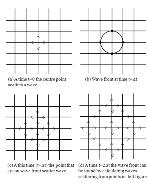
Figure 3.1 – Huygens Principle.

3.2 From the Huygens principle to TLM modeling

Two distinct models describing the phenomenon of light were developed in the seventeenth century : the corpuscular model by Isaac Newton and the wave model by Christian Huygens. At the time of their conception, these models were considered incompatible. However, modern quantum physics has demonstrated that light in particular, and electromagnetic (EM) radiation in general, posses both granular (photon) and wave properties. These aspects are complementary, and one or the other dominates, depending on the phenomenon under study.

(38)

3.3. TLM Basics 29

TLM modeling is based on the Huygens principle which is [54] - [56] :

All points on a wave front serve as point sources of spherical secondary wavelets. After a time T the new position of the wave front

will be the surface of tangency to these secondary wavelets

This principle is shown in Fig 3.1. At time 0 the central point scatters a wave. The wave front at time t1 is shown in Figure3.1(b). At this time (time = t1 ) we can assume that all points on the wave front are acting as a point sources (shown in Figure3.1(c)) and the wave front at any time later ( for example t2 ) is the wave front from these secondary point sources (Figure3.1(d)).

In order to implement Huygens’s model on a digital computer, one must formu-late it in discretized form.

3.3 TLM Basics

Johns and Beurle [47] modeled this principle in 1971 by sampling the space and representing it with a mesh of passive transmission line components. The wave propagation was modeled as voltage and current travelling in this mesh. Time was also sampled and the relationship between ∆t, the sample interval and ∆l, the sample space, is :

∆l = ∆t.c where c is the wave speed in the medium.

In Figure 3.2 wave propagation in a two dimensional TLM mesh is shown. Assume that at time zero, an impulse is incident to the middle node (Figure3.2(a)). This node scatters the wave to its 4 neighboring nodes. The scattered wave reaches the neighboring nodes at time = ∆t (Figure 3.2(b)). Now these 4 nodes scatter waves to their neighboring nodes (Figure3.2(c)). At time = 2∆t the wave front can be found by finding waves scattered from points in Figure3.2(b) as shown in Fiure

3.2(d). At each time step, each node receives an incident wave from its neighbors and scatters it to its neighbors. By repeating the above calculation for each node, the wave distribution on the medium can be calculated. Subsequent papers by Johns and Akhtarzad [57] - [63] extended the method to three dimensions and included the effect of dielectric loading and losses. Building upon the groundwork laid by these original authors, other researchers [64] - [87] added various features and improvements such as variable mesh size, simplified nodes, error correction techniques, and extension to anisotropic media.

3.4 TLM Algorithm

As explained above, the TLM method, like other numerical techniques, is a discre-tization process. Unlike other methods such as finite difference and finite element

(39)

Figure 3.2 – Wave propagation in a two dimensional TLM mesh.

methods, which are mathematical discretization approaches, the TLM is a physical discretization approach.

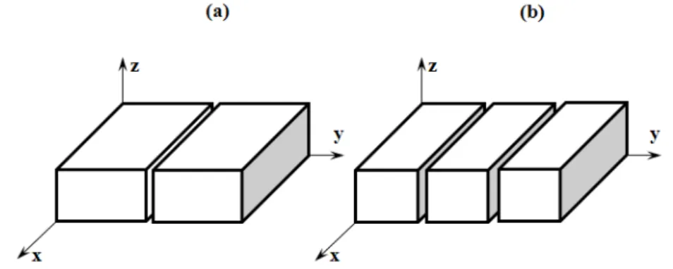
For example, consider the structure to simulate in Figure3.3. The TLM method involves dividing the solution region into a rectangular mesh of transmission lines. Junctions are formed where the lines cross forming the impedance discontinuities.

A comparison between the transmission line equations and Maxwell’s equations allows equivalences to be drawn between voltages and currents on the lines and electromagnetic fields in the solution region.

When all sections of a medium have the same properties, the medium is referred as homogeneous. For modeling homogeneous media it does not need to consider the medium properties and hence it is possible to use the simple mesh.

The relationship between the incident wave (voltage in transmission line) and the scattered wave is :

(40)

3.4. TLM Algorithm 31

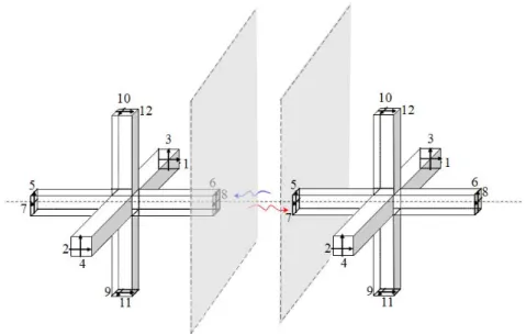
Figure 3.3 – Entire space is discretized. On each face of each cell (cuboïd) the field is decomposed in the two polarization components (i stand for incident, s stands for scattered). The cubic cell is modeled by the three-dimensional symmetrical conden-sed (SCN) TLM node propoconden-sed by P. B. Johns in 1986.

V_ks = S . Vi

k; Vk+1i = C . Vks

In this figure, Vi represents the incident wave (voltage in the transmission line) and Vs represents the scattered wave. S is the impulsive scattering matrix of the node, and C is a connection matrix describing the topology of the TLM mesh. k and k+1 are arbitrary consecutive time steps separated by the sample interval ∆t. Based on this equation, if the magnitude of the wave (voltage in the TLM modeling) is known at any time k. ∆t then the magnitude of wave in the mesh could be found at time (k+1). ∆t. By repeating this for each time step, wave propagation could be modeled.

In the case of square cell (uniform mesh) and loss-free propagation wave, the scattering matrix S is a 12x12 sparse matrix.

When modeling a non homogeneous medium, one should consider the properties of the medium in the model. For this reason a new model for a node is created by adding a capacity [57], [58]. This model is valid when the medium is lossless. When there are some losses in the medium, there is a resistor in parallel to the capacitor to model the loss [61].

In case of non uniform mesh (cell with ∆x 6= ∆y 6= ∆z) where stub are introduced to compensate line delay in the scattering, the resulting is a scattering matrix S of 18x18. If it is completely equipped with permittivity, permeability,

(41)

and loss stubs, the matrix goes up to 30x30.

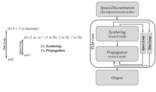
Thus, the TLM method involves two basic steps [88] :

- Replacing the field problem by the equivalent network and deriving the analogy between the field and network quantities.

- Solving the equivalent network by iterative methods.

Figure 3.4 – TLM Algorithm.

3.5 Implementation of TLM in Parallel computers

Since TLM is a numerical model, it should be implemented in software and executed in digital computers. Since TLM requires that the entire computational domain be gridded, and the grid spatial discretization must be sufficiently fine to resolve both the smallest electromagnetic wavelength and the smallest geometrical feature in the model, very large computational domains can be developed, which results in very long solution times (which is also the case of the Finite-difference time-domain (FDTD)). Thus it needs a large amount of memory and CPU power to model wave propagation, and consequently it is hard to model a real wave propagation problem with normal computers.

Since the TLM algorithm is based on local operations at neighboring mesh nodes only, the TLM method seems to be adapted for parallel computing. Clearly, to have a single processor working though the computations for each node in turn is therefore a suboptimal solution. Furthermore, since a speed increase is required, parallel processing is a logical step even if the communication is a critical point.

There are a number of different models of parallelism that has been conside-red. Past work on parallel TLM has often used special hardware. A number of papers discuss using Transputers (Transistor Computer). In [89], Transputers have