Science Arts & Métiers (SAM)
is an open access repository that collects the work of Arts et Métiers Institute of Technology researchers and makes it freely available over the web where possible.
This is an author-deposited version published in: https://sam.ensam.eu
Handle ID: .http://hdl.handle.net/10985/13556
To cite this version :
Mohamed BEN BETTAIEB, Farid ABED-MERAIM - Localized necking in elastomer-supported metal layers: impact of kinematic hardening Journal of Manufacturing Science and Engineering -Vol. 139, n°6, p.3461-3480 - 2017
Any correspondence concerning this service should be sent to the repository Administrator : archiveouverte@ensam.eu
1
Localized necking in elastomer-supported metal layers: impact of
kinematic hardening
Mohamed Ben Bettaieb*, Farid Abed-Meraim
LEM3, UMR CNRS 7239 – Arts et Métiers ParisTech, 4 rue Augustin Fresnel, 57078 Metz Cedex 3, France
DAMAS, Laboratory of Excellence on Design of Alloy Metals for low-mAss Structures, Université de Lorraine, France
*Correspondence to: Mohamed Ben Bettaieb; E-mail: Mohamed.BenBettaieb@ensam.eu
Abstract
The present paper deals with localized necking in stretched metal sheets using the initial
imperfection approach. The first objective is to study the effect of kinematic hardening on the
formability of a freestanding metal layer. To this end, the behavior of the metal layer is
assumed to follow the rigid-plastic rate-independent flow theory. The isotropic (resp.
kinematic) hardening of this metal is modeled by the Hollomon (resp. Prager) law. A
parametric study is carried out in order to investigate the effect of kinematic hardening on the
formability limits. It is shown that the effect of kinematic hardening on the ductility limit is
noticeably different depending on the strain path considered. The second aim of the paper is
to analyze the effect of an elastomer substrate, perfectly bonded to the metal layer, on the
formability of the whole bilayer. It is found that the addition of an elastomer layer
substantially enhances the formability of the bilayer, in agreement with earlier studies.
Keywords
Prager's model; freestanding metal layer; metal/elastomer bilayer; formability limit; imperfection approach2
Notations, conventions and abbreviations
The derivations presented in this paper are carried out using classic conventions. Note that the
assorted notations can be combined, while additional notations will be clarified as needed
following related equations.
1 Introduction
The accurate prediction of localized necking in thin metal sheets still represents an ambitious
challenge for the design of structural components in many advanced technology applications,
despite the substantial advances and achievements made in this field. The most common
representation of this limit of material formability is through the concept of forming limit
diagram (FLD). Note that this concept was initially introduced in 1960s by Keeler and
Vectorial and tensorial fields are designated by bold letters and symbols Scalar variables and parameters are represented by thin letters and symbols
Einstein’s convention of summation over repeated indices is adopted. The range of the free (resp. dummy) index is given before (resp. after) the corresponding equation
time derivative of T
transpose of tensor
tensor product of two vectors ( i j)
I
value of quantity at the initial time
t
value of quantity at time t (for convenience, the dependence on time is most often omitted when the variable is expressed in the current instant)
( )
quantity associated with behavior in layer B
quantity associated with behavior in the band S
quantity associated with behavior in the safe zone
2
3
Backofen [1] available in the range of positive minor principal strains (i.e., ε20). The previous work was extended later by Goodwin [2] to the range of negative minor principal
strains (i.e., ε20). The FLDs can be determined experimentally or theoretically (e.g., [3–6]). Because the experimental determination of FLDs has proven to be both expensive and
difficult, considerable effort has been expended in prior literature towards the development of
reliable theoretical and/or numerical predictive models. It is well known that the formability
limit of metal sheets is often strongly influenced by the constitutive behavior and the material
parameters of the studied sheet metal [7]. It is demonstrated for example that the ductility
increases with the hardening exponent in the case of power-type isotropic hardening [8]. Also,
the material viscosity plays an important role in the enhancement of the formability of
metallic sheets, as shown in [9] and [10]. The impact of other constitutive features and
phenomena on the formability limit has been widely investigated in the literature. In this
regard, we can quote the studies of Neale and Chater [11], Cao et al. [12] and Kuroda and
Tvergaard [13], aiming at understanding the effect of plastic anisotropy on ductility, as well
as the contributions of Haddag et al. [14] and Mansouri et al. [15], concerning the effect of
damage-induced softening on the prediction of sheet metal formability. The effect of
kinematic hardening on localized necking in biaxially stretched sheets has also been
investigated by Tvergaard [16]. However, this earlier study was restricted to loading paths
corresponding to the range of positive biaxial stretching (i.e., ranging from plane-strain
tension to equibiaxial tension). Also, in that previous investigation, the Ziegler hardening law
was used to model the kinematic hardening. More recent works have been carried out in order
to investigate the impact of kinematic hardening on the ductility limit of sheet metals. In this
regard, we can quote the contribution of He et al. [17], who used the Yoshida–Uemori
two-surface kinematic hardening model to assess the effect of kinematic hardening on the onset of
localized necking in metal sheets subjected to stretch-bending loading. The same kinematic
hardening model has been more recently used in [18] to investigate the effect of nonlinear
strain paths on forming limits of stretched metal sheets. In the present work, the localized
4
hardening law. More specifically, the effect of kinematic hardening (modeled by Prager law)
on localized necking in a freestanding metal layer is investigated for the full range of loading
paths that span the forming limit diagram (FLD) (i.e., ranging from uniaxial tension to
equibiaxial tension).
Due to the theoretically infinite ductility of elastomer materials, bonding an elastomer layer,
as substrate, to a freestanding metal layer allows substantially enhancing the ductility of the
resulting bilayer. This result has been highlighted by several experimental investigations.
However, most commonly conducted experiments are uniaxial tensile tests ([19-21]) or
experiments performed under dynamic conditions ([22]). Therefore, the necking instability in
substrate-supported metal layers under biaxial loading conditions remains poorly understood
so far, and only few theoretical works have been dedicated to this important issue. In this
regard, one can quote Guduru et al. [23], who developed a numerical approach, based on the
linear stability analysis, in order to predict the ductility of multi-layers under dynamic
conditions. Jia and Li [24] used the bifurcation analysis proposed in [25] to numerically
determine the necking limit of substrate-supported metal layers under static in-plane biaxial
loading. More recently, Ben Bettaieb and Abed-Meraim [26] investigated the ductility limits
of substrate-supported metal layers using both the bifurcation analysis and the initial
imperfection approach, initially introduced by Marciniak and Kuczynski [27] and designated
hereafter as M–K. In these earlier numerical contributions ([23], [24], [26]), the mechanical
behavior of the metal layer follows a rigid-plastic rate-independent model, while plasticity
and hardening are assumed to be isotropic. In the current paper, however, the former
investigations carried out in [26] are extended to take into account the description of
kinematic hardening within the metal layer. In contrast to the earlier investigations based on
isotropic hardening models, the current extension allows accurately describing some
important physical phenomena, such as the Bauschinger effect. This effect is commonly
observed in a number of metallic materials, such as dual phase (DP) steels. To evaluate the
ductility of freestanding metal layers and metal/substrate bilayers, the initial imperfection
5
an elastomer substrate can significantly retard the occurrence of localized necking in
metal/elastomer bilayers. This confirms the previous studies made without considering
kinematic hardening in the constitutive modeling. It is also demonstrated, through several
numerical simulations, that kinematic hardening tends to enhance the ductility of the
metal/elastomer bilayer.
The reminder of the paper is organized as follows:
Section 2 outlines the constitutive equations, expressed under an Eulerian formulation, which describe the behavior of the metal and elastomer layers.
Section 3 details the imperfection approach adopted to predict localized necking in the bilayer. For convenience, Lagrangian formulation is employed to develop the main
equations governing this approach.
Section 4 deals with the algorithmic aspects relating to the powerful numerical tool developed for the prediction of localized necking.
The various numerical predictions are presented in Section 5, where the effects on localized necking of kinematic hardening and of the addition of an elastomer layer are
discussed in details.
2 Constitutive equations
2.1 Metal layerThe constitutive behavior of the metal layer is assumed to be incompressible, rigid-plastic and
obeying the flow theory of plasticity. Accordingly, the plastic flow is defined by the normality
law p eq F ε ε σ , (1)
where ε is the equivalent strain rate and eq F is the yield function. p The above yield function F is defined by the following expression: p
p Y
6
where:
S denotes the deviatoric part of the Cauchy stress tensor σ ,
X is the back-stress tensor, which describes the yield surface translation,
Y
σ is the yield stress, which measures the evolution of the size of the yield surface. The isotropic hardening is assumed to follow the Hollomon law [28]
nY eq
σ ε . (3)
For the kinematic hardening, the rate of the back-stress tensor X is assumed to be
proportional to the strain rate tensor ε, as described by the following linear Prager model [29]:
C
X ε . (4)
The scalars , n, and C introduced in Eqs. (3) and (4) denote material parameters. 2.2 Elastomer layer
The constitutive behavior of an elastomer substrate is described by a neo-Hookean model [30]
2 2
q ; μ
σ I B B V , (5)
where μ is the shear modulus, q is an unknown pressure to be determined by the incompressibility constraint, and V is the left Cauchy-Green tensor defined by the following relation:
2 T
V FF , (6)
with
F
being the deformation gradient tensor.The constitutive framework, developed in Section 2, will be integrated in Section 3 into the
equations governing the imperfection approach in order to develop a numerical tool able to
7
3 Imperfection approach
3.1 Governing equations for the imperfection approach
The prediction of localized necking in thin substrate-supported metal layers is carried out
using the initial imperfection approach, which was originally developed by Marciniak and
Kuczynski [27] and designated hereafter as the M–K approach. The initial imperfection (in
the form of a groove), required for the M–K analysis, is assumed to initiate within the metal
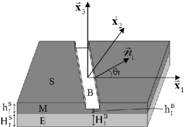
layer. The elastomer layer is assumed to be initially homogeneous. Fig. 1 depicts the
geometry of the bilayer.
Fig. 1 Illustration of the M–K analysis for a bilayer in its initial configuration.
In the sequel, the following notations will be employed:
B
I
h : the initial thickness of the metal layer M inside the band B.
S
I
h : the initial thickness of the metal layer M in the safe zone S.
B
I
H : the initial thickness of the elastomer layer E inside the band B.
S
I
H : the initial thickness of the elastomer layer E in the safe zone S (equal to H ). BI NI: the initial unit normal to the band.
θI: the initial orientation of the band.
The initial imperfection factor ξI is defined by the following relation:
B I I S I h ξ h . (7)
8
The M–K analysis is characterized by the following assumptions and relations:
The two layers are assumed to be perfectly adhered (i.e., no delamination is allowed), which can be expressed as follows:
B B B S S S
(M) (E) ; (M) (E)
F F F F F F , (8)
where FB(M) refers to the deformation gradient in the metal layer located within the band zone.
The kinematic compatibility condition between the band and the safe zone
B S
I
F F C N , (9)
where C is the jump vector that expresses the discontinuity in the strain field between
the band and the safe zone. This jump vector is assumed to be uniform and continuous
at the interface between the two layers.
The equilibrium of the normal and shear forces across the imperfection band is also maintained throughout the deformation
B B
S S
I I
hIBP (M)HIBP (E) .N hSIP (M)HSIP (E) .N , (10) where P is the first Piola–Kirchhoff stress tensor related to σ by
T
J
P σ F . (11)
As the different layers are incompressible, the Jacobian of the deformation gradient J is
equal to 1 all along the deformation for both layers.
The constitutive equations (1)–(4) for the metal layer and (5)–(6) for the elastomer layer, formulated under the plane-stress conditions, as will be detailed in Section 3.2.
In order to predict the FLD, proportional strain paths are prescribed to the safe zone of the
bilayer as follows: S S S S 22 12 13 23 S 11 ε constant ; ε ε ε ε . (12)
9
Exploiting the incompressibility condition of the metal and elastomer layers along with the
plane-stress conditions, and making use of Eq. (12), the strain rate tensor in the safe zone can
be expressed as [26] S 11 S S 11 S 11 ε 0 0 0 ρε 0 0 0 (1 ρ) ε ε . (13)
Then, the expression of the deformation gradient in the safe zone F can be easily derived S from Eq. (13) S 11 S 11 S 11 ε ρε S ρ ε e 0 0 0 e 0 0 0 e F . (14)
Combining the compatibility condition (9) and the particular expression (14) of F , the S deformation gradient in the band can be expressed in the following form:
S 11 S 11 S S S 11 11 11 ε 1 I1 1 I 2 ρε B 2 I1 2 I 2 ρ+1)ε ρε ε 1 I1 2 I 2 e C C 0 C e C 0 1 0 0 e C e C e F N N N N N N . (15)
3.2
Algorithm for the prediction of FLDs
The general algorithm used to predict the FLD of the metal/elastomer bilayer is based on the
10
For ρ 1 2/ to ρ 1 at user-defined intervals (here, we take intervals of 0 1. ).
For θI spanning the admissible range of inclination angles (i.e., between 0 and
90), at user-defined intervals (here, we take intervals of 1).
For each time increment [t , tn nΔt], an implicit incremental algorithm is developed and used to integrate the governing equations of the metal and
elastomer layers in both the safe zone and the band. The application of this
incremental integration scheme is stopped when the following criterion is
reached:
B S
33 33
ε /ε 0. (16)
The strain component ε , thus obtained once the criterion (16) is satisfied, is S11 considered to be the critical strain ε corresponding to the current band *11 inclination θ and strain path ρ .
The smallest critical strain ε , solution of the above algorithm, over all initial angles *11 θI and the corresponding current angle define, respectively, the necking limit strain ε and 11L the necking band orientation for the current strain-path ratio ρ .
4 Results and discussions
This section is divided into two main sections, which correspond respectively to the
freestanding metal layer results and the metal/elastomer bilayer results.
4.1 Freestanding metal layer
In order to investigate the effect of kinematic hardening on the ductility limit of a freestanding
metal layer, a parametric study is conducted in this paper. In this parametric study, four
fictitious materials are considered. For each fictitious material, two sets of parameters are
considered: the first set corresponds to the isotropic hardening model (without kinematic
hardening), while the second is associated with the mixed hardening model (combined
isotropic and kinematic hardening). The parameters (M)
K and (M)
11
mixed hardening model, are kept identical for all materials (as detailed in Table 1), and only
parameter C (of the Prager model) is varied from one material to another (100 MPa, 200 MPa,
300 MPa and 400 MPa). Once the parameters corresponding to the mixed hardening model
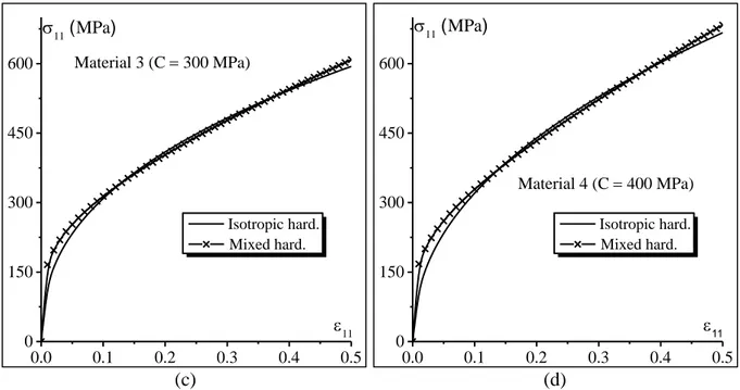
are fixed, the hardening parameters K(I) and n(I) for the isotropic hardening model are fitted in
order to obtain the same uniaxial stressstrain response yielded by the two hardening models for each fictitious material, as shown in Fig. 2. Reference to the metal or elastomer layer is
obviously omitted in this section, as only a freestanding metal layer is studied here.
(a) (b) 0.0 0.1 0.2 0.3 0.4 0.5 0 150 300 450 600 11 Isotropic hard. Mixed hard. 11 (MPa) Material 1 (C 100 MPa) 0.0 0.1 0.2 0.3 0.4 0.5 0 150 300 450 600 Material 2 (C 200 MPa) 11 Isotropic hard. Mixed hard. 11 (MPa)
12
(c) (d)
Fig. 2 Comparison between the stressstrain curves obtained by isotropic hardening and mixed hardening: (a) Material 1 (C 100 MPa ); (b) Material 2 (C200 MPa); (c) Material 3
(C300 MPa); (d) Material 4 (C400 MPa ).
The material parameters corresponding to all materials for both hardening models are given in
Table 1.
Table 1 Hardening parameters
Isotropic hardening Mixed hardening
(I) K [MPa] (I) n K(M) [MPa] (M) n C [MPa] Material 1 553 0.292 447 0.221 100 Material 2 668 0.354 447 0.221 200 Material 3 787 0.406 447 0.221 300 Material 4 914 0.455 447 0.221 400
Before analyzing the effect of kinematic hardening for the whole range of strain paths,
attention is first confined to the particular case of plane-strain state (ρ 0 ). For this strain path, the necking band orientation θI and the normal vector NI are equal to 0° and (1, 0, 0),
0.0 0.1 0.2 0.3 0.4 0.5 0 150 300 450 600 Material 3 (C 300 MPa) 11 Isotropic hard. Mixed hard. 11 (MPa) 0.0 0.1 0.2 0.3 0.4 0.5 0 150 300 450 600 Material 4 (C 400 MPa) 11 Isotropic hard. Mixed hard. 11 (MPa)
13
respectively, as demonstrated by many authors (see, for instance, [8]). Hence, Eq. (10) reduces
to
B S
11 11
h PBI h PSI . (17)
For this particular case, the strain path remains linear during the deformation both in the safe
zone and in the band. The deformation gradient tensors F and S F are expressed as follows: B
S B 11 11 S B 11 11 ε ε S B ε ε e 0 0 e 0 0 0 1 0 ; 0 1 0 0 0 e 0 0 e F F . (18)
By combining Eqs. (11), (17) and (18), one can easily derive the Eulerian form, equivalent to
Eq. (17) B S 11 11 ε B ε S 11 11 h eBI σ h eSI σ . (19)
On the other hand, the expressions of S 11
σ and B 11
σ can be derived by combining the plane-stress conditions and the constitutive equations of the metal layer
n
n n B n S 11 11 B B S S 11 11 n 1 11 11 n 1 2 2 2 K ε 2 K ε σ Cε ; σ Cε 3 3 , (20)where C , K, and n are the hardening parameters. Hence, Eq. (19) can be rewritten as
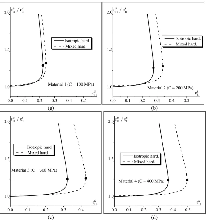
B S 11 11 n n n B n S 11 11 ε B ε S 11 n 1 11 n 1 2 2 2 K ε 2 K ε h e Cε h e Cε 3 3 B S I I . (21)The strain component ε is varied between 0 and 1, with an increment size of 11B 3
10 . For each
value of ε , Eq. (21) is solved iteratively, providing the corresponding value of 11B ε . The 11S evolution of the ratio ε11B/ε11S is plotted in Fig. 3 as a function of ε , for the different 11S materials defined in Table 1. The initial imperfection factor I, which is equal to (hBI h )SI , as stated by Eq. (7), is fixed to 2
10 . The dots tagged on each curve indicate the maximum
14 S
11
ε is reached, the strain rate component S 33
ε (equal to S 11
ε
in this case) becomes very small compared to ε , and criterion (16) is accordingly satisfied. The different curves reported in 33B Fig. 3 indicate that, for this particular plane-strain loading path, the consideration of kinematic
hardening tends to increase the limit strain.
(a) (b)
(c) (d)
Fig. 3 Evolution of the strain ratio ε11B/ε11S as a function of ε for the plane-strain state S11 (freestanding metal layer): (a) Material 1; (b) Material 2; (c) Material 3; (d) Material 4.
0.0 0.1 0.2 0.3 0.4 0.5 1.0 1.5 2.0 Material 1 (C 100 MPa) Isotropic hard. Mixed hard. B S 11 11 ε /ε S 11 ε 0.0 0.1 0.2 0.3 0.4 0.5 1.0 1.5 2.0 Material 2 (C 200 MPa) Isotropic hard. Mixed hard. B S 11 11 ε /ε S 11 ε 0.0 0.1 0.2 0.3 0.4 1.0 1.5 2.0 Material 3 (C 300 MPa) Isotropic hard. Mixed hard. B S 11 11 ε /ε S 11 ε 0.0 0.1 0.2 0.3 0.4 0.5 1.0 1.5 2.0 Material 4 (C 400 MPa) Isotropic hard. Mixed hard. B S 11 11 ε /ε S 11 ε
15
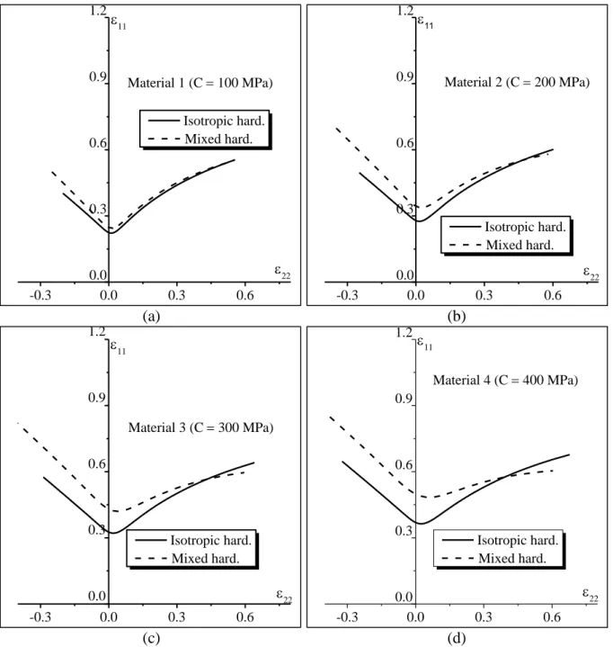
The influence of the kinematic hardening parameter C on the shape and the level of FLDs is
depicted in Fig. 4. In this figure, the initial imperfection factor I (i.e., the initial value for the factor defined in Eq. (7)) is equal to 2
10 . From these different curves, the following
conclusions can be drawn:
Despite the similarity of the uniaxial stress–strain curves given by the two hardening models (isotropic and mixed), as shown in Fig. 2, the level and the shape of the
associated FLDs differ (see Fig. 3). This difference is due to the fact that the strain path
inside the band evolves during the deformation. Indeed, at the beginning of straining,
the components of the jump vector C are very small and, consequently, the deformation
gradient and the strain path inside the band are very close to their counterparts outside
the band (see Eq. (9)). As deformation progresses, the strain path inside the band
gradually deviates from proportionality. Thus, although both hardening models provide
the same uniaxial stress–strain response, they yield different mechanical responses
inside the band (due to the complexity in the loading path). These differences clearly
justify why the predicted limit strains are influenced by the hardening model
considered.
For Material 1, the difference between the FLD predictions corresponding to isotropic and mixed hardening models is relatively small. This is due to the small value of the
kinematic hardening parameter C, which induces a small effect of back-stress.
For the other materials (2, 3 and 4), the effect of kinematic hardening on the limit strain depends on the strain path ρ considered. It is observed that the predicted limit strain is increased for strain paths ranging from 0.5 to 0.5, while it is lowered in the neighborhood of equibiaxial tension (i.e., ρ
0 5 1. , ).
16
(a) (b)
(c) (d)
Fig. 4 Effect of kinematic hardening on the FLDs of freestanding metal layer: (a) Material 1; (b) Material 2; (c) Material 3; (d) Material 4.
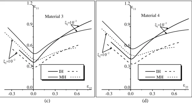
The impact of the initial imperfection factor I on the shape and the level of the FLDs for both hardening models is depicted in Fig. 5. In this figure, two different initial imperfection
factors are considered in the simulations: 103 (curves with solid lines) and 102 (curves with
dashed lines). As well known from several previous works (see, for instance, [8, 26]), the
effect of increasing the initial imperfection is essentially to shift the FLD downwards. Thus,
the level of the FLD decreases when the value of the initial imperfection factor I increases.
-0.3 0.0 0.3 0.6 0.0 0.3 0.6 0.9 1.2 Material 1 (C 100 MPa) 22 11 Isotropic hard. Mixed hard. -0.3 0.0 0.3 0.6 0.0 0.3 0.6 0.9 1.2 Material 2 (C 200 MPa) 22 11 Isotropic hard. Mixed hard. -0.3 0.0 0.3 0.6 0.0 0.3 0.6 0.9 1.2 Material 3 (C 300 MPa) 22 11 Isotropic hard. Mixed hard. -0.3 0.0 0.3 0.6 0.0 0.3 0.6 0.9 1.2 Material 4 (C 400 MPa) 22 11 Isotropic hard. Mixed hard.
17
For both hardening models, the imperfection plays a destabilizing role that precipitates the
occurrence of strain localization. It is also observed from these figures that the impact of the
hardening model on the necking strains is consistently the same, whatever the value of the
initial imperfection factor. In other words, for the two imperfection values I, the limit strain increases with the kinematic hardening parameter C for strain paths ranging from 0.5 to 0.5 , while it decreases in the neighborhood of equibiaxial tension (i.e., ρ
0 5 1. , ). Although
similar trends are observed, it should be noted that the difference between the FLDpredictions yielded by the isotropic and mixed hardening models increases with decreasing
the initial imperfection. For the sake of conciseness, isotropic hardening (resp. mixed
hardening) is referred to as IH (resp. MH) inFig. 5.
(a) (b) -0.3 0.0 0.3 0.6 0.0 0.3 0.6 0.9 1.2 Material 1 22 11 IH MH -0.3 0.0 0.3 0.6 0.0 0.3 0.6 0.9 1.2 Material 2 22 11 IH MH
18
(c) (d)
Fig. 5 Effect of the initial imperfection factor on the FLDs of freestanding metal layer: (a) Material 1; (b) Material 2; (c) Material 3; (d) Material 4.
4.2 Metal/Elastomer bilayer
In this section, a bilayer combination is considered: a metal layer supported by an elastomer
substrate. In all calculations reported in this section, the material parameters of the metal layer
are those given in Table 1. The shear modulus of the elastomer layer is fixed to 22 MPa. This latter choice is based on data for polyurea [31].
Similar to the case of a freestanding metal layer, we first consider the plane-strain case
( ρ0 ). In this case, an analytical formula, comparable to Eq. (21), can be derived after some straightforward developments
B B B 11 11 11 S S S 11 11 11 n n B 11 2 ε 2ε ε B 11 n 1 2 n n S 11 2 ε 2ε ε S 11 n 1 2 2 K ε e 2 h C ε H e e 3 2 K ε e 2 h C ε H e e 3 B B I I S S I I . (22)Again, for each prescribed value of ε , Eq. (22) is solved iteratively to determine the 11B corresponding value of ε . In this process, the prescribed strain component S11 ε is varied 11B
-0.3 0.0 0.3 0.6 0.0 0.3 0.6 0.9 1.2 Material 3 22 11 IH MH -0.3 0.0 0.3 0.6 0.0 0.3 0.6 0.9 1.2 Material 4 22 11 IH MH
19
between 0 and 1. The initial imperfection ratio I is fixed to 2
10 . To emphasize the effect of
the elastomer layer, Fig. 6 compares the evolution of ε11B/ε11S as a function of ε , with and S11 without addition of an elastomer layer, for the different materials defined in Table 1. For the
sake of clarity, only the results corresponding to mixed hardening are reported in Fig. 6. It is
clearly shown from this figure that, for this particular plane-strain loading path, the addition
of an elastomer layer allows enhancing the ductility of the resulting bilayer.
(a) (b) 0.0 0.2 0.4 0.6 0.8 1.0 1.5 2.0 Material 1 (mixed hardening) HI/hI0 HI/hI1 B S 11 11 ε /ε S 11 ε 0.0 0.2 0.4 0.6 0.8 1.0 1.5 2.0 Material 2 (mixed hardening) HI/hI0 HI/hI1 B S 11 11 ε /ε S 11 ε
20
(c) (d)
Fig. 6 Evolution of strain ratio ε11B/εS11 as a function of ε for the plane-strain state S11 (metal/elastomer bilayer): (a) Material 1 (mixed hardening); (b) Material 2 (mixed hardening);
(c) Material 3 (mixed hardening); (d) Material 4 (mixed hardening).
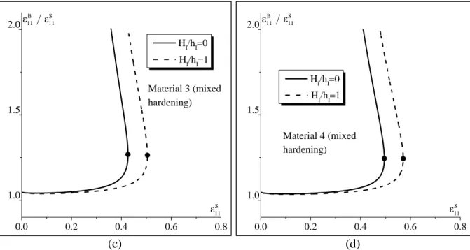
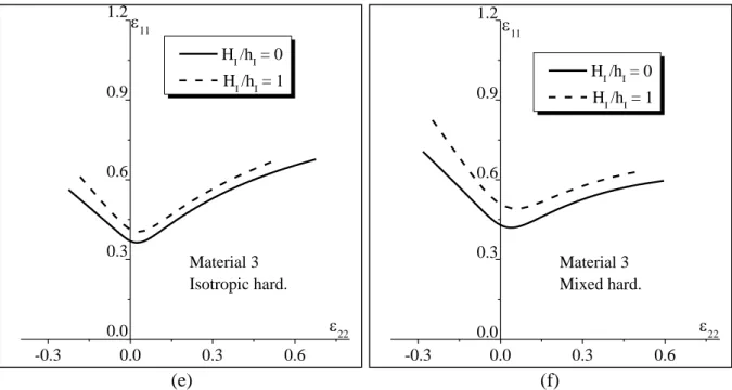
Several simulations are carried out in order to further investigate the effect of the thickness of
the elastomer layer, relative to that of the metal layer, on the ductility of the bilayer. The
results are reported in Fig. 7 for an initial imperfection factor I equal to 2
10 . These
simulations demonstrate that the effect of the substrate layer on the ductility of the bilayer is
quite significant and confirm the previously reported results regarding the positive effect of
the elastomer layer on the necking limit. Fig. 7 shows that the limit strains increase as the
ratio of the initial thicknesses H / hI I increases, revealing that a relatively thicker substrate
leads to more necking retardation. The above results and observations are valid for all
different materials modeled with both hardening descriptions.
0.0 0.2 0.4 0.6 0.8 1.0 1.5 2.0 Material 3 (mixed hardening) HI/hI0 H I/hI1 B S 11 11 ε /ε S 11 ε 0.0 0.2 0.4 0.6 0.8 1.0 1.5 2.0 Material 4 (mixed hardening) HI/hI0 H I/hI1 B S 11 11 ε /ε S 11 ε
21 (a) (b) (c) (d) -0.3 0.0 0.3 0.6 0.0 0.3 0.6 0.9 1.2 Material 1 Isotropic hard. 22 11 HI /hI 0 HI /hI 1 -0.3 0.0 0.3 0.6 0.0 0.3 0.6 0.9 1.2 Material 1 Mixed hard. 22 11 HI /hI 0 HI /hI 1 -0.3 0.0 0.3 0.6 0.0 0.3 0.6 0.9 1.2 Material 2 Isotropic hard. 22 11 HI /hI0 HI /hI1 -0.3 0.0 0.3 0.6 0.0 0.3 0.6 0.9 1.2 Material 2 Mixed hard. 22 11 HI /hI = 0 HI /hI = 1
22
(e) (f)
Fig. 7 Effect of the thickness ratio H / hI I on the FLDs of metal/elastomer bilayer: (a) Material 1 (Isotropic hardening); (b) Material 1 (Mixed hardening); (c) Material 2 (Isotropic
hardening); (d) Material 2 (Mixed hardening); (e) Material 3 (Isotropic hardening); (f)
Material 3 (Mixed hardening).
5 Conclusions
The forming limits for freestanding metal layers and substrate-supported metal layers have
been numerically determined using both isotropic and mixed hardening models. The
conclusions based upon the present work are given as follows:
The limit strain mostly increases with the back-stress, when modeled with the Prager law, except for loading paths close to equibiaxial tension, as shown in Fig. 2. For
moderate values of the kinematic hardening parameter C, the difference between the
FLDs predicted by isotropic and mixed hardening models is not very significant.
For both hardening models, the presence of an elastomer layer enhances substantially the necking limit of the metal/elastomer bilayer. This neck retardation is due to the
mechanical constraint of the substrate to the metal deformation.
-0.3 0.0 0.3 0.6 0.0 0.3 0.6 0.9 1.2 Material 3 Isotropic hard. 22 11 HI /hI = 0 HI /hI = 1 -0.3 0.0 0.3 0.6 0.0 0.3 0.6 0.9 1.2 Material 3 Mixed hard. 22 11 HI /hI = 0 HI /hI = 1
23
References
[1] Keeler, S.P., and Backofen, W.A., 1963, “Plastic Instability and Fracture in Sheets Stretched Over Rigid Punches,” Transaction of the American Society for Metals (ASM), 56(1), pp. 25–48.
[2] Goodwin, G.M., 1968, “Application of Strain Analysis to Sheet Metal Forming Problems in the Press Shop,” La Metallurgia Italiana, 60, pp. 764–774.
[3] Abed-Meraim, F., Balan, T., and Altmeyer, G., 2014, “Investigation and Comparative Analysis of Plastic Instability Criteria: Application to Forming Limit Diagrams,” Int. J. Adv. Manuf. Technol., 71, pp. 1247–1262.
[4] Jaamialahmadi, A., and Kadkhodayan, M., 2011, “An Investigation Into the Prediction of Forming Limit Diagrams for Normal Anisotropic Material Based on Bifurcation Analysis,” J. Appl. Mech.,
78(3), pp. 031006031016.
[5] Jaamialahmadi, A., and Kadkhodayan, M., 2012, “A Modified Storen-Rice Bifurcation Analysis of Sheet Metal Forming Limit Diagrams,” J. Appl. Mech., 79(6), pp. 10041014.
[6] Chow, C.L., Yang, J., and Chu, E., 2002, “Prediction of Forming Limit Diagram Based on Damage Coupled Kinematic-Isotropic Hardening Model Under Nonproportional Loading,” J. Eng. Mater. Technol., 124(2), pp. 259265.
[7] Jalali Aghchai, A., Shakeri, M., and Mollaei Dariani, B., 2013, “Influences of Material Properties of Components on Formability of Two-layer Metallic Sheets,” Int. J. Adv. Manuf. Technol., 66, pp. 809–823.
[8] Hutchinson, J.W., and Neale, K.W., 1978, Sheet Necking-II, Time-Independent Behavior,
Mechanics of Sheet Metal Forming, D. P. Koistinen and N. M. Wang, eds., Plenum, New York, pp.
127–153.
[9] Ghosh, A., 1977, “A Tensile Instability and Necking in Materials with Strain Hardening and Strain-Rate Hardening,” Acta. Metall., 25, pp. 1413–1424.
[10] Hutchinson, J.W., and Neale, K.W., 1978, Sheet Necking-III. Strain-rate Effects, D. P. Koistinen and N. M. Wang, eds., Plenum, New York, pp. 269–285.
24
[11] Neale, K.W., and Chater, E., 1980, “Limit Strain Predictions for Strain-rate Sensitive Anisotropic Sheets,” Int. J. Mech. Sci., 22, pp. 563–574.
[12] Cao, J., Yao, H., Karafillis, A., and Boyce, M.C., 2000, “Prediction of Localized Thinning in Sheet Metal using a General Anisotropic Yield Criterion,” Int. J. Plast., 16, pp. 1105–1129.
[13] Kuroda, M., and Tvergaard, V., 2000, “Forming Limit Diagrams for Anisotropic Metal Sheets with Different Yield Criteria,” Int. J. Solids. Struct., 37, pp. 5037–5059.
[14] Haddag, B., Abed-Meraim, F., and Balan, T., 2009, “Strain Localization Analysis using a Large Deformation Anisotropic Elastic–plastic Model Coupled with Damage,” Int. J. Plast., 25, pp. 1970– 1995.
[15] Mansouri, L.Z., Chalal, H., and Abed-Meraim, F., 2014, “Ductility Limit Prediction using a GTN Damage Model Coupled with Localization Bifurcation Analysis,” Mech. Mater., 76, pp. 64–92. [16] Tvergaard, V., 1978, “Effect of Kinematic Hardening on Localized Necking in Biaxially Stretched Sheets,” Int. J. Mech. Sci., 20, pp. 651–658.
[17] He, J., Cedric Xia, Z., Zhu, X., Zeng, D., and Li, S., 2013, “Sheet metal forming limits under stretch-bending with anisotropic hardening,” Int. J. Mech. Sci., 75, pp. 244–256.
[18] He, J., Zeng, D., Zhu, X., Cedric Xia, Z., and Li, S., 2014, “Effect of nonlinear strain paths on forming limits under isotropic and anisotropic hardening,” Int. J. Solids. Struct., 51, pp. 402–415. [19] Hommel, M., and Kraft, O., 2001, “Deformation Behavior of Thin Copper Films on Deformable Substrates,” Acta. Mater., 49, pp. 3935–3947.
[20] Huang, H.B., and Spaepen, F., 2000, “Tensile testing of free-standing Cu, Ag and Al thin films and Ag/Cu multilayers,” Acta. Mater., 48, pp. 3261–3269.
[21] Lu, N., Wang, X., Suo, Z., and VIassak, J., 2007, “Metal films on polymer substrates stretched beyond 50%,” Appl. Phys. Lett., 91, 221909.
[22] Morales, S.A., Albrecht, A.B., Zhang, H., Liechti, K.M., and Ravi-Chandar, K., 2011, “On the dynamics of localization and fragmentation: V. Response of polymer coated Al 6061-O tubes,” Int. J. Fract., 172, pp. 161–185.
25
[23] Guduru P.R., Bharathi M.S., and Freund L.B., 2006, “The influence of a surface coating on the high-rate fragmentation of a ductile material,” Int. J. Fract., 137, pp 89–108.
[24] Jia, Z., and Li, T., 2013, “Necking limit of substrate-supported metal layers under biaxial in-plane loading,” Int. J. Plast., 51, pp. 65–79.
[25] Stören, S., and Rice, J. R., 1975, “Localized Necking in Thin Sheets,” J. Mech. Phys. Solids, 23, pp. 421–441.
[26] Ben Bettaieb, M., and Abed-Meraim, F., 2015, “Investigation of Localized Necking in Substrate-supported Metal Layers: Comparison of Bifurcation and Imperfection Analyses,” Int. J. Plast., 65, pp. 168190.
[27] Marciniak, Z., and Kuczynski, K., 1967, “Limit Strains in the Processes of Stretch-forming Sheet Metal,” Int. J. Mech. Sci., 9, pp. 609–620.
[28] Hollomon, J.H., 1945, “Tensile Deformation,” Trans. ASM., 162, pp. 268–290.
[29] Prager, W., 1955, “The theory of plasticity - a survey of recent achievements,” Proc. Inst. of Mech. Engrg. London, England, 169, pp. 4157.
[30] Hunter, S.C., 1979, “Some Exact Solutions in the Theory of Finite Elasticity for Incompressible Neo-Hookean Materials,” Int. J. Mech. Sci., 21, pp. 203–211.
[31] Amirkhizi, A.V, Isaacs, J., McGee, J., and Nemat-Nasser, S., 2006, “An Experimentally-Based Viscoelastic Constitutive Model for Polyurea Including Pressure and Temperature Effects,” Philos. Mag., 86, pp. 5847–5866.