Publisher’s version / Version de l'éditeur:
Proceedings 16th International Conference on Port and Ocean Engineering under Arctic Conditions, POAC'01, pp. 1071-1080, 2001-08-12
READ THESE TERMS AND CONDITIONS CAREFULLY BEFORE USING THIS WEBSITE. https://nrc-publications.canada.ca/eng/copyright
Vous avez des questions? Nous pouvons vous aider. Pour communiquer directement avec un auteur, consultez la première page de la revue dans laquelle son article a été publié afin de trouver ses coordonnées. Si vous n’arrivez pas à les repérer, communiquez avec nous à [email protected].
Questions? Contact the NRC Publications Archive team at
[email protected]. If you wish to email the authors directly, please see the first page of the publication for their contact information.
NRC Publications Archive
Archives des publications du CNRC
This publication could be one of several versions: author’s original, accepted manuscript or the publisher’s version. / La version de cette publication peut être l’une des suivantes : la version prépublication de l’auteur, la version acceptée du manuscrit ou la version de l’éditeur.
Access and use of this website and the material on it are subject to the Terms and Conditions set forth at Ground-Truthing of Ice Conditions Predicted by the Canadian Ice Service.
Kubat, Ivana; Timco, Garry
https://publications-cnrc.canada.ca/fra/droits
L’accès à ce site Web et l’utilisation de son contenu sont assujettis aux conditions présentées dans le site LISEZ CES CONDITIONS ATTENTIVEMENT AVANT D’UTILISER CE SITE WEB.
NRC Publications Record / Notice d'Archives des publications de CNRC: https://nrc-publications.canada.ca/eng/view/object/?id=42b71b48-5b30-4afd-b843-ac58c051c74e https://publications-cnrc.canada.ca/fra/voir/objet/?id=42b71b48-5b30-4afd-b843-ac58c051c74e
GROUND-TRUTHING OF ICE CONDITIONS PREDICTED BY THE CANADIAN ICE SERVICE
I. Kubat and G.W. Timco Canadian Hydraulics Centre
National Research Council Ottawa, ON, K1A 0R6, Canada ABSTRACT
A comparison has been made between the observed ice conditions and those predicted by the Canadian Ice Service (CIS). The predicted ice conditions were obtained from ice charts prepared by the CIS, and the observed ice conditions were made by experienced Ice Observers on board various ice class vessels in different regio ns of the Arctic. The comparison showed that in most cases, the CIS ice predictions provide a reliable description of the actual ice conditions. Although there were differences between the predicted and observed conditions, there was no apparent large bias in the data. Additionally, an analysis was done to compare the Ice Numeral calculated from the observed ice conditions within a single “egg code” region of an ice chart. This analysis showed that there could be wide variation in the Ice Numeral within a single egg code region.
INTRODUCTION
An important component of the Canadian Ice Regime System (ASPPR, 1989) is the availability of accurate ice information. In order to use the Ice Regime System (IRS) for shipboard decision-making, a vessel must have access to relevant ice information that is both accurate and timely. Clearly, this type of ice information is required to define the details of the ice conditions that will be encountered along a particular vessel's transit route and in turn, calculate Ice Numerals.
The Canadian Ice Service (CIS) of Environment Canada provides information on ice conditions in Canadian waters. In this paper, a comparison is made of the ice conditions predicted by the CIS with actual ice conditions observed on board different vessels. This “ground-truthing” provides insight into the reliability of the information used for the Ice Regime System. The ability of current ice detection systems to accurately detect the ice conditions is examined. Clearly, if remote sensing techniques do not provide reliable and accurate information on the ice conditions, then the Ice Regime approach would be less accurate, especially for route planning purposes.
POAC ‘0 1
Ottawa, Canada
Proceedings of the 16 International Conference onth
Port and Ocean Engineering under Arctic Conditions POAC’01 August 12-17, 2001 Ottawa, Ontario, Canada
THE CANADIAN ICE SERVICE
Information regarding the ice conditions can be obtained from the range of products that are provided by the Canadian Ice Service. The CIS collects and analyses data on ice conditions in all regions of Canada affected by the annual cycle of pack ice growth and disintegration. In summer, their focus is on conditions in the Arctic and the Hudson Bay region. In winter and spring, they provide ice information for the Labrador Coast and East Newfoundland waters, the Gulf of St. Lawrence, the Great Lakes and St. Lawrence Seaway. This information is a key and fundamental eleme nt in the application of the Ice Regime System and, to be credible to on board personnel and effectively used, it must be valid and timely.
The CIS has state-of-the-art technology for predicting ice conditions in all regions. The CIS uses radar imagery from reconnaissance aircraft, and radar and imagery from several satellites including RADARSAT. This satellite, which is Canada's first earth observation satellite, provides coverage in the Arctic every day, and the rest of Canada every 3 days. RADARSAT transmits cloud- free radar images of the surface to two Canadian receiving stations. From there, the data are processed and delivered to the CIS within 1.5 – 2.5 hours.
The CIS provides specialized products and services for both short-term tactical and longer range planning. These commercial products include detailed ice analysis charts, radar and satellite imagery and imagery analysis charts, and special forecasts covering the next 24 hours or the coming season. Commercial products are distributed through a variety of formats, including mail, facsimile, an on- line bulletin board system, and the CIS's Internet Website (http://www.cis.ec.gc.ca/home.html). The CIS has also developed sophisticated models that provide accurate projections of ice formation, drift, pressure and other important factors for use by forecasters and clients.
The daily ice chart is one of the most important products that CIS provides to vessels. The ice conditions are described on the ice charts using an “egg code” that highlights the distribution of ice concentrations, types, thickness, floe sizes and roughness (i.e., the various ice regimes) throughout the region of interest. Full details of the egg code description can be found on the CIS webpage.
SOURCES OF DATA
The Canadian Hydraulics Centre of NRC is working with Transport Canada to put the Ice Regime System onto a scientific basis (Timco et al., 1997). As part of this work, a very detailed database (Timco and Morin, 1998) was developed to allow a systematic evaluation of the conditions that cause damage to vessels in ice. Information input into the Canadian Hydraulics Centre ice regime database is collected from a wide variety of reliable sources. Whenever possible, the data documented ice conditions using both the CIS ice charts and ice observations made on board the vessel. This was done to provide a means of comparing the actual ice conditions to those predicted by the Canadian Ice Service. Two hundred and eighty-three observed ice regimes from 12 different vessels contained information that is useful for this purpose. The largest number of observations was obtained from the recent icebreaking trials of the USCGC Healy. Mr. Bob Gorman, who has an extensive knowledge of ice regimes, recorded
118 different regimes during the first leg of the trials (Johnston and Gorman, 2000). A large number of observations were also obtained from information supplied by the experienced Ice Navigators and Masters of FedNav and Transport Nanuk vessels. In addition, there were a few observations from Canadian Coast Guard vessels. These data were used in the present analysis.
ICE CONCENTRATION
The first parameter that was investigated was the concentration of ice. This was done for 3 different situations:
1. Concentration of all ice types 2. Concentration of thick first-year ice 3. Concentration of old, multi- year ice
In an initial analysis, the predicted and observed concentrations were plotted as a scatter diagram. However, plotting the data in this manner resulted in several data points being superimposed, so an accurate picture did not emerge. Instead of using scatter diagrams, the data were plotted as a histogram, showing the difference between the predicted and observed concentrations. By doing this, a completely different picture emerged for these data.
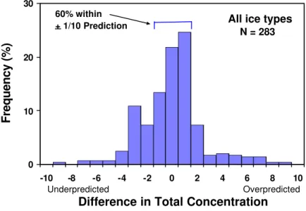
Figure 1 shows a histogram plot of the difference between the predicted and observed ice concentrations for all ice types for the 283 ice regimes. In this case, the actual and predicted concentrations agree for 22% of the cases. In over 60% of the observations, the predicted and observed conditions agree to within ±1/10th concentration. For the rest of the data, there is a slight tendency for the ice charts to underpredict the actual ice concentration. In general, however, there is good agreement between the ice charts and the actual conditions.
0 10 20 30
-10 -8 -6 -4 -2 0 2 4 6 8 10
Difference in Total Concentration
Frequency (%)
N = 283
Underpredicted Overpredicted
All ice types
60% within + 1/10 Prediction
Figure 1: Histogram showing the difference between the predicted and observed concentration for all ice types.
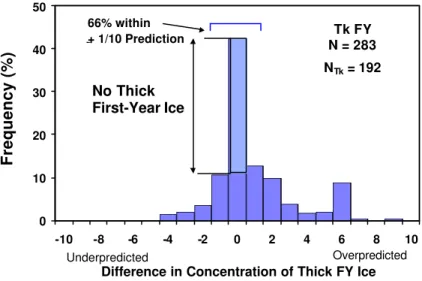
Figure 2 shows a histogram of the difference between the predicted and observed concentrations of thick first- year (FY) ice (i.e. more severe first-year ice conditions). This type of ice was present in 192 of the observations. In approximately 66% of these ice regimes, the CIS ice chart predictions agree to within ±1/10th concentration of the observed concentrations.
Figure 3 shows a histogram of the difference between the predicted and observed concentrations of old, multi- year ice. This type of ice was present in 128 of the observations. In this case, approximately 85% of the observations were within ±1/10th of the predicted concentration. This is extremely good agreement. Note however, that there is a tendency to underpredict the concentration of multi- year ice.
0 10 20 30 40 50 -10 -8 -6 -4 -2 0 2 4 6 8 10
Difference in Concentration of Thick FY Ice
Frequency (%) Underpredicted Overpredicted Tk FY N = 283 66% within + 1/10 Prediction NTk = 192 No Thick First-Year Ice
Figure 2: Histogram showing the difference between the predicted and observed concentration of thick first-year ice.
0 25 50 75
-10 -8 -6 -4 -2 0 2 4 6 8 10
Difference in Concentration of Old Ice
Frequency (%) Underpredicted Overpredicted Old Ice N = 283 total NMY = 128 No MY ice 85% within + 1/10 Prediction
Figure 3: Histogram showing the difference between the predicted and observed concentration of old (multi-year) ice.
ICE VOLUME
As seen in the previous section, there is quite good agreement between the predicted and observed ice concentrations. In this section, a comparison is made of the total “volume” (Vi) of ice. This was determined by summing the product of the ice concentration (Ci) and the ice thickness (hi) for each type of ice. That is
∑
= i i i
i C h
V ( )( ) (1)
where the sum i is carried out for all ice types (including open water, but not multi- year or second- year ice). Since the thickness of second-year and multi- year ice was not known, it could not be taken into account in this analysis. Note, therefore, that this analysis was done for those cases in which there was only first- year ice.
For this analysis, the ice thickness was taken as the maximum ice thickness for each ice type. This is not strictly correct, of course, but it was consistent for both the predicted and observed data. Thus, the values of ice volume calculated represent the maximum volume for both cases. Note that the volume is regarded as a dimensionless quantity since the aerial extent of the ice is not known.
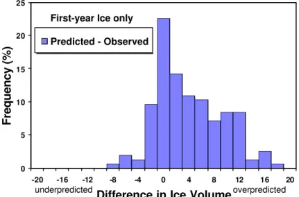
Figure 4 shows the histogram of the difference between the predicted and the observed ice volume. There is a clear indication that, on average, the predicted ice volume is higher than the observed ice volume. Since the data shown in Figure 1 indicated that the ice concentration is usually accurately predicted, the overprediction of ice volume shown in Figure 4 suggests that the ice thickness is often overpredicted on the ice charts.
0 5 10 15 20 25 -20 -16 -12 -8 -4 0 4 8 12 16 20
Difference in Ice Volume
Frequency (%)
Predicted - Observed First-year Ice only
underpredicted overpredicted
Figure 4: Histogram showing the difference between the predicted and observed ice volume. In general, the ice volume was overpredicted.
ICE NUMERALS
The data can be used to predict the Ice Numeral using the Arctic Shipping Pollution Prevention Regulations definition (ASPPR, 1989). The Ice Numeral (IN) is calculated from
∑
= i Ci IMi
IN ( )( ) (2)
where IN is the Ice Numeral, Ci is the Concentration in tenths of ice type “i”, and IMi is the Ice Multiplier for ice type “i”. The term on the right hand side of the equation includes all ice types that are present, including open water. The values of the Ice Multipliers are adjusted to take into account the decay or ridging of the ice by adding or subtracting a correction of 1 to the multiplier, respectively. ASPPR (1989) should be consulted for full details, including the values for the Ice Multipliers for different vessels and ice conditions. The Ice Numeral is unique to the particular ice regime and ship operating within its boundaries.
The comparison of predicted and observed ice conditions was done for 2 different cases: 1. where there was only first- year ice; and
2. with all ice types.
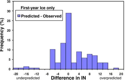
Figure 5 shows a histogram of the difference between the calculated Ice Numerals based on the predicted and observed ice conditions, where there is only first-year ice present (i.e. no second-year or multi- second-year ice present). In general there is good agreement between the predicted and observed Ice Numeral.
0 5 10 15 20 25 30 35 -20 -16 -12 -8 -4 0 4 8 12 16 20 Difference in IN Frequency (%) Predicted - Observed First-year Ice only
underpredicted overpredicted
Figure 5: Histogram showing the difference in the Ice Numeral using predicted and observed ice conditions. This data are based on observations with only first-year ice (i.e. no old ice).
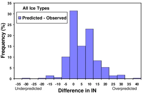
Figure 6 shows a histogram of the difference between the calculated Ice Numerals based on the predicted and observed ice conditions, for all ice conditions. Although there is reasonable agreement on average, the data indicate that the Ice Numeral is often overpredicted using the CIS ice charts. This reflects the data shown in Figure 1 where the CIS ice charts slightly underpredicted the ice concentrations.
0 5 10 15 20 25 30 35 -35 -30 -25 -20 -15 -10 -5 0 5 10 15 20 25 30 35 40 Difference in IN Frequency (%) Predicted - Observed Overpredicted Underpredicted
All Ice Types
Figure 6: Histogram showing the difference in the Ice Numeral using predicted and observed ice conditions for all ice types.
ICE NUMERAL WITHIN AN EGG CODE
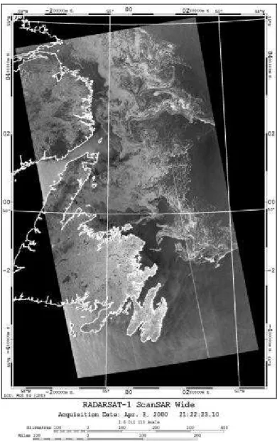
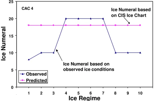
Although ice charts are sub-divided into numerous regions depicting different ice regimes, there is, by necessity, still somewhat coarse resolution. With the current data, it is possible to investigate the local changes in the ice regime within a predicted uniform ice regime on an ice chart. This has been done by calculating the Ice Numerals from the observed ice conditions for a single egg code region of an ice chart. As an illustration of this analysis, Figure 7 shows a single egg code region on an ice chart for NE Newfoundland waters for April 4, 2000. Figure 8 shows the corresponding RADARSAT image for the region. The Ice Numeral is constant with a value of 18 for a CAC4 vessel for the indicated region on the ice chart. However, within this single egg code region, the re were 10 different ice regimes encountered. In this case, the Ice Numeral based on the observed ice conditions varied between 8 and 20. Figure 10 shows a similar analysis for April 6, 2000. In this case, 14 different ice regimes were encountered within a single egg code region of the chart, with corresponding Ice Numerals ranging from –9 to 20.
This analysis was done for 7 different egg-code regions with 2 different vessels. From this limited analysis, there are two things to note:
1. In most cases, the Ice Numeral predicted from ice charts was on average, a reasonable representation of the Ice Numeral calculated using the on board observed ice conditions. In one case, which was not shown here, there was a large difference between the two values.
2. There can be wide variations in the Ice Numeral within a single egg code region, as seen in Figures 9 and 10.
These observations illustrate the importance of continual monitoring of the Ice Numeral, even within an apparent uniform egg code region. Also, it emphasizes one of the fundamental premises of the IRS that the Master makes the decision based on local ice conditions.
Figure 7: CIS Ice Chart for April 4, 2000, for Northeast Newfoundland waters. The ice conditions are detailed using the “Egg Code”.
Figure 8: RADARSAT image for evening April 3, 2001, for Northeast Newfoundland waters.
Copyright CSA 2000
Region of analysis Done in Figure 9
0 5 10 15 20 25 0 1 2 3 4 5 6 7 8 9 10 11 Ice Regime Ice Numeral Observed Predicted CAC 4
Ice Numeral based on observed ice conditions
Ice Numeral based on CIS Ice Chart
Figure 9: Graph showing the variation of the Ice Numeral within a single egg code region from an Ice Chart, Case 1 – April 4, 2000.
-15 -10 -5 0 5 10 15 20 25 0 2 4 6 8 10 12 14 16 Ice Regime Ice Numeral Observed Predicted CAC 4
Ice Numeral based on observed ice conditions
Ice Numeral based on CIS Ice Chart
Figure 10: Graph showing the variation of the Ice Numeral within a single egg code region from an Ice Chart, Case 2 – April 6, 2000.
CONCLUSIONS
The data analyzed here indicated that the CIS ice predictions from ice charts usually present a reliable description of the actual ice conditions. There was no large bias in the predicted ice conditions, although the predictions did show some inaccuracies, as would be expected due to the complexity of ice in nature. This would suggest that the CIS ice charts could be used for strategic route planning.
An analysis of the variability of ice regimes within a single egg code region of an ice chart showed that although the average conditions were usually accurate, there could be considerable variability in the ice conditions within the region. Thus, the ice charts should not be solely used for calculating the Ice Numeral for tactical navigation. Continual on board ice observations are an essential component for correct determination of the Ice Numeral.
ACKNOWLEDGEMENT
The authors would like to acknowledge the support of Victor Santos-Pedro of Transport Canada for funding this study. The work forms part of the background for the scientific basis for the Ice Regime System. The authors would also like to thank Dean Flett of the Canadian Ice Service for supplying the ice chart and the RADARSAT image.
REFERENCES
ASPPR, 1989. Proposals for the Revision of the Arctic Shipping Pollution Prevention Regulations. Transport Canada Report TP 9981, Ottawa. Ont., Canada.
Johnston, M.E. and Gorman, B., 2000, Ice Regimes Encountered during the Transit of the USCGC Healy: 2 April to 25 April 2000. CHC/NRC Report HYD-TR-059, Ottawa, ON, Canada.
Timco, G.W. and Morin, I. 1998. Canadian Ice Regime System Database. Proceedings 8th International Offshore and Polar Engineering Conference ISOPE’98, Vol II, pp 586- 591, Montreal, P.Q., Canada.
Timco, G.W., Frederking, R.M.W. and Santos-Pedro, V.M. 1997. A Methodology for Developing a Scientific Basis for the Ice Regime System. Proceedings 7th Offshore and Polar Engineering Conference ISOPE97, Vol. II, pp 498-503, Honolulu, Hawaii, USA.