Science Arts & Métiers (SAM)
is an open access repository that collects the work of Arts et Métiers Institute of
Technology researchers and makes it freely available over the web where possible.
This is an author-deposited version published in:
https://sam.ensam.eu
Handle ID: .
http://hdl.handle.net/10985/18388
To cite this version :
Adrien SCHEUER, Guillaume GRÉGOIRE, Emmanuelle ABISSET-CHAVANNE, Francisco
CHINESTA, Roland KEUNINGS - Modelling the effect of particle inertia on the orientation
kinematics of fibres and spheroids immersed in a simple shear flow - Computers and Mathematics
with Applications - Vol. 79, n°3, p.539-554 - 2020
Any correspondence concerning this service should be sent to the repository
Administrator :
archiveouverte@ensam.eu
Modelling the effect of particle inertia on the orientation
kinematics of fibres and spheroids immersed in a simple
shear flow
A. Scheuer
a,b,∗, G. Grégoire
c, E. Abisset-Chavanne
a, F. Chinesta
d, R. Keunings
b aICI - High Performance Computing Institute & ESI Group Chair, Ecole Centrale de Nantes, Rue de la Noe 1, F-44300 Nantes, France bICTEAM, Université catholique de Louvain, Bat. Euler, Av. Georges Lemaitre 4, B-1348 Louvain-la-Neuve, BelgiumcLaboratoire Matière et Systèmes Complexes (MSC), University Paris-Diderot, CNRS UMR 7057, F-75205 Paris, CEDEX 13, France dPIMM & ESI Group Chair, ENSAM ParisTech, Boulevard de l’Hôpital 151, F-75013 Paris, France
Keywords: Particle inertia Jeffery’s equation Fibre suspension Spheroid a b s t r a c t
Simulations of flows containing non-spherical particles (fibres or ellipsoids) rely on the knowledge of the equation governing the particle motion in the flow. Most models used nowadays are based on the pioneering work of Jeffery (1922), who obtained an equation for the motion of an ellipsoidal particle immersed in a Newtonian fluid, despite the fact that this model relies on strong assumptions: negligible inertia, unconfined flow, dilute regime, flow unperturbed by the presence of the suspended particle, etc. In this work, we propose a dumbbell-based model aimed to describe the motion of an inertial fibre or ellipsoid suspended in a Newtonian fluid. We then use this model to study the orientation kinematics of such particle in a linear shear flow and compare it to the inertialess case. In the case of fibres, we observe the appearance of periodic orbits (whereas inertialess fibres just align in the flow field). For spheroids, our model predicts an orbit drift towards the flow-gradient plane, either gradually (slight inertia) or by first rotating around a moving oblique axis (heavy particles). Multi-Particle Collision Dynamics (MPCD) simulations were carried out to assess the model predictions in the case of inertial fibres and revealed similar behaviours.
1. Introduction
Suspensions of rigid non-spherical particles (ellipsoids or fibres) are encountered in many biological and engineering systems, including aerosols, papermaking or short-fibre composite moulding processes such as SMC. Modelling the evolution of the flowing microstructure is thus necessary to predict the impact of the particles on the rheology of the suspension, as well as the motion and orientation kinematics of the suspended particles. In the context of composite manufacturing, changes in fibre orientation correspond to changes in the final mechanical properties of the part, and similarly in the paper and pulp industry, the orientation distribution of cellulose fibres in the final product is a key factor of its quality.
Such suspensions have been extensively studied at different modelling scales. Depending on the level of details and accuracy required for a particular application, one may want to address a problem at a specific scale or even to adopt a
∗ Corresponding author at: ICTEAM, Université catholique de Louvain, Bat. Euler, Av. Georges Lemaitre 4, B-1348 Louvain-la-Neuve, Belgium.
E-mail addresses:Adrien.Scheuer@ec-nantes.fr,Adrien.Scheuer@uclouvain.be(A. Scheuer),Guillaume.Gregoire@univ-paris-diderot.fr(G. Grégoire),
Emmanuelle.Abisset-Chavanne@ec-nantes.fr(E. Abisset-Chavanne),Francisco.Chinesta@ensam.eu(F. Chinesta),Roland.Keunings@uclouvain.be
Fig. 1. General modelling framework composed of nine conceptual bricks exploring the three scales involved in the multi-scale description of a suspension
of particles [14]. For each scale, the main challenge (either conceptual or computational) is also mentioned.
multi-scale approach by ‘‘upscaling’’ the properties across the scales. We propose hereunder a succinct overview of the three different modelling scales usually considered in the context of fibre suspensions and refer to the review by Petrie [1] or the recent monograph [2] for further details.
•
Microscopic scale: the scale of the particle itself. Each particle’s orientation is described by a unit vector along its symmetry axis and Jeffery’s theory [3] (see below) lays the foundation for most models governing its kinematics.•
Mesoscopic scale: the scale of a population of particles, whose orientation state is described by a probability densityfunction (pdf). Such pdf lies both in physical (space and time) and conformational space and provides a complete, unambiguous description of the fraction of particles oriented along a given direction at any location and any time. Its evolution is given by a Fokker–Planck equation, whose solution is often impracticable due to the inherent high-dimensionality of the problem (the so-called ‘‘curse of high-dimensionality’’).
•
Macroscopic scale: the scale of the part, whose conformation state is often characterized by the first moments of the aforementioned probability density function. For fibres, the second-order orientation tensor [4] is often chosen as a coarse, yet concise, description of the orientation state in the part, and its time evolution is governed by the Folgar– Tucker model [4,5] built directly upon Jeffery’s theory. Macroscopic models are often easy-to-compute and offer a crude description of the orientation state. They usually rely however on mathematical closure approximations [6–9] whose impact is quite unpredictable.Over the last few years, we proposed a modelling framework to describe suspensions of fibres and ellipsoids immersed in a Newtonian matrix based on the dumbbell model (originally initiated in [10]) and we extended this model to successively address more complex situations [2]. We showed a new way to obtain Jeffery’s kinematics for a fibre by considering a Stokesian hydrodynamic drag force acting on the dumbbell beads [11]. We were then able to activate bending mechanisms by considering higher gradients of the fluid velocity field at the scale of the particle [12]. Suspensions of charged fibres (as carbon nanotubes for example) were then described using the same modelling framework in [13]. In [14], we proposed a systematic multi-scale approach composed of nine conceptual bricks aimed at describing a suspension of particles using the dumbbell model. At each modelling scale are raised the questions of describing the conformation of the suspended particles, the evolution of this conformation, and the contribution to the stress (rheology) of the particles. This systematic approach is summarized inFig. 1and we refer the interested reader to [14] for further details and the application of this approach to a dilute suspension of rigid fibres in a Newtonian fluid. This modelling framework was also applied successfully to describe rigid clusters composed of rods [14]. Recently, we adapted the dumbbell model to propose a description of fibre suspensions subject to wall and confinement effects (when the flow gap is narrower than the fibre length) [15,16]. In the present work, the dumbbell model is enriched to study the impact of particle inertia on the kinematics of a suspended fibre or spheroid (axisymmetric ellipsoid).
Studies dedicated to the effects of inertia on the dynamics of non-spherical particles in a flow usually make a distinction between fluid inertia and particle inertia. The former is often characterized by the Reynolds number, defined as Re
=
ρfγ˙L2µ (with
ρ
f the fluid density,γ
˙
the shear rate, L the particle length andµ
the fluid viscosity), and the latter measured by theStokes number St
=
ρpρfRe
=
ρpγ˙L2
µ (with
ρ
pthe density of the inertial particle) [17]. Hence, four distinct scenarios can beconsidered.
In his pioneering work, Jeffery [3] derives the orientation kinematics of an inertialess, force-free, torque-free spheroid immersed in a Stokes (Reynolds number zero) linear shear flow of Newtonian fluid. His model predicts that such a spheroid is constrained in one of an infinite set of (one-parameter) closed orbits, the so-called ‘‘Jeffery orbits’’. The particular choice of orbits, bounded on the one hand by a circular motion in the shear plane (tumbling) and on the other hand by a rolling motion around the vorticity axis (log-rolling), depends on the initial orientation. The resulting motion is often referred to as
kayaking.
There is a long history of deriving equations of motion for suspended particles taking into account effects of fluid inertia. Saffman [18] addressed the impact of fluid inertia dynamics of a nearly spherical particle in a shear flow, and Hinch and Leal [19] discussed later the important role of fluid inertia on the kinematics of inertialess particles. More recently, Ding and Aidun [20] solved the Boltzmann equation to study the impact of strong fluid inertia on the motion of solid particles (cylinders and ellipsoids) and then Subramanian and Koch examined the inertial effects of fibres [21] and ellipsoids [22] motion in a shear flow using a generalization of the reciprocal theorem for Stokes flow. Yu et al. [23] studied numerically the rotation behaviour of both prolate and oblate spheroids in Couette flow at moderate Reynolds numbers using the distributed Lagrangian multiplier based fictitious domain. Over the last few years, there has been a surge of interest, lead by Lundell and co-authors, in determining the effects of fluid and particle inertia, either by analytical analysis and perturbation methods [24–26] or lattice Boltzmann simulations [27–31], depicting a rich dynamics containing several bifurcations between rotational states due to inertial effects.
The effect of particle inertia alone was investigated by Altenbach [32,33] for a fibre suspended in several homogeneous creeping flows. They observed a particle drift towards the flow plane for flow fields with dominant vorticity (elliptic and rotational flows). Lundell and Carlsson [17] found a similar behaviour for inertial ellipsoid in a linear shear flow: for small St the particle slowly drifts from its kayaking motion towards the flow plane, whereas for larger values of St, rotation around an oblique axis is exhibited [17,34].
In this paper, we propose a model describing the orientation kinematics of inertial particles based on a dumbbell representation of the suspended fibre. This microstructural approach is then generalized to suspended ellipsoids in a straightforward way, and we are able to provide an equation of motion, which is the counterpart of the classical Jeffery equation for inertial particles. From this microscopic kinematics, we then pave the way towards a micro–macro description of suspensions of such particles.
The remainder of the paper is organized as follows. The modelling framework and the dynamical system describing the orientation behaviour of suspended inertial particles are presented in Section2. Sections3and4show some numerical simulations illustrating the kinematics of particles, fibres and spheroids, immersed in a simple shear flow, either by integrating the dynamical system at the microscopic scale (scale of a single particle) or by solving directly the Fokker–Planck equation describing the evolution of the orientation probability density function of a population of suspended particles. In Section5, we present qualitative comparisons of predictions using our model and direct numerical simulations performed using Multi-Particle Collision Dynamics (MPCD). Finally, Section6draws the main conclusions of our work and discusses some observations as well as possible extensions to our model addressing the impact of inertia on the orientation of particles immersed in a fluid flow.
Remark 1. In this paper, we consider the following tensor products, assuming Einstein’s summation convention:
•
if a and b are first-order tensors, then the single contraction ‘‘·
’’ reads (a·
b)=
ajbj;•
if a and b are first-order tensors, then the dyadic product ‘‘⊗
’’ reads (a⊗
b)jk=
ajbk;•
if a and b are respectively second and first-order tensors, then the single contraction ‘‘·
’’ reads (a·
b)j=
ajkbk;•
if a and b are second-order tensors, then the double contraction ‘‘:
’’ reads (a:
b)=
ajkbkj.2. Kinematics of inertial fibres and spheroids
In this section, we first derive the equations ruling the dynamical system describing a suspended fibre immersed in a Newtonian fluid of viscosity
η
and then extend our microscopic model for a suspended spheroid. The end of this section is an attempt towards a multi-scale description of a population of suspended inertial particles: first at the mesoscopic scale, considering the pdf of orientation and its associated Fokker–Planck evolution, and then at the macroscopic scale, retaining only the first moments of the pdf.2.1. Microscopic modelling
2.1.1. Dumbbell model of an inertial fibre
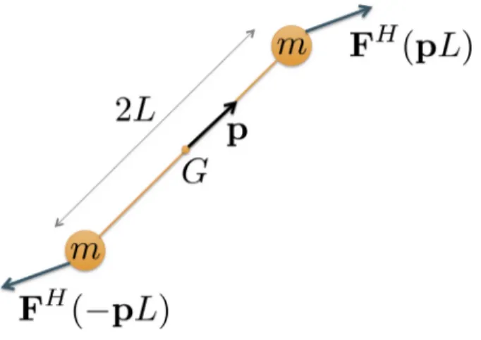
A fibre is modelled as a rigid dumbbell consisting of a rod linking two beads on which act hydrodynamic forces, as depicted inFig. 2. In this work, the mass of the fibre is not neglected and we thus consider that each bead has a mass m. The rod’s length is 2L and its 3D-orientation is given by the unit vector p located at the rod centre of gravity G and aligned with its axis.
Fig. 2. Dumbbell representation of a fibre.
The hydrodynamic force FHacting on each bead depends on the difference of velocities between the fluid at the bead
location and the bead itself. For the bead located at pL, the former is given by v0
+ ∇v
·
pL (with v0the velocity of the fluidat the centre of gravity G) and the latter byx
˙
G+ ˙
pL (withx˙
Gthe velocity of the centre of gravity G). The hydrodynamic forceacting on the bead located at pL thus reads
FH(pL)
=
ξ
(v0+ ∇v
·
pL−
(x˙
G+ ˙
pL)),
(1)where
ξ
is a friction coefficient.Imposing Newton’s second law of motion and rotation on the whole dumbbell would provide relations governing the behaviour of the dynamical system. We chose equivalently to apply d’Alembert’s principle and introduce the so-called inertial
forces as forces acting on the dumbbell’s beads. Imposing Newton’s second laws then reduces to enforcing balance of forces
and torques.
The inertial pseudo-forces FIacting on each bead simply scale with the acceleration of the bead and thus read (for the bead located at pL)
FI(pL)
= −
m(x¨
G
+ ¨
pL),
(2)with m the mass of the bead. Balance of forces yields
∑
F
=
0⇐⇒
FH(pL)+
FI(pL)+
FH(−pL)
+
FI(−pL)
=
0 (3)⇐⇒
2ξ
(v0− ˙
xG)−
2mx¨
G=
0 (4)or
mx
¨
G=
ξ
(v0− ˙
xG).
(5)Due to the symmetry of the problem, the only possibility for the resulting torque to vanish is that the total force applied on each bead acts along p, that is
∑ τ =
0⇐⇒
FH(pL)+
FI(pL)=
α
p,
(6)with
α ∈
R. Thus, using Eq.(5), we can writeξ
L(∇v
·
p− ˙
p)−
mLp¨
=
α
p.
(7)Taking into account that p
·
p=
1, and thusp˙
·
p=
0 andp¨
·
p+ ˙
p· ˙
p=
0, we can obtain the value ofα
by premultiplying Eq.(7)by pα = ξ
L(∇v
:
(p⊗
p))+
mL(p˙
· ˙
p),
(8)Inserting the expression of
α
back in(7)givesξ
(∇v
·
pL− ˙
pL)−
mpL¨
=
ξ
L(∇v
:
(p⊗
p))p+
mL(p˙
· ˙
p)p,
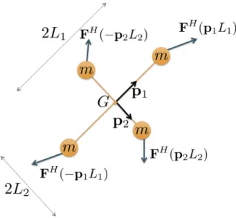
(9) orFig. 3. Bi-dumbbell representation of a 2D spheroid.
To summarize, the second-order dynamical system governing the kinematics of an inertial suspended fibre is
mx
¨
G=
ξ
(v0− ˙
xG) (11)mp
¨
=
ξ
(∇v
·
p−
(∇v
:
(p⊗
p))p− ˙
p)−
m(p˙
· ˙
p)p.
(12)The first equation describes the translational displacement of the fibre, whereas the second equation governs its rotational motion. Note that Eq.(12)contains the expression of the classical inertialess Jeffery’s equation
˙
p
= ∇v
·
p−
(∇v
:
(p⊗
p))p,
(13)for infinite aspect ratio ellipsoids (rods). Thus, we observe that when the mass of the dumbbell beads is set to zero, we recover the usual kinematics: the rod centre of gravity is moving with the fluid velocity, v0
= ˙
xG, and the orientation kinematics aregiven by Jeffery’s equation (13).
The orientation kinematics equation (12)is the same that the ones derived independently by Altenbach and co-authors [32,33] using a different approach based on the expression of the hydrodynamic moment exerted on the fibre provided by Brenner [35]. We thus showed here an alternative way of recovering this model using a dumbbell description, which in our case can be generalized directly to suspended ellipsoids.
2.1.2. Dumbbell model of an inertial spheroid
Extending this modelling approach to inertial ellipsoids is now straightforward. As depicted inFig. 3, an ellipsoid is described as a bi-dumbbell in 2D (tri-dumbbell in 3D) with again hydrodynamic forces acting on the inertial beads. In the remainder of this paper, we restrict our discussions to spheroids, that is axisymmetric ellipsoids. In the case of inertialess fibres, such a description proved to recover successfully Jeffery’s kinematics for spheroids [14]
˙
p
=
Ω ·
p+
λ
(D·
p−
(D:
(p⊗
p))p),
(14)where D and
Ω
are respectively the symmetric and skew-symmetric parts of the velocity gradient∇v and
λ
is the axisymmetric ellipsoid shape factor (defined from the ellipsoid aspect ratio r)λ =
r2−
1 r2+
1=
L2 1−
L22 L2 1+
L22.
(15)Using the same rationale as in the case of rods: introducing inertial forces (d’Alembert principle) and enforcing balance of forces and torques, we obtain the dynamical system governing the behaviour of a suspended inertial spheroid immersed in a Newtonian fluid. The system is actually the same as the one obtained for fibres, except that it now contains the general form of Jeffery’s equation (Eq.(14))
mx
¨
G=
ξ
(v0− ˙
xG) (16)The system(16)–(17)is the most general since Eqs.(11)–(12)are recovered when
λ =
1 (rods can be seen as infinite aspect ratio ellipsoids); therefore we will use this formulation for the rest of this paper.Besides, this system can be rewritten as a system of first-order differential equations
˙
xG=
vG (18)˙
vG=
ξ
m(v0−
vG) (19)˙
p=
w (20)˙
w=
ξ
m(Ω ·
p+
λ
(D·
p−
(D:
(p⊗
p))p)−
w)−
(w·
w)p.
(21) 2.1.3. Dimensional analysisFor the sake of completeness, we briefly show in this section how to obtain a dimensionless formulation of the orientation kinematics(17). Introducing the dimensionless time
˜
t=
ξmt, the first and second derivatives with respect to time now read d· dt
=
ξ m d· d˜t and d2· dt2=
ξ 2 m2 d2·d˜t2. The dimensionless dynamical system is thus given by
d2p d
˜
t2=
mξ
(Ω ·
p+
λ
(D·
p−
(D:
(p⊗
p))p))−
dp dt˜
−
(
dp d˜
t·
dp d˜
t)
p.
(22)If we normalize the fluid velocity gradient by the magnitude of the strain rate tensor
γ =
˙
√
2D:
D,Ω = ˙
γ ˜Ω
and D= ˙
γ ˜
D, we can now writed2p d
˜
t2=
St (˜
Ω ·
p+
λ
(D˜
·
p−
(D˜
:
(p⊗
p))p))−
dp d˜
t−
(
dp dt˜
·
dp dt˜
)
p,
(23)where the Stokes number St
=
mξγ˙ is a dimensionless number characterizing the intensity of particle inertia.2.2. Mesoscopic description of a population of inertial particles
We now move to a population of suspended particles. Instead of describing each particle conformation individually, the microstructure conformation may be characterized by a probability density function – pdf–
ψ
. Since this paper mainly focuses on the orientation dynamics, we will assume thatψ = ψ
(t,
p, ˙
p), that is we consider the orientation distribution independent of the space coordinates. Contrary to the inertialess case where particles are assumed to move with the fluid velocity, here particles should be transported using the equation of motion(16). Moreover, it is important to notice that when inertia is considered, the particle rotational velocityp is also a conformation coordinate of the pdf. Hence, balance of˙
probability yields the following Fokker–Planck equation∂ψ
∂
t+ ∇
p·
(p˙
ψ
)+ ∇
p˙·
(p¨
ψ
)=
0,
(24)where the angular dynamics of the particle given by Eq.(17)is used forp, and
¨
∇
pand∇
p˙are the gradients in conformation space. The pdfψ
is subject to the normalization condition∫ ∫
ψ
(t,
p, ˙
p) dp dp˙
=
1.
(25)Moving from a single particle to a mesoscopic description of a population of particles by a pdf is a straightforward step. However, the difficulty in practice is the intrinsic high-dimensionality of the Fokker–Planck equation whose solution is often intractable using standard methods. Indeed, in the general case above (Eq.(24)), the pdf actually lies in a 5-dimensional space: 1 for t, 2 for p (a unit vector in 3D can be represented by two angles) and 2 forp. In Section
˙
4, we present some results obtained by solving a reduced version of this Fokker–Planck equation in the case of a 2D flow. Addressing 3D flows and the impact of inertia on the translational motion of the particles through the complete Fokker–Planck equation (see below) may be possible using a separation technique such as the PGD [36–38] to circumvent the so-called ‘‘curse of dimensionality’’. Over the last decade, the PGD method was successfully applied to Fokker–Planck equations of high dimensions (up to 20) encountered in kinetic theory problems [39].Addressing the translational and rotational movement of the population of particles at once using a Fokker–Planck approach is an alternative route that is out of the scope of this paper. In that case, we may consider the pdf
φ
(x, ˙
x,
t,
p, ˙
p) along with its associated Fokker–Planck evolution equation∂φ
∂
t+ ∇
x·
(x˙
φ
)+ ∇
x˙·
(x¨
φ
)+ ∇
p·
(p˙
φ
)+ ∇
p˙·
(p¨
φ
)=
0,
(26)where Eqs.(16)and(17)are used forx and
¨
p respectively. However, the dimensionality of that equation now jumps to 11¨
(3 for x, 3 forx, 1 for t, 2 for p and 2 for˙
p).˙
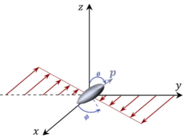
Fig. 4. Spheroid particle placed in a linear shear flow. The flow is in the x-direction, the gradient in the y-direction and the vorticity in the z-direction. The
orientation of the principal axis of the particle is given by the unit vector p.
2.3. Towards a macroscopic model
Deriving a macroscopic model for the orientation of inertial particles appears to be a tedious task, especially since new macroscopic tensors need to be defined, along with corresponding closure approximations. InAppendix A, we pave the way towards such a macroscopic model and underline the difficulties arising when trying to obtain a closed model.
3. Numerical simulation of a single particle in a simple shear flow We consider a simple shear flow given by v
=
[ ˙
γ
y 0 0]
T. This flow is depicted inFig. 4. The flow is in the
x-direction, the gradient in the y-direction and the vorticity in the z-direction. The orientation of the particle is described by
the unit vector p aligned with its principal axis, that is, using a spherical coordinate system, by the two angles
φ
andθ
. We solved numerically the dynamical system describing the motion of a suspended particle and discuss in this section the various behaviours observed when starting from different configurations. In practice, we solved Eqs.(18)–(21)using an implicit Adams–Moulton scheme of order 2 (trapezoidal rule) and a Newton–Raphson method to solve the nonlinear problem at each time step. In the particular case where m=
0, Eqs.(18)–(21)are singular and we simply solve the classical (inertialess) Jeffery model.For the sake of clarity, we first show some results when the particle principal axis is initially aligned in the flow-gradient plane (
θ
0=
π2) and then explore the general case. The reason is that in the general case the orbits are no longer periodic andwe observe a drift of the particle trajectories towards the flow-gradient plane, as discussed below.
3.1. Particle initially aligned in the flow-gradient plane
We first study the orientation kinematics of rigid fibres.Fig. 5depicts the components px
=
[p]xand py=
[p]yof theunit vector pointing in the direction of the fibre, as well as the angle
φ
giving its orientation in the xy-plane. The fibre is initially at rest and lies in the flow-gradient plane with (φ
0, θ
0)=
(
9π10
,
π
2
)
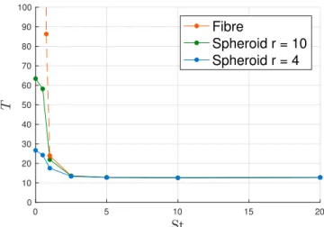
. The results are shown for various values of the Stokes number from 0 (inertialess case) to 5. Without particle inertia (grey curve), the particle simply aligns in the flow direction (equilibrium position). Once particle inertia is introduced, we now observe periodic orbits, since inertia induces a jump of the fibre over the equilibrium position. For slightly inertial fibre, the period can be very long (the inertialess case may be seen as the limit case with an infinite period).Fig. 7shows the evolution of the orientation period as a function of the Stokes number. We can also notice that the minimum orientation speed is reached after the particle has jumped over the equilibrium position. Another consequence of particle inertia on the orientation kinematics is the delay observed when starting the motion from rest.
Similarly,Fig. 6depicts the situation for an inertial spheroid of aspect ratio r
=
4 under the same conditions. According to Jeffery model, inertialess ellipsoids already exhibit periodic tumbling orbits, where the particle aligns most of the time with the flow lines and rotates quickly half a turn periodically (Fig. 6, grey curve). With particle inertia, the same kinematics is observed but the period is now shortened. The symmetry of the orbit shape around the equilibrium position is also lost when particle inertia is considered: the particles approach the aligned orientation quite quickly and depart from it slowly. Again, a delay at the start of the shear flow is evidenced and of course, the more massive the spheroid is, the longer is the delay.Fig. 7shows the evolution of the orientation period as a function of the Stokes number in the case of fibres (which can be seen as spheroids of infinite aspect ratio) (orange line), spheroids of aspect ratio r
=
10 (green) and spheroids of aspect ratior
=
4 (blue). Massive particles tend to rotate with constant angular velocity once put in motion, as shown inFigs. 5and6. In the case of a shear flow with shear rateγ =
˙
1, this angular velocity isφ = −
˙
0.
5 (the particle rotates with the vorticity), hence an angular period T=
4π
, as reported inFig. 7.Fig. 5. Evolution of the orientation of a fibre immersed in a shear flow for various values of the Stokes number.
Fig. 6. Evolution of the orientation of a spheroid of aspect ratio r=4 immersed in a simple shear flow for various values of the Stokes number.
3.2. Particle initially not aligned in the flow-gradient plane
We now move to the general case and focus on the kinematics of spheroids.
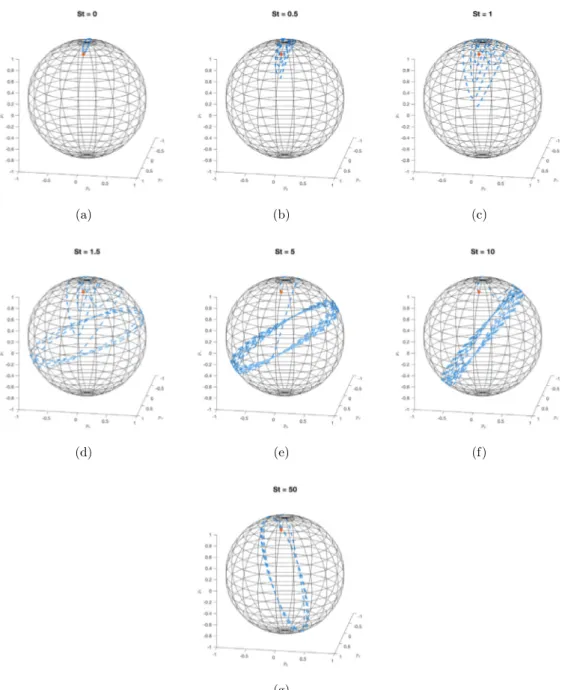
InFig. 8, we depict the orientation trajectories for spheroids of aspect ratio r
=
10 for different values of the Stokes number. The initial configuration of the particles is(φ
0, θ
0) = (
0,
π8)
and is shown in orange. In each case, the simulation was run for t
γ ∈ [
˙
0,
250]
. The orientation is shown as a point on the unit sphere, which is the direction of the unit vector oriented along the particle principal axis.A inertialess spheroid (Fig. 8(a)) exhibits the classical kayaking motion, with the so-called periodic Jeffery orbits. When inertial effects are introduced, the trajectories do not follow describe periodic orbits anymore. At low Stokes number, the particle is seen to spiral outwards, that is we observe a slight drift of the particle trajectory towards the flow-gradient plane (Figs. 8(b)–8(c)). When the particle inertia is further increased a dramatic change in the orientation kinematics occurs. The
Fig. 7. Rotation period of a fibre (orange line), a spheroid of aspect ratio r=10 (green) and a spheroid of aspect ratio r=4 (blue) as a function of the Stokes number. (For interpretation of the references to colour in this figure legend, the reader is referred to the web version of this article.)
spheroid now spirals a little bit before rotating around a tilted axis, that will gradually align with the z-axis with increasing timeFigs. 8(d)–8(g). As shown inFig. 8, the angle of this tilted axis with the flow gradient plane depends on the intensity of inertial effects, but also on the initial orientation and aspect ratio of the spheroid.
This complex and somehow strange behaviour was also observed by Lundell and Carlsson [17], who studied the impact of particle inertia using a different but related approach. They obtained an equation of motion for the particle by coupling the analytical expression of the hydrodynamic torque on the spheroid (given by Jeffery) with the angular-momentum equation for the particle. In particular, the rotation of the spheroid around a tilted axis is clearly shown in Fig. 4 of [17].
4. Numerical simulation of a population of particles in a simple shear flow
In this section, we show the feasibility of solving the Fokker–Planck equation describing the orientation kinematics of a population of inertial particles. For the sake of simplicity, we consider a homogeneous population of 2D spheroids immersed in a shear flow. In this case, the orientation of a single particle in the xy-plane is described by the angle
φ
and the pdf readsψ = ψ
(φ, ˙φ
). Eq.(24)thus reduces to∂ψ
∂
t+ ∇
φ·
(˙
φψ
)+ ∇
φ˙·
(φψ
¨
)=
0,
(27)where
φ = −
¨
sin(φ
) [p]¨
x+
cos(φ
) [p]¨
yandp is given by Eq.¨
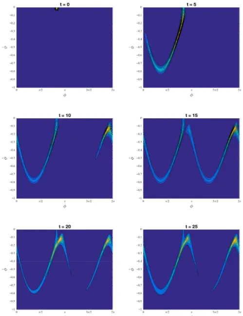
(17).Fig. 9depicts snapshots of the probability density function
ψ
(φ, ˙φ
) obtained by solving the Fokker–Planck equation(27)for a population of 2D ellipsoids with St
=
1 and aspect ratio r=
4 initially at rest around the orientationφ
0=
56π.We used a finite-difference solver and a 4th-order Runge–Kutta scheme for the time integration. The problem being purely convective, a slight artificial diffusion is used to stabilize the numerical solution. The grid size is here (nφ
,
nφ˙)=
(241,
81) and∆t=
5·
10−3s. We observe that the population of particles rotates in the shear flow, and slows down when approachingthe orientations
φ =
kπ
, k∈
Z, that is the orientation where the principal axis of the particle is oriented in the flow field. Due to the inertial effects, the points where the magnitude of the orientation speed is the smallest are not exactly atφ =
kπ
. 5. Comparisons with multi-particle collision dynamics simulationsWe propose here to compare the predictions given by our dumbbell model with direct numerical simulations using Multi-Particle Collision Dynamics (MPCD) in the case of inertial fibres.
The MPCD algorithm [40] has been developed to take into account the solvent–solute interactions, even if those effects are due to thermal fluctuations. The main idea consists in using particles and in mimicking the mesoscopic behaviours as it has been done in other techniques such as Dissipative Particles Dynamics [41,42] or Smooth Particles Hydrodynamics [43]. As in toy models, where the detail of the microscopic physics is dismissed to retain only the pertinent symmetries, MPCD schemes are based on peculiar symmetries: the trajectories of the particles are stochastic but verify classical laws of conservation. Here we propose to set our system in a micro-canonical ensemble. So we impose the conservation of the number of particles, the volume and the energy. The linear momentum and the angular momentum are also conserved. To insure the extensive property of the system, these constraints have to be checked at the scales of the coarse-graining.
The usual MPCD algorithm [44] consists of two steps. First particles move through a streaming process during a time step∆t (Eq.(28)). The ballistic motion of the particles insures the advection of the fluid. This process is off-lattice. Secondly,
Fig. 8. Orientation trajectories of spheroids of aspect ratio r =10 with initial condition(φ0, θ0) = (0,π8
)
(in orange) for different values of the Stokes number. (For interpretation of the references to colour in this figure legend, the reader is referred to the web version of this article.)
particles collide (Eqs.(29)and(30)). In each cell
ξ
of an regular grid of mesh size d0, the particles get the momentum ofthe centre of mass except some fluctuations. These ones are updated with a random rotationΩξt(Eq.(30)). Because of the linearity of the rotation and because it conserves the scalar product, this so-called collision conserves the linear momentum and the kinetic energy:
rti+∆t
=
rti+
∆t vti,
(28) Vt ξ=
1∑
mi∑
i∈ξ mivti,
(29) vti+∆t=
Vtξ+
Ωξt[
vti−
Vtξ]
.
(30)But, it has been shown that there is a lack of conservation of the Galilean boost [45] and that the conservation of the angular momentum is violated [46] in this algorithm.
Fig. 9. Snapshots of the pdfψobtained by solving the Fokker–Planck equation(27)for a population of 2D ellipsoids with St=1 and aspect ratio r=4 initially at rest about the orientationφ0=56π.
The first problem is due to the presence of a fixed grid. This is solved by using a global stochastic displacement
δ
tof thegrid [45]. The second problem has been cured by many variations [44,47,48]. But usually angular momentum and kinetic energy cannot be both conserved in micro-canonical ensemble. We propose an adapted algorithm where positions and velocities follow the same stochastic rotation around the position Rt
ξ of the centre of mass: Rtξ
=
∑
1 mi∑
i∈ξ mirti,
(31) Vtξ=
∑
1 mi∑
i∈ξ mivti,
(32) vti+∆t=
Vt ξ+
Ωξt[
vti−
Vtξ]
,
(33) rti=
Rtξ+
Ωξt[
rti−
Rtξ]
,
(34) rt+∆t i=
r t i+
∆t v t+∆t i+
δ
t.
(35)Table 1
Table of MPCD parameters.
nr ω nδ min(δ) ρ ℓ mf ∆t d0 mT kBT N re
1986 π/2 54 0.01 4 128 1 1 1 100 1 200 0.5
In this scheme, we neglect the time of collision and the energy cost of the rearrangements occurring during it (Eqs.(33)
and(34)). Therefore, both the angular momentum and the kinetic energy are constant during collisions. Eq.(35)contains the streaming step and the jiggling of the grid.
To decrease the computing time, we adapt the initial two-dimensional algorithm of [40] to the three-dimensional problem. The operatorsΩξt are chosen in a set of nr given rotations of a single angle
ω
around nr axes which are regularlydistributed over the unitary sphere. For any axis of vector u, we added the constraint to use the opposite axis, i.e.
−u. Then
there is no net rotation in average.Equivalently, nδthree-dimensional displacements
δ
of the grid are stochastically drawn from an urn without replacement, but periodically refilled such that the mean< δ >
nδ=
0. The maximum displacement along each direction is also less thand0
/
2.We will show elsewhere [49] that the obtained fluid is a Maxwell gas for which the linear hydrodynamic laws hold. And we are able to measure classical transport coefficients as a function of nr, nδ, the angle
ω
and the density of the fluidρ
.We modelled a rodRas a line of N equally disposed beads, with no width, but with a mass mb. The order of magnitude
of the inter-distance reis d0, so each microscopic part of the rod follows the microscopic motion of the fluid but we study a
macroscopic rod, i.e. N
≫
1. The mass of the bead mbis a free parameter and can be different from the mass of fluid particles mf. The dynamics of beads is composed of two steps. First they exchange momentum and energy with the ambient fluid.Therefore, they take part in the sum of Eqs.(31)–(33). This implies also that the rod is thermalized at the fluid temperature. Secondly, the assembly of beads follows the kinematics of a perfect solid. So the fibre gets a motion of translation at a velocity vt G, vtG
=
1 N∑
i∈R vti,
and a rotation around the axis of the angular momentum in the framework of the centre of mass of the rod rtG, Lt
G
=
∑
i∈R
mi(rti
−
rtG)×
vti,
with a rotation speed
α
t= |L
tG
|
/
J, where J is the momentum of inertia. We consider that nothing happens at a smaller timescale than∆t. So we compute the kinematics at the first order, using an explicit Euler algorithm. The updated velocity of
each bead is just its relative displacement during this step.
We first wanted to use a cubic system of linear size
ℓ
with periodic boundary conditions for the positions and the Lees– Edwards conditions for the velocity. Such boundary conditions conserve the temperature of the MPCD fluid alone. But the kinematics of the rod are purely deterministic. This leads to a total decrease of energy and creates a heat well. To maintain a constant energy we choose to introduce a third sort of particles constituting a thermostat. To do so, these particles of mass mTenter in the collision process of MPCD when we compute the properties of centre of mass (Eqs.(31)and(32)). The streaming process does not hold for the thermostat particles. We fix their positions at constant values in the physical framework, and so they follow the stochastic motion
δ
on the grid. Initially, there is a layer of particles at y∈ [−
d0/
2;
0[
and another one at y∈ [
ℓ; ℓ +
d0/
2[
. Their velocity is updated to mimic a moving surface at temperature T :vi
= [ ˙
γ ℓ
Θ(y−
ℓ
)+
η
0 0]
T,
whereΘis the Heaviside function and
η
is a Gaussian distributed noise with a variance kBT/
mT. We will show elsewhere [49]that this thermostat succeeds in maintaining the temperature constant. However there is a discrepancy between the temperature we want to reach Tr and the measured temperature Tm. This discrepancy can be overcome since there is a
linear dependency between Trand Tmfor a given system.
In MPCD algorithms, the fluid is a gas. To avoid longitudinal waves, one has to check that the Mach number remains negligible : Ma
≪
1. This implies a condition on the shear rate :γ ℓ ≪ √
˙
kBT/
mf. Here, we setγ =
˙
1/
320. The value of theother MPCD parameters is listed inTable 1.
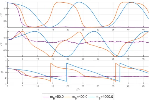
With these three types of particles, we get a thermostated sheared fluid with an infinitely thin but inertial rod. We follow the rod dynamics for different bead mass mb. Our direct simulations presented inFig. 10are consistent with the results of
our dumbbell model (Fig. 5), except that MPCD algorithm is intrinsically driven by the thermal fluctuations. Thus, when mb
is low, the rod performs one flip in the flow and then stops its rotation. Although the mechanical model does not allow any rotation, the MPCD dynamics shows a regime of stochastic motion (see the purple curve inFig. 10). The amplitude of this motion depends on the length of the rod. As there are more beads, the stochastic rotation is smoothened. For larger mass, the inertial effects become predominant and destroy the thermal fluctuations. We recover the same rotations which tend to be sinusoidal as the rod mass is increased.
Fig. 10. MPCD simulations of the evolution of the orientation of a fibre immersed in a shear flow for various fibre masses. (For interpretation of the
references to colour in this figure legend, the reader is referred to the web version of this article.)
6. Conclusion
In this paper, we addressed the modelling of inertial fibres and spheroids immersed in a simple shear flow and focused on the orientation kinematics of such particles. We extended the so-called dumbbell model to include inertial forces and derived a dynamical system giving the equations of motion and orientation of a suspended particle in a Newtonian fluid. This approach, able to address fibre and ellipsoidal particles (seen as bi- or tri-dumbbells) allows us to unify and to generalize the few studies dedicated to the effects of particle inertia in the literature [17,32]. We observed the appearance of periodic orbits for fibres immersed in a simple shear flow (whereas inertialess fibres just align in the flow field) and studied the impact of inertia on the period for fibres and for spheroids. In the case of spheroids, our model also predicts an orbit drift towards the flow-gradient plane, either gradually (slight inertia) or by first rotating around a moving oblique axis first (massive particles). We also explored the multi-scale modelling of suspensions of inertial particles and showed that the Fokker–Planck approach was an appealing route to describe the orientation state of a population of particles. Finally, a qualitative validation of our model using MPCD was proposed.
When addressing non-dilute suspensions, interparticle interactions can no longer be neglected. In order to take those into account in the case of inertial particles, an approach at the microscopic level is to use the equations of motion derived in this work within a direct numerical simulation framework as the one proposed in [50,51] (that is currently based on the classical Jeffery kinematics). At the meso- and macroscopic scales, the effects of fibre–fibre interactions proved to be reasonably well described by diffusion mechanisms as proposed by Folgar & Tucker [5].
As mentioned previously, this work focuses solely on the impact of particle inertia while fluid inertia continues to be neglected. Thus, strictly speaking, the present model is only valid only for Reynolds number zero (Re
=
0), but this analysis can however give some indications on the behaviour of heavy suspended particles when fluid inertia is weak or negligible. The dumbbell model itself seems unable to incorporate the effects of fluid inertia and in situations where this cannot be neglected, other modelling and simulations strategies, either based on analytical expansions or lattice Boltzmann and MPCD, must be considered. The effects of fluid and particle inertia are thought to be in competition [28]. Fluid inertia, characterized by the Reynolds number Re, is the dominating effect when the particle is close to being aligned with the vorticity direction (and as long as the major axis is almost stationary) and leads to a non-planar motion (in particular to the log-rolling and inclined rolling states) [28]. On the other hand, particle inertia, characterized by the Stokes number St, leads to a drift towards a planar tumbling about the minor axis (as shown in this work and in [17]). This competition in the Re−
Stplane thus determines the transitions between the different rotational states (tumbling, log-rolling, kayaking). This work focused on the regime with St
>
0 and Re=
0. However, the rich dynamical behaviour and bifurcations brought to light for combined particle and fluid inertia, either in the case of neutrally-buoyant particles for which Re=
St (a line in theparameter-space) [28], or in the case Re
̸=
St [30] (see in particular Fig. 11 in [30] showing a state-plot diagram with the different rotational states depending on the value of Re and St), suggests that both effects are strongly coupled and intricate. Finally, the translational motion of inertial particles was out of the scope of this paper but is also an important question in industrial applications to study potential migration phenomena. For that purpose, the proposed model could be enrichedusing a higher-order gradient description [12] to address flows where the velocity gradient is no longer constant at the scale of the fibre. Moreover, another important question is sedimentation, since high-density particles may be subject to gravity and thus their trajectories would not follow the flow streamlines anymore.
Acknowledgements
The authors acknowledge fruitful discussions with R. Winkler regarding the MPCD simulations. A. Scheuer is a Research Fellow of the ‘‘Fonds de la Recherche Scientifique de Belgique’’—F.R.S.-FNRS.
Appendix A. A tentative macroscopic model
In this appendix, we pave the way towards a macroscopic model describing the orientation of inertial particles and underline the difficulties arising when trying to obtain a closed model.
At the microscopic scale the pdf is usually replaced by its first non-vanishing moments. However, in the case of inertial particles, the classical second-order orientation tensor a (second moment of the pdf) is not enough to build a macroscopic model. Indeed, this orientation tensor reads
a(t)
=
∫ ∫
S
(p
⊗
p)ψ
(t,
p, ˙
p) dp dp˙
,
(A.1)(withSthe unit sphere on which p is defined) and its first and second derivatives with respect to time respectively read
˙
a=
∫ ∫
S (p˙
⊗
p+
p⊗ ˙
p)ψ
dp dp˙
,
(A.2) and¨
a=
∫ ∫
S (p¨
⊗
p+
2(p˙
⊗ ˙
p)+
p⊗ ¨
p)ψ
dp dp˙
.
(A.3) A careful derivation of these expressions is given inAppendix B.A first problem arises when inserting the expression for the particle kinematicsp
¨
= ¨
p(p, ˙
p) given by Eq.(17)in Eq.(A.3)since it is not possible to expressa as a function of a and
¨
a due to the presence of the term˙
p⊗ ˙˙
p. It is thus needed to introduce another macroscopic tensor. We chooseb
=
∫ ∫
S
(p
˙
⊗ ˙
p)ψ
dp dp˙
.
(A.4)Equipped with this new tensor, insertion of Eq.(17)in Eq.(A.3)yields
¨
a
=
ξ
m
(Ω ·
a−
a·
Ω +
λ
(D·
a+
a·
D−
2A:
D)− ˙
a) −
2 Tr(b)a+
2b,
(A.5)where A is the fourth moment of the distribution. Similarly to the microscopic case, this kinematics contain the expression of the classical macroscopic Jeffery modela
˙
J=
Ω ·
a−
a·
Ω +
λ
(D·
a+
a·
D−
2A:
D).However, the macroscopic kinematics(A.5)require: (i) a closure approximation for the fourth moment A [6–9]; (ii) an evolution equation for the new macroscopic tensor b. The latter reads
˙
b=
∫ ∫
S
(p
¨
⊗ ˙
p+ ˙
p⊗ ¨
p)ψ
dp dp˙
,
(A.6)but unfortunately, inserting the particle kinematics given by Eq.(17)in this expression does not allow us to expressb as a
˙
function of a,a and b. Thus this problem does not admit a closed form, and designing the appropriate closure approximations˙
required here is a delicate task out of the scope of this work.Appendix B. Time derivatives of the second-order orientation tensor
The expression of the time derivatives of the second-order orientation tensor a must be derived carefully. Without any loss of generality, we consider the element at index (i
,
j), i,
j=
1,
2,
3 of Eq.(A.1)aij
=
∫ ∫
S
pipj
ψ
dp dp˙
.
(B.1)By taking the derivative of this equation with respect to time, we have
˙
aij
=
∫ ∫
S
553 and using Fokker–Planck equation Eq. (26), we have
˙
aij=
∫ ∫
S pipj(
−
∂
(p˙
kψ
)∂
pk−
∂
(p¨
lψ
)∂ ˙
pl)
dp dp˙
.
(B.3)Performing integration by parts on the surface of the unit sphereS(no boundary) and sorting the terms, we obtain
˙
aij=
∫ ∫
S∂
(pipj)∂
pk˙
pkψ
dp dp˙
+
∫ ∫
S∂
(pipj)∂ ˙
pl¨
plψ
dp dp˙
,
(B.4)˙
aij=
∫ ∫
S (δ
ikpj+
piδ
jk)p˙
kψ
dp dp˙
+
0,
(B.5)˙
aij=
∫ ∫
S (p˙
ipj+
pip˙
j)ψ
dp dp˙
+
0,
(B.6)(
δ
ijis the Kronecker delta,δ
ij=
1 if i=
j, elseδ
ij=
0). Finally, coming back to a tensor notation, the time evolution of thesecond-order moment a is given by
˙
a
=
∫ ∫
S
(p
˙
⊗
p+
p⊗ ˙
p)ψ
dp dp˙
.
(B.7)Following the same rationale, the second derivative with respect to time of the second-order orientation tensor reads
¨
a=
∫ ∫
S (p¨
⊗
p+
2(p˙
⊗ ˙
p)+
p⊗ ¨
p)ψ
dp dp˙
.
(B.8) References[1] C. Petrie, The rheology of fibre suspensions, J. Non-Newton. Fluid Mech. 87 (1999) 369–402.
[2] C. Binetruy, F. Chinesta, R. Keunings, Flows in polymers reinforced polymers and composites: A multiscale approach, in: Springerbriefs, Springer, 2015.
[3] G.B. Jeffery, The motion of ellipsoidal particles immersed in a viscous fluid, Proc. R. Soc. Lond. Ser. A Math. Phys. Eng. Sci. 102 (1922) 161–179.
[4] S. Advani, C. Tucker, The use of tensors to describe and predict fibre orientation in short fibre composites, J. Rheol. 31 (1987) 751–784.
[5] F. Folgar, Ch. Tucker, Orientation behavior of fibers in concentrated suspensions, J. Reinf. Plast. Compos. 3 (1984) 98–119.
[6] S. Advani, C. Tucker, Closure approximations for three-dimensional structure tensors, J. Rheol. 34 (1990) 367–386.
[7] D.H. Chung, T.H. Kwon, Invariant-based optimal fitting closure approximation for the numerical prediction of flow-induced fiber orientation, J. Non-Newton. Fluid Mech. 46 (2002) 169–194.
[8] J. Cintra, C. Tucker, Orthotropic closure approximations for flow-induced fiber orientation, J. Rheol. 39 (1995) 1095–1122.
[9] F. Dupret, V. Verleye, Numerical prediction of the molding of composite parts, in: S.G. Advani, D.A. Siginer (Eds.), Rheology and Fluid Mechanics of Nonlinear Materials, ASME, New York, 1997, pp. 79–90, FED-Vol. 243/MD-Vol. 78.
[10] R.B. Bird. C.F. Curtiss, R.C. Armstrong, O. Hassager, Dynamic of Polymeric Liquid, in: Kinetic Theory, vol. 2, John Wiley and Sons, 1987.
[11] F. Chinesta, From single-scale to two-scales kinetic theory descriptions of rods suspensions, Arch. Comput. Methods Eng. 20 (2013) 1–29.
[12] E. Abisset-Chavanne, J. Ferec, G. Ausias, E. Cueto, F. Chinesta, R. Keunings, A second-gradient theory of dilute suspensions of flexible rods in a Newtonian fluid, Arch. Comput. Methods Eng. 22 (2015) 511–527.
[13] M. Perez, E. Abisset-Chavanne, A. Barasinski, F. Chinesta, A. Ammar, R. Keunings, On the multi-scale description of electrical conducting suspensions involving perfectly dispersed rods, Adv. Model. and Simul. in Eng. Sci. 2 (2015) 23.
[14] E. Abisset-Chavanne, F. Chinesta, J. Ferec, G. Ausias, R. Keunings, On the multiscale description of dilute suspensions of non-Brownian rigid clusters composed of rods, J. Non-Newton. Fluid Mech. 222 (2015) 34–44.
[15] M. Perez, A. Scheuer, E. Abisset-Chavanne, F. Chinesta, R. Keunings, A multi-scale description of orientation in simple shear flows of confined rod suspensions, J. Non-Newton. Fluid Mech. 233 (2016) 61–74.
[16] A. Scheuer, E. Abisset-Chavanne, F. Chinesta, R. Keunings, Second-gradient modelling of orientation development and rheology of dilute confined suspensions, J. Non-Newton. Fluid Mech. 237 (2016) 54–64.
[17] F. Lundell, A. Carlsson, Heavy ellipsoids in creeping shear flow: Transitions of the particle rotation rate and orbit shape, Phys. Rev. E 81 (2010) 016323.
[18] P.G. Saffman, On the motion of small spheroidal particles in a viscous liquid, J. Fluid Mech. 1 (1956) 540–553.
[19] J. Hinch, G. Leal, The effect of Brownian motion on the rheological properties of a suspension of non-spherical particles, J. Fluid Mech. 52 (1972) 683–712.
[20] E.-J. Ding, C.K. Aidun, The dynamics and scaling law for particles suspended in shear flow with inertia, J. Fluid Mech. 423 (2000) 317–344.
[21] G. Subramanian, D. Koch, Inertial effects on fibre motion in simple shear flow, J. Fluid Mech. 535 (2005) 383–414.
[22] G. Subramanian, D. Koch, Inertial effects on the orientation of nearly spherical particles in simple shear flow, J. Fluid Mech. 557 (2006) 257–296.
[23] Z. Yu, N. Phan-Thien, R. Tanner, Rotation of a spheroid in a Couette flow at moderate Reynolds numbers, Phys. Rev. E 76 (2007) 026310.
[24] F. Candelier, J. Einarsson, F. Lundell, B. Mehlig, J. Angilella, The role of inertia for the rotation of a nearly spherical particle in a general linear ow, Phys. Rev. E 91 (2015) 053023.
[25] J. Einarsson, F. Candelier, F. Lundell, J.R. Angilella B. Mehlig, Rotation of a spheroid in a simple shear at small Reynolds number, Phys. Fluids 27 (6) (2015) 063301.
[26] J. Einarsson, F. Candelier, F. Lundell, J. Angilella, B. Mehlig, The effect of weak inertia upon Jeffery orbits, Phys. Rev. E 91 (2015) 041002(R).
[27] W. Mao, W. Alexeev, Motion of spheroid particles in shear flow with inertia, J. Fluid Mech. 749 (2014) 145–166.
[28] T. Rosén, F. Lundell, C.K. Aidun, Effect of fluid inertia on the dynamics and scaling of neutrally buoyant particles in shear flow, J. Fluid Mech. 738 (2014) 563–590.
[29] T. Rosén, M. Do-Quang, M.C.K. Aidun, F. Lundell, Effect of fluid and particle inertia on the rotation of an oblate spheroidal particle suspended in linear shear flow, Phys. Rev. E 91 (2015) 053017.
[30] T. Rosén, M. Do-Quang, C.K. Aidun, F. Lundell, The dynamical states of a prolate spheroidal particle suspended in shear flow as a consequence of particle and fluid inertia, J. Fluid Mech. 771 (2015) 115–158.
[31] T. Rosén, J. Einarsson, A. Nordmark, C.K. Aidun, F. Lundell, B. Mehlig, Numerical analysis of the angular motion of a neutrally buoyant spheroid in shear flow at small Reynolds numbers, Phys. Rev. E 92 (2015) 063022.
[32] H. Altenbach, K. Naumenko, S. Pylypenko, B. Renner, Influence of rotary inertia on the fiber dynamics in homogeneous creeping flows, ZAMM Z. Angew. Math. Mech. 87 (2007) 81–93.
[33] H. Altenbach, I. Brigadnov, K. Naumenko, Rotation of a slender particle in a shear flow: Influence of the rotary inertia and stability analysis, ZAMM Z. Angew. Math. Mech. 89 (2009) 823–832.
[34] F. Lundell, The effect of particle inertia on triaxial ellipsoids in creeping shear: From drift toward chaos to a single periodic solution, Phys. Fluids 23 (2011) 011704.
[35] H. Brenner, The Stokes resistance of a slightly deformed sphere, Chem. Eng. Sci. 19 (1964) 631–651.
[36] A. Ammar, B. Mokdad, F. Chinesta, R. Keunings, A new family of solvers for some classes of multidimensional partial differential equations encountered in kinetic theory modeling of complex fluids, J. Non-Newton. Fluid Mech. 139 (2006) 153–176.
[37] A. Ammar, B. Mokdad, F. Chinesta, R. Keunings, A new family of solvers for some classes of multidimensional partial differential equations encountered in kinetic theory modeling of complex fluids. Part II: Transient simulation using space–time separated representations, J. Non-Newton. Fluid Mech. 144 (2007) 98–121.
[38] F. Chinesta, R. Keunings, A. Leygue, The proper generalized decomposition for advanced numerical simulations, a primer, in: Springerbriefs, Springer, 2014.
[39] F. Chinesta, A. Ammar, A. Leygue, R. Keunings, An overview of the proper generalized decomposition with applications in computational rheology, J. Non-Newton. Fluid Mech. 166 (2011) 578–592.
[40] A. Malevanets, R. Kapral, Mesoscopic model for solvent dynamics, J. Chem. Phys. 110 (1999) 8605–8613.
[41] P.J. Hoogerbrugge, J.M.V.A. Koelman, Simulating microscopic hydrodynamic phenomena with dissipative particle dynamics, Europhys. Lett. 19 (1992) 155.
[42] H. Noguchi, G. Gompper, Transport coefficients of dissipative particle dynamics with finite time step, Europhys. Lett. 79 (2007) 36002.
[43] C. Chaubal, A. Srinivasan, O. Egecioglu, L.G. Leal, Smoothed particle hydrodynamics techniques for the solution of kinetic theory problems, J. Non-Newton. Fluid Mech. 70 (1997) 125–154.
[44] G. Gompper, T. Ihle, D.M. Kroll, R.G. Winkler, in: C. Holm, K. Kremer (Eds.), Advanced Computer Simulation Approaches for Soft Matter Sciences III, Advances in Polymer Science, vol. 221, Springer Berlin Heidelberg, 2009, p. 1.
[45] T. Ihle, D.M. Kroll, Stochastic rotation dynamics: A Galilean-invariant mesoscopic model for fluid flow, Phys. Rev. E 63 (2001) 020201.
[46] I.O. Götze, H. Noguchi, G. Gompper, Relevance of angular momentum conservation in mesoscale hydrodynamics simulations, Phys. Rev. E 76 (2007) 046705.
[47] H. Noguchi, G. Gompper, Transport coefficients of off-lattice mesoscale-hydrodynamics simulation techniques, Phys. Rev. E 78 (2008) 016706.
[48] M. Theers, R.G. Winkler, Bulk viscosity of multiparticle collision dynamics fluids, Phys. Rev. E 91 (2015) 033309.
[49] G. Grégoire, et al., An effective fluid for multi-physical process: Microcanonical algorithm of stochastic rotation dynamics (2019) in preparation. [50] R. Mezher, E. Abisset-Chavanne, J. Férec, G. Ausias, F. Chinesta, Direct simulation of concentrated fiber suspensions subjected to bending effects,
Modelling Simul. Mater. Sci. Eng. 23 (2015) 055007.
[51] R. Mezher, M. Perez, A. Scheuer, E. Abisset-Chavanne, F. Chinesta, R. Keunings, Analysis of the Folgar & Tucker model for concentrated fibre suspensions in unconfined and confined shear flows via direct numerical simulation, Composites A 91 (2016) 388–397.
![Fig. 1. General modelling framework composed of nine conceptual bricks exploring the three scales involved in the multi-scale description of a suspension of particles [14]](https://thumb-eu.123doks.com/thumbv2/123doknet/7431091.219819/3.816.206.614.80.403/general-modelling-framework-conceptual-exploring-description-suspension-particles.webp)