arXiv:2101.05521v1 [astro-ph.SR] 14 Jan 2021
Red noise and pulsations in evolved massive stars
Yaël Nazé
★
, Gregor Rauw, and Eric Gosset
†
Groupe d’Astrophysique des Hautes Energies, STAR, Université de Liège, Quartier Agora (B5c, Institut d’Astrophysique et de Géophysique), Allée du 6 Août 19c, B-4000 Sart Tilman, Liège, Belgium
23 February 2021
ABSTRACT
We examine high-cadence space photometry taken by the Transiting Exoplanet Survey Satellite (TESS) of a sample of evolved massive stars (26 Wolf-Rayet stars and 8 Luminous Blue Variables or candidate LBVs). To avoid confusion problems, only stars without bright Gaia neighbours and without evidence of bound companions are considered. This leads to a clean sample, whose variability properties should truly reflect the properties of the WR and LBV classes. Red noise is detected in all cases and its fitting reveals characteristics very similar to those found for OB-stars. Coherent variability is also detected for 20% of the WR sample. Most detections occur at moderately high frequency (3–14 d−1), hence are most probably linked to
pulsational activity. This work doubles the number of WRs known to exhibit high-frequency signals.
Key words: stars: early-type – stars: massive – stars: Wolf-Rayet – stars: variables: general
1 INTRODUCTION
Variability is an ubiquitous feature of stars, and massive objects are no exception in this respect. There is a large variety in the origin and amplitude of the changes. Some variations are intrinsic to the con-sidered massive star. In this category, the most spectacular cases are the dramatic eruptions of Luminous Blue Variables (LBVs), which are massive stars in an unstable evolutionary stage. Less impressive but not less interesting are several other intrinsic processes. Rapid photospheric pulsations are ruled by the internal stellar structure (e.g.Godart et al. 2017). Slower rotational modulations arise from spots on the photosphere or from corotating features in the wind (e.g.
Ramiaramanantsoa et al. 2018), as well as from a changing viewing angle on magnetically confined winds in oblique magnetic rotators (e.g.Townsend & Owocki 2005). Small-scale stochastic variations can also arise from clumps in the stellar winds (Moffat et al. 1988). All those intrinsic variations are of utmost importance since they provide detailed information on the stellar properties and evolution. It is thus crucial to detect and characterize them.
With the advent of space facilities performing high-cadence photometry (Convection, Rotation et Transits planétaires - CoRoT, Microvariability and Oscillations of STars - MOST, Bright-star Target Explorer BRITE, Transiting Exoplanet Survey Satellite
-TESS), variability studies received a renewed interest. In the field
of massive stars, this led to additional discoveries of isolated pulsa-tions (Degroote et al. 2010;Briquet et al. 2011), frequency groups (e.g. Balona & Ozuyar 2020), rotational modulation (e.g. 𝜁 Pup,
Ramiaramanantsoa et al. 2018), or red noise (e.g. Blomme et al. 2011;Rauw et al. 2019;Bowman et al. 2020). Most studies have
fo-★ F.R.S.-FNRS Senior Research Associate, email: [email protected]
† F.R.S.-FNRS Research Director
cused on OB-stars, but a few more evolved objects have also been ex-amined. For example, stochastic variability was detected for WR 40 (Ramiaramanantsoa et al. 2019), WR 103 (Moffat et al. 2008), WR 110 (Chené et al. 2011), WR 113 (David-Uraz et al. 2012- see also a general summary byLenoir-Craig et al. 2020). Variations with rather long periods (days) were also found, either linked to eclipses (Schmutz & Koenigsberger 2019,David-Uraz et al. 2012) and ellipsoidal variability (Richardson et al. 2016) in binaries, or thought to be associated with rotationally-modulated corotating in-teracting regions in the winds (Chené et al. 2011,David-Uraz et al. 2012). Finally, a possibly stable periodicity near 2.45 d−1was also reported in WR 123 (Lefèvre et al. 2005) and near 0.7 and 1.3 d−1
for MWC 314 (Richardson et al. 2016), adding to a very small sample of high-frequency detections (e.g. Antokhin et al. 1995;
Sterken & Breysacher 1997).
In this paper, we continue these efforts by studying in depth the lightcurves of single evolved massive stars. To this aim, we first define a clean sample of single WR and LBV stars (Sect. 2), taking care to eliminate objects with bright visual neighbours and known bound companions. The periodograms of their lightcurves are then built, whose main features are examined in detail and compared to those of OB-stars (Sect. 3). The main results are finally summarized in Section 4.
2 THE STARS AND THEIR DATA 2.1 The sample
To select the WR stars of our sample, we cross-correlated Gaia-DR2 (Gaia Collaboration et al. 2016,2018) with the WR catalog of
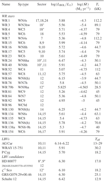
Table 1.List of targets by category, ordered by right ascension (R.A.).
Name Sp.type Sector log(𝐿BOL/𝐿⊙) log( ¤𝑀 ) 𝑇∗
(M⊙yr−1) (kK) WR stars WR 1 WN4s 17,18,24 5.88 –4.3 112.2 WR 3 WN3hw 18∗ 5.56 –5.4 89.1 WR 4 WC5 18∗ 5.71 –4.37 79 WR 5 WC6 18 5.53 –4.59 79 WR 7 WN4s 7 5.36 –4.8 112.2 WR 15 WC6 8,9 5.99 –4.14 79 WR 16 WN8h 9,10 5.72 –4.6 44.7 WR 17 WC5 9,10 5.74 –4.4 79 WR 23 WC6 10 5.61 –4.49 79 WR 24 WN6ha 10∗,11 6.47 –4.3 50.1 WR 40 WN8h 10∗,11 5.91 –4.2 44.7 WR 52 WC4 11 5.07 –4.75 112 WR 57 WC8 11,12 5.75 –4.5 63 WR 66 WN8(h) 12 6.15 –3.9 44.7 WR 78 WN7h 12 5.8 –4.5 50.1 WR 79b WN9ha 12∗ 5.825 –4.565 28.5 WR 81 WC9 12 5.26 –4.62 45 WR 84 WN7 12 5.36 –4.8 50.1 WR 92 WC9 12 4.95 –5 45 WR 96 WC9d 12 WR 130 WN8(h) 14 6.25 –4.2 44.7 WR 134 WN6s 14,15 5.61 –4.4 63.1 WR 135 WC8 14,15 5.4 –4.73 63 WR 136 WN6(h) 14,15 5.78 –4.2 70.8 WR 138a WN8-9h 14,15 5.3 –4.7 40 WR 154 WC6 16,17 5.91 –4.26 79 LBVs 𝑇eff AG Car 10,11 6.14–6.22 13–29 WRAY 15-751 10,11 5.91 30.2 P Cyg 14,15 5.70 18.2 LBV candidates HD 80077 8∗,9∗ 6.30 17.0 2MASS J16493770-4535592 12 𝜁1Sco 12∗ 6.10 18.2 GRS G079.29+00.46 14,15 6.30 25.1 Schulte 12 14,15 6.42 12.9
∗ indicates 2 min cadence data; physical properties come fromNazé et al.(2012, and references therein) for LBVs and candidates, and from the fit results ofSander et al.(2019) for WC stars,
Bohannan & Crowther(1999) for WR 79b,Gvaramadze et al.(2009) for WR 138a, and
Hamann et al.(2019) for other WN stars. The temperature𝑇∗ of Wolf-Rayet stars is defined as the effective temperature related to the stellar luminosity and the stellar radius for an optical depth
𝜏Ross= 20via the Stefan-Boltzmann law (Sander et al. 2019;Hamann et al. 2019).
van der Hucht(2001) and its online extension1 by P.A. Crowther.
To avoid crowding issues, since TESS has a 50% ensquared-energy half-width of 21′′, corresponding to one detector pixel, and since
the photometry is extracted over several pixels, we discarded objects having bright (Δ𝐺 < 2.5 𝑚𝑎𝑔) and close (within 1′) neighbours. Of
the remaining 76 WR stars, only 61 had available TESS photometry. Since we are interested in the intrinsic characteristics of WR stars, we need to avoid contamination by bound companions too. There-fore, we further discarded all objects known to be spectroscopic binaries (SB1 or SB2) as well as those showing some evidence of multiplicity (presence of non-thermal radio emission, dust mak-ing, detected radial velocity shifts). This left 26 WR stars, nearly equally split between WC and WN types, assumed to be single 1 http://pacrowther.staff.shef.ac.uk/WRcat/
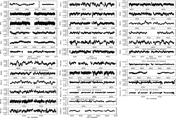
Figure 1.Original lightcurves (in mag) and their long-term trends (in red) which were taken out for subsequent analysis.
(Table1). For all targets but one (WR 96), the physical parameters are known since they were derived using atmosphere modelling by
Sander et al.(2019) for WC stars,Bohannan & Crowther(1999) for WR 79b,Gvaramadze et al.(2009) for WR 138a, andHamann et al.
(2019) for other WN stars.
From the list of LBVs and LBV candidates (cLBVs) from
Nazé et al. (2012), we discarded objects having bright (Δ𝐺 < 2.5 𝑚𝑎𝑔) and close (within 1′) Gaia-DR2 neighbours, as done for
WR stars. Amongst the remaining stars, ten (3 LBVs and 7 candi-dates) were observed by TESS. The multiplicity of LBVs is much less known than for WRs but amongst our targets, two certainly are binaries because they present periodic radial velocity varia-tions and photometric changes: MWC 314 (Richardson et al. 2016) and HD 326823 (Richardson et al. 2011). Having several compo-nents in a target can lead to confusion on the origin of the short-term photometric variability. Indeed, the pulsations detected by
MOSTfor MWC 314 are attributed to its stripped He-star
compan-ion (Richardson et al. 2016). Therefore, we discard those two stars from our target list. Table1provides the final selection, along with their stellar properties taken fromNazé et al.(2012, and references therein).
Note that the presence of very close neighbours is not yet mentioned in Gaia-DR2. However, the Gaia-DR2 available at ESA
Figure 2. TESSlightcurves of the targets (in mag).
archives2 provides a “Renormalised Unit Weight Error” (RUWE,
Lindegren 2016) which should be close to unity if a good fitting of the astrometric observations was achieved by the single star model. For our sample, RUWE is close to one for all stars but WR 66 (RUWE=14), WR 79b (RUWE=3.7), and WR 130 (RUWE=2.7). Furthermore, of the stars listed in Table1, only one (WR 66) pos-sesses a neighbouring component in the Hipparcos catalogue: it is located 0.4′′away from the WR star and is one magnitude fainter
than the latter. Since it passes the chosen criteria, this star is kept in our target list but we remind that some caution should be applied for its results.
2.2 The TESS lightcurves
Launched in April 2018, the TESS satellite (Ricker et al. 2015) pro-vides photometric measurements for ∼85% of the sky. While sky images are taken every 30 min, subarrays on preselected stars are read every 2 min. Observations are available for at least one sector, corresponding to a duration of ∼25 d. The main steps of data reduc-tion (pixel-level calibrareduc-tion, background subtracreduc-tion, flatfielding, and bias subtraction) are done by a pipeline similar to that designed for the Kepler mission.
For 2 min cadence data, time-series corrected for crowding, the limited size of the aperture, and instrumental systematics are
2 https://gea.esac.esa.int/archive/
available from the MAST archives3. We kept only the best quality
(quality flag=0) data. In our sample, only seven stars have such very high cadence data: WR 3, 4, 24 (only sector 10), 40 (only sector 10), 79b, 𝜁1Sco and HD 80077.
For the other stars, individual lightcurves were extracted for each target from TESS full frame images with 30 min cadence. Aper-ture photometry was done on image cutouts of 50×50 pixels using the Python package Lightkurve4. A source mask was defined from pixels above a given flux threshold (generally 10 Median Abso-lute Deviation over the median flux, but it was decreased for faint sources or increased if neighbours existed). The background mask was defined by pixels with fluxes below the median flux (i.e. below the null threshold), thereby avoiding nearby field sources. A prin-cipal component analysis (PCA) then helped correcting the source curve for the background contamination (including scattered light). The number of PCA components was set to five, except for WR 40 and the (c)LBVs where a value of 2 provided better results. All data points with errors larger than the mean of the errors plus three times their 1𝜎 dispersion were discarded. In addition, a few isolated outliers and a few short temporal windows with sudden high scatter were also discarded. For example, for WR 84 and 96, the first hun-dred frames (𝐻𝐽𝐷 < 2 458 627) were affected by a very local and intense patch of scattered light, hence they were discarded.
Whatever the cadence, the raw fluxes were converted into
3 https://mast.stsci.edu/portal/Mashup/Clients/Mast/Portal.html 4 https://docs.lightkurve.org/
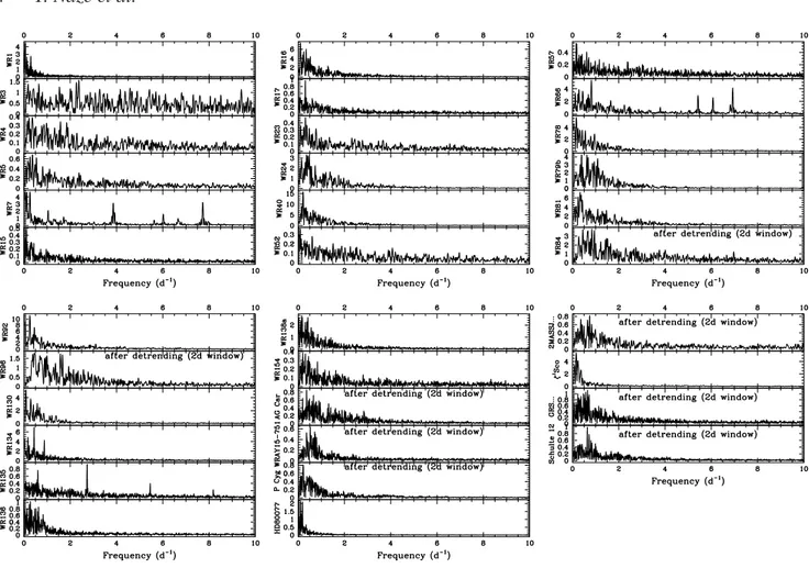
Figure 3.Fourier periodograms associated to the lightcurves shown in Fig.2; the ordinate provides sinusoid amplitudes in mmag (i.e. 𝐴 if the sinusoid has the
form 𝐴 sin(2𝜋𝜈𝑡 + 𝜙)).
magnitudes using 𝑚𝑎𝑔 = −2.5 × log( 𝑓 𝑙𝑢𝑥) and their mean was then subtracted. In several cases, the targets were ob-served over several sectors and the lightcurves were then com-bined. For eight stars (WR 84 and 96, AG Car, WRAY 15-751, P Cyg, 2MASS J16493770-4535592, GRS G079.29+00.46, and Schulte 12), a slow, long-term trend is present in the photometry (Fig.1). As it could impair seeing short-term signals (the goals of this paper), it was determined using a 2 d sliding window and then subtracted. In some cases, the beginning or end of observing windows show a steep upward/downward trend, due to an imper-fect detrending, hence these parts were also discarded. The final lightcurves are shown in Fig.2.
3 RESULTS
The TESS lightcurves of our sample form a varied landscape. The scatter, for example, may take very different values. The lightcurves of LBVs and LBV candidates display scatter of 2 mmag on average, but usually around long-term trends of much larger amplitudes. There is also a clear dichotomy between the WR subtypes. Nine out of the 12 WC-type stars have a scatter less than 2 mmag, and the three remaining stars (WR 81, 92, and 96) are all of the latest, WC9, type. In contrast, all but one (WR 40) WN-type stars have scatter in the 2–14 mmag range, without a clear distinction between early and late types.
All lightcurves were analyzed using a modified Fourier
al-gorithm adapted to uneven temporal samplings (Heck et al. 1985;
Gosset et al. 2001;Zechmeister & Kürster 2009), as there is a small gap in the middle of each sector lightcurve. The periodograms are shown in Fig.3. In addition, to assess the evolution of the variabil-ity pattern, we derived the periodograms in sliding windows of 5 d duration shifted by steps of 0.5 d. These periodograms and the asso-ciated time-frequency diagrams clearly reveal the general presence of red noise, as well as of isolated peaks in a few cases.
3.1 Red noise
The gradual increase in power towards low frequencies in the pe-riodograms, a so-called “red noise”, now appears to be ubiquitous in massive O- and B-type stars (Blomme et al. 2011;Rauw et al. 2019;Bowman et al. 2019b). Such low-frequency variability could be produced by a combination of internal gravity waves excited at the interface between the convective core and the radiative en-velope (Rogers et al. 2013) or in a subsurface convection zone (Blomme et al. 2011). Its presence has also been reported for a few WR stars (Gosset et al. 1990 and more recentlyChené et al. 2011;David-Uraz et al. 2012;Ramiaramanantsoa et al. 2019) but its characteristics were not measured.
Since the pioneering work ofHarvey(1985) linked to “solar noise”, several authors have used formulae of the type 𝑎 + 𝑏
1+(𝑐 𝜈)𝑑
to fit a mixed contribution of white and red noise components. There were however two independent approaches, both of which
we consider below. In all cases, the fitting was performed using a Levenberg-Marquardt algorithm. As a few stars present isolated peaks (see next subsection), these peaks were excised from the periodograms before fitting. The fitting was performed up to 25 d−1
for stars with 30 min cadence lightcurves and up to 360 d−1for stars with 2 min cadence lightcurves. The fitting began at 0.25 d−1 for stars where the lightcurves had been detrended. For WR 24 and 40, lightcurves with 2 min cadence are only available for one sector but we note that the fitted parameters are similar if considering only the 2 min data or the combination of data from both sectors - only the former are presented in Table2.
Whatever the formalism, estimating errors on the derived pa-rameters is not an easy task. The diagonal elements of the variance-covariance matrix at best fit are well known to correspond to squared errors in the linear approximation: we will adopt that formalism, considering that it constitutes a first approximation in our non-linear case. However, it supposes that the fitting is done knowing the error on each input point while there is no formal error on the periodogram amplitudes. To overcome this problem, we may do the fitting without actual errors and consider, as is often done, that the best-fit reduced 𝜒2should amount to one. It should however be mentioned that the periodogram bins are correlated (a peak is spread over several bins and a peak at one place may depend on peaks at other places because of aliasing). The number of degrees of freedom in the frequency space thus does not correspond to the number of points in the fitted periodogram (which is arbitrarily chosen by the user) minus the number of fitted parameters (4). Instead, the actual number of independent frequencies in a periodogram, in the even sampling case, is half the number of points in the lightcurve. There-fore, parameter errors were assumed to be equal to the square root of the diagonal elements of the best-fit variance-covariance matrix, multiplied by the square root of 𝜒2(best fit)/(0.5 × 𝑁data−4) . The
resulting errors are listed in Table2. Note that having performed the fitting in various conditions (different background region masks, fitting of one or two sectors’ data,...) showed that these errors are probably slightly underestimated.
3.1.1 Fitting amplitudes
Brightness variations may be directly related to variations of physi-cal parameters (e.g. 𝑑𝐿/𝐿 ∝ 𝑑𝑇/𝑇), and therefore constitute a prime interest of current asteroseismic studies of massive stars. Therefore, following several recent studies of massive stars (Blomme et al. 2011;Rauw et al. 2019;Bowman et al. 2019b,2020), we may fit the periodogram amplitudes of our targets with:
𝐴(𝜈) = 𝐶 +1 + (2 𝜋 𝜏 𝜈)𝐴0 𝛾 (1)
where 𝐴0is the red noise level at null frequency, 𝜏 the mean lifetime
of the structures producing the red noise, 𝛾 the slope of the linear decrease, and 𝐶 the white noise level.
The fit results are presented in the first part of Table2. For some stars (WR 23, 52, 57, 78, 84, and 134 - for WR 135 the situ-ation is slightly better but 𝐶 remains slightly uncertain), the peri-odogram amplitudes continue to decrease at 25 d−1, i.e. the white noise plateau was not fully reached at that frequency hence we con-sider the fitting as incomplete and do not present its results in Table
2. For a further star (HD 80077), the best-fit appears somewhat in-adequate by eye, with the drop to the white noise level occurring too abruptly; a smaller 𝛾 coupled with a slightly larger 𝐶 provides a better-looking fit, although this “eye-fitting” remains qualitative. Therefore, we prefer not presenting the corresponding fit results.
Table 2.White noise and red noise parameters in TESS data of WR stars and (c)LBVs, each group being ordered by R.A., for each fitting method; the error bars represent ±1𝜎. The number of points in the TESS lightcurves is provided in the last column of the bottom part of this Table.
Amplitude fitting
Star 𝐶 𝐴0 𝜏 𝛾
(mmag) (mmag) (day)
WR1 0.0151±0.0030 2.970±0.091 1.3359±0.0816 1.30±0.04 WR3∗ 0.0189±0.0008 0.572±0.007 0.0140±0.0003 1.84±0.04 WR4∗ 0.0147±0.0002 0.212±0.005 0.0763±0.0034 1.29±0.03 WR5 0.0246±0.0049 0.363±0.029 0.1413±0.0197 1.32±0.15 WR7 0.0323±0.0138 7.170±1.250 2.0701±0.6721 1.02±0.08 WR15 0.0080±0.0018 0.238±0.018 0.3427±0.0543 1.02±0.08 WR16 0.0382±0.0113 3.225±0.114 0.2313±0.0133 1.76±0.10 WR17 0.0219±0.0017 0.277±0.012 0.1552±0.0114 1.61±0.12 WR24∗ 0.0091±0.0005 1.921±0.020 0.1454±0.0024 1.87±0.03 WR40∗ 0.0156±0.0017 6.629±0.072 0.1852±0.0032 1.93±0.03 WR66 0.0888±0.0130 1.756±0.083 0.1120±0.0071 2.38±0.24 WR79b∗ 0.0122±0.0008 1.782±0.018 0.0919±0.0010 3.85±0.12 WR81 0.0514±0.0201 3.537±0.151 0.1476±0.0097 1.84±0.14 WR92 0.0659±0.0250 4.587±0.252 0.2163±0.0194 1.69±0.14 WR96† 0.0647±0.0086 1.145±0.063 0.0976±0.0070 2.08±0.19 WR130 0.0517±0.0089 2.099±0.092 0.2184±0.0135 2.25±0.19 WR135 0.0036±0.0032: 0.299±0.015 0.1199±0.0101 1.20±0.09 WR136 0.0188±0.0014 0.449±0.011 0.1715±0.0054 2.99±0.19 WR138a 0.0419±0.0048 1.492±0.049 0.2377±0.0128 1.75±0.09 WR154 0.0154±0.0012 0.168±0.008 0.1497±0.0122 1.58±0.12 AG Car† 0.0091±0.0021 0.378±0.019 0.1188±0.0083 1.80±0.12 WRAY 15-751† 0.0218±0.0009 0.251±0.009 0.1564±0.0049 4.17±0.37 P Cyg† 0.0106±0.0009 0.373±0.014 0.1783±0.0078 2.33±0.12 2MASS J16493770-4535592† 0.0478±0.0027 0.353±0.024 0.1164±0.0097 2.36±0.27 𝜁1 Sco∗ 0.0246±0.0007 3.990±0.097 0.7199±0.0317 1.32±0.02 GRS G079.29+00.46† 0.0422±0.0023 0.573±0.032 0.1594±0.0115 1.99±0.14 Schulte 12† 0.0135±0.0018 0.332±0.020 0.1353±0.0109 1.91±0.15 Amplitude2 fitting Star 𝑐 𝑎0 𝜏 𝛾 𝑁
(mmag) (mmag) (day)
WR1 1.77±2.12: 1.060±0.052 1.879±0.099 2.11±0.12 3341 WR4∗ 1.07±0.06 0.370±0.002 0.116±0.004 1.81±0.05 14873 WR5 0.76±0.19 0.419±0.014 0.210±0.021 2.28±0.31 1009 WR7 1.19±3.92 2.016±0.211 1.219±0.153 1.98±0.20 1069 WR15 0.39±0.14 0.190±0.009 0.532±0.059 1.74±0.16 1949 WR16 3.58±4.08: 2.717±0.084 0.346±0.019 3.12±0.36 2293 WR17 0.77±0.26 0.317±0.011 0.225±0.020 2.52±0.35 2286 WR24∗ 2.78±1.28: 1.871±0.013 0.215±0.003 4.32±0.18 17575 WR40∗ 3.40±15.4: 6.383±0.083 0.321±0.010 2.41±0.10 17592 WR57 0.51±0.26 0.284±0.009 0.224±0.027 1.66±0.18 2483 WR79b∗ 1.51±3.24 2.445±0.004 0.117±0.002 5.94±0.41 12523 WR81 4.84±2.84: 3.509±0.111 0.237±0.016 3.25±0.47 1247 WR92 5.38±5.01: 3.939±0.175 0.301±0.021 4.21±0.89 1257 WR96† 1.24±1.26 1.569±0.042 0.131±0.010 2.72±0.33 1167 WR130 2.49±2.22: 1.381±0.152 0.582±0.090 2.83±0.74 1201 WR135 0.51±0.32 0.356±0.008 0.173±0.013 2.07±0.20 2370 WR136 0.65±0.51 0.457±0.009 0.208±0.007 5.07±0.64 2364 WR138a 1.28±1.89 1.265±0.035 0.341±0.020 2.54±0.23 2076 WR154 0.58±0.09 0.191±0.005 0.221±0.014 2.73±0.29 2161 AG Car† 0.49±0.49 0.452±0.013 0.165±0.011 2.74±0.29 2400 WRAY 15-751† 0.80±0.15 0.300±0.010 0.185±0.011 3.65±0.48 2072 2MASS J16493770-4535592† 1.04±0.16 0.463±0.013 0.140±0.008 4.38±0.74 1104 𝜁1 Sco∗ 1.85±2.30 1.892±0.025 0.502±0.008 4.02±0.18 12434 GRS G079.29+00.46† 1.61±0.27 0.584±0.005 0.183±0.007 4.63±0.54 2343 Schulte 12† 0.71±0.30 0.367±0.003 0.160±0.009 4.48±0.79 2027
∗ indicates a fitting performed up to 360 d−1, † a fitting beginning at 0.25 d−1, : slight overestimates.
Figure4compares our red noise parameters for 20 single WR stars and 7 LBVs and candidates to those found for 37 O-stars and 29 early B-stars byBowman et al.(2020). As can be seen, the 𝛾 values appear similar for all stars. 𝐴0and 𝜏 may be slightly larger
for evolved stars but the difference is small. The derived similarity in red noise parameters implies that the physical phenomenon re-sponsible for this variability displays similar features in all massive stars. However, in OB-stars, one can directly see the photosphere whereas in WR stars, the hydrostatic surfaces of the stars remain hidden, with the unity optical depth residing inside the wind. On
-3 -2 -1 0 1 0 5 10 15 WR B-stars O-stars LBV -3 -2 -1 0 0 5 10 15 log(C in mmag) 0 0.5 1 1.5 0 5 10 15 20 0 2 4 6 0 5 10 15
Figure 4. Histograms of the white+red noise parameters fitted to peri-odograms of lightcurves from O-stars (dashed blue line, Bowman et al. 2020), B-stars (red dotted line,Bowman et al. 2020), WR stars (black solid line, this work), and (c)LBVs (green long dashed line, Sect. 3.1.1 of this work).
Figure 5.Comparison between the magnitude of the targets and the fitted white noise value (Sect. 3.1.1, top of Table2).
the one hand, the red noise in OB-stars is often considered as the result of internal gravity waves excited by turbulence (either in the convective core or in the near-surface convective layers, see e.g.
Bowman et al. 2020). On the other hand,Ramiaramanantsoa et al.
(2019) demonstrated that a variability similar to that of WR 40 could be produced by a stochastically clumped wind. However, the wind mass loss is directly proportional to the surface radiation flux (Lucy & Abbott 1993;Gräfener et al. 2017) and if it changes due
e.g. to pulsations, then changes in the overlying wind are expected. In particular, a link between wind clumping and perturbations at the level of the hydrostatic radius would not be surprising and our result may possibly be an indirect evidence for it.
In parallel, 𝐶 clearly varies, with B-stars presenting the lowest white noise levels and WRs and (c)LBVs the largest ones - on aver-age, the difference between them amounts to one dex. However, the WR stars of our sample are intrinsically much brighter and/or hot-ter (and the (c)LBVs brighhot-ter) than the OB-stars ofBowman et al.
(2020). Comparing the bright O-type giants and supergiants with the faintest and coolest WR-stars (WR 16, 40, 79b, 81, 92, and 138a), the difference appears less extreme (𝐶 of 4–38 𝜇mag vs 12– 66 𝜇mag). We thus probably observe a continuous trend in white noise levels, driven by temperature and/or luminosity and/or mass-loss effects. A last effect should also be taken into account: the influence of photon noise. Indeed, the intrinsic white noise of the stellar emission is mixed with the photon noise that depends on the apparent magnitude and instrumental sensitivity. In this context, it is interesting to note that lower 𝐶 values can be found for the visu-ally brighter objects while the faintest targets do not display small 𝐶values (Fig.5).
Finally, we checked for correlations between the fitted noise parameters and between them and the stellar properties (Fig.6). This was done for the whole WR sample, but also for WN or WC stars separately. Examining first the noise parameters themselves, the largest Pearson correlation coefficient is found between the noise levels 𝐴0and 𝐶, especially for WC stars (0.5 for the whole sample
but 0.8 for WC). When examining the link with stellar properties, negative correlation coefficients are detected for WC stars between stellar luminosities and both noise levels (coefficients of ∼ –0.9 for 𝐴0and –0.6 for 𝐶), i.e. less noise for intrinsically more
lumi-nous stars. There is also a negative correlation (coefficients of –0.6 for all WR groups) between 𝛾 and stellar temperatures, i.e. slower transitions red→white noise for hotter stars. None of the coeffi-cients are extremely significant, though. In contrast, for OB-stars,
Bowman et al.(2020) found that the red noise level and lifetime 𝜏 (= 1/(2𝜋𝜈char)) decreased towards the ZAMS (i.e. higher
temper-atures and lower luminosities). No obvious correlation appears in the plots for (c)LBVs but given the small number of these targets, it is more difficult to draw general conclusions for them.
In summary, while the red noise parameters of evolved massive stars appear overall similar to those of OB-stars, their relation to stellar properties seems different, possibly more complex.
3.1.2 Fitting squared amplitudes
In the case of data generated by stochastic processes, observed time-series are stochastic entities and so are the associated Fourier and Power Spectra. Following the prescriptions ofDeeming(1975), the combination of stochastic signals (white noise WN, red noise RN) must be performed through the addition of their Power Spectra, i.e. 𝑃(𝜈) = 𝑃WN + 𝑃RN(𝜈). In other words, stochastic processes
sum up quadratically, not linearly, hence a more correct fitting of stochastic processes should actually consider Power Spectra instead of Amplitudes.
A linear process, such as a damped oscillator, excited by a white noise (a general form for a stochastic process) generates time-series whose Power Spectra are proportional to Lorentzian functions, lead-ing to the general expression for the red noise process already men-tioned above. This was the method adopted for granulation studies (Harvey 1985;Kallinger et al. 2014), but also in a cataclysmic
vari-Figure 6.Relationships between red+white noise parameters (Sect. 3.1.1, top of Table2) and bolometric luminosities. Black dots indicate WN stars, blue stars WC stars, and red crosses (c)LBVs.
-1.5 -1 -0.5 0 0.5 1 0 2 4 6 WR LBV -1 -0.5 0 0.5 1 1.5 0 2 4 6 log(c in mmag) 0 0.5 1 1.5 2 0 2 4 6 8 10 0 2 4 6 0 2 4 6
Figure 7.Same as Figs.4and6, but for the squared amplitude fitting.
able analysis (Stanishev et al. 2002) and in one recent massive star analysis (Bowman et al. 2019a).
FollowingKallinger et al.(2014), we therefore consider the sum of the powers:
𝑃(𝜈) = 𝑐2+ 2 𝜋 𝜏 𝜉 𝑃0
1 + (2 𝜋 𝜏 𝜈)𝛾 (2)
where 𝜏, and 𝛾 have similar meanings as before, 𝑐2 and 𝑃 0 are
the white and red noise strengths, and 𝜉 is a normalization factor (Kallinger et al. 2014). Indeed,∫0∞ 𝑑 𝑥
1+𝑥𝛾 = 𝛾sin( 𝜋/𝛾)𝜋 for 𝛾 > 1: to
normalize the integral, a factor 𝜉 = 𝛾
𝜋sin(𝜋𝛾)must then be used. It
ensures that 𝑃0in equation (2) above truly represents all power due
to red noise.
As defined byDeeming(1975),Scargle(1982), andHeck et al.
(1985), power and amplitude are related by 𝑃(𝜈) = 𝑁
4 𝐴2(𝜈)(see
e.g. Sect. II.a ofScargle 1982) where 𝑁 is the number of data points in the lightcurve. The above equation may then be rewritten as:
𝐴2(𝜈) = 4 𝑁𝑐
2+ 2 𝜋 𝜏 𝜉 𝑎20
1 + (2 𝜋 𝜏 𝜈)𝛾 (3)
where 𝑎0is the red noise amplitude.
We thus performed once again the fits, now using the formalism of Eq. (3). The achieved fittings were however of lower quality than in the amplitude-fitting case. In particular, we note that the white noise level is often overestimated: its worse fitting is probably linked to the amplitude squaring which makes its contribution smaller, the fitting procedure then favoring the achievement of a good fit at low frequencies. When the white noise plateau is not reached, its correct determination becomes even more difficult, of course. The
Figure 8.Fourier periodograms showing isolated peaks, with 5 times the red+white noise level (Sect. 3.1.1) marked by the red dotted line. The y-axis provides amplitudes in mmag. The bottom panel provides the typical spectral window for observations in one sector (which is the case of the first three panels) and two sectors (which is the case of the next two panels).
bottom part of Table2thus only lists the fitting results which appear reasonably secure.
As for the previous fitting, we investigated the correlations between parameters derived for WR stars (bottom part of Table2
and right part of Fig.7). Immediately, a strong correlation (Pearson coefficient > 0.9) is found between the two noise levels, confirming the doubts on the white noise level determination. Regarding other parameters, the 𝐴2fitting brings a confirmation to results found in previous subsection: there is an anticorrelation between bolometric luminosities of WC stars and the red noise levels (coefficient of −0.9) as well as an anticorrelation between the slopes and the stellar temperatures (coefficients of −0.5 to −0.7).
Comparing our results for evolved massive stars with typical parameters of OB-stars appears rather difficult as there is only one published study, that ofBowman et al.(2019a). They achieved rea-sonable fittings for only 5 O-stars and 2 early B-stars, although with a different definition of power (that chosen byDegroote et al. 2010). While this prohibits the comparison of noise levels, the 𝜏 and 𝛾 values can still be directly compared (Table2and left part of Fig.7). InBowman et al.(2019a), the slopes 𝛾 of the 7 OB-stars were found to be between 1.8 and 3.3 in all but one case, a range in line with those found here for WR stars. Furthermore, the life-times 𝜏 ranged between 0.06 and 0.14 d−1for OB-stars, on average
somewhat smaller values than for WR stars (where most values lie between 0.1 and 0.35 d−1). Both conclusions are fully in line with
what was derived from the fitting of the amplitude spectra.
3.2 Coherent frequencies
While no (c)LBV shows this feature, five WR stars (i.e. a fifth of our WR sample) display isolated peaks, reminiscent of coherent variability. These stars are WR 7, 66, 79b, 134, and 135 (Fig.8). Assessing their significance requires to take the presence of red
noise into account. Indeed, an overall significance level, derived e.g. from the data scatter (Mahy et al. 2011) or from the mean level outside strong peaks, is valid for all frequencies hence can only be used when the “background” periodogram level does not change with frequency. Therefore, we compared the peak amplitudes to five times the best-fit red+white noise model computed in the Sect. 3.1.15(this corresponds to a signal-to-noise ratio of five at a
prede-fined frequency, as often recommended - see e.g.Baran et al. 2015); no iterative cleaning was performed. The outstanding frequencies are listed in Table3.
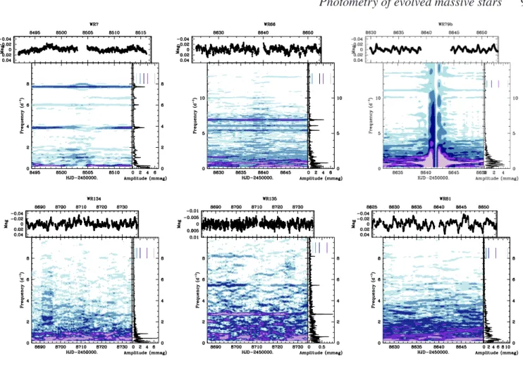
The computed time-frequency diagrams (Fig.9) show that these signals are stable in frequency over the duration of the TESS observations, although their amplitudes may somewhat change. The only exception seems to be WR 134, for which the low-frequency periodogram shows continuous changes. The presence of strong red noise however renders more difficult to assess the stability of the low-frequency signal found for this star. In this context, it is important to note thatMcCandliss et al.(1994),Gosset & Vreux(1996) and
Morel et al.(1999) found a periodicity of 0.44 d−1from line profile variability in spectroscopic datasets of WR 134, a value close to that observed in TESS data: this signal may thus be long-lived.
The peaks appear complex for the one-sector cases (WR 7, 66, and 79b), i.e. peaks are flanked by subpeaks. Such aliases probably arise from the sampling, which notably creates side-lobes at 𝜈peak±0.06 d−1 (Fig.8) - asserting the presence of
ac-tual subpeaks will require a better frequency resolution, i.e. longer lightcurves. What can however already be tested are the relations between frequencies. The main frequencies of WR 7 and those of WR 134 and 135 clearly are harmonics, while additional combina-tions of signals possibly exist in WR 7 (a faint signal near 1.046 is close to the difference between 6.660 and 5.628 d−1) and WR 66 (12.996∼6.076+6.928 d−1). Apart from these, there seems to be no direct relationship (including equal spacing) between signals: WR 7, 66, and 79b thus truly display multiple periodicities.
Several searches for high-frequency signals were performed in the past for WR stars, notably in the context of searches for compact companions (e.g.Marchenko et al. 1994). However, there were few cases of reported and confirmed periodicities. Focusing on our sample, the following detections were published.Blecha et al.
(1992) claimed a detection of pulsations with a 627 s period and a 5 mmag peak-to-peak amplitude in WR 40. However, at the corre-sponding frequency of 138 d−1, the TESS high-cadence data (sector 10) show no sign of such a signal, confirming previous negative reports (Gosset et al. 1994;Marchenko et al. 1994;Martinez et al. 1994;Schneider et al. 1994), including that by the discovery team itself (Bratschi & Blecha 1996). Other low-frequency detections for that star (e.g.Antokhin et al. 1995) certainly correspond to the red noise stochastic variability. Another photometric campaign detected a 6.828 d−1signal in WR 66 (Antokhin et al. 1995) but with strong daily aliasing. It was subsequently confirmed in an independent, less aliased dataset (largest peak at 5.815 d−1Rauw et al. 1996). These values are close (but not identical) to the frequency of the largest
TESSpeak, or its daily alias. To assess the compatibility between
datasets, we have simulated a signal composed of the three main frequencies detected by TESS but sampled as inRauw et al.(1996). The resulting periodogram appears similar to the one reported in
5 The 𝐴2fitting was not used as its quality was lower, especially at high
frequencies. However, we may note that, if adopted, we would reach the same list of significant signals.
Figure 9.Time-frequency diagrams for the five WRs presenting isolated peaks (WR 7, 66, 79b, 134, and 135), compared to the case of WR 81, whose
periodogram only displays red+white noise. The dates in abscissa correspond to the mid-point of the temporal window used for calculating the periodogram. The lightcurve is displayed on top, whilst the periodogram for the full dataset is shown on the right. Short colored lines in the periodogram panels indicate the thresholds used for the colour scheme of time-frequency diagrams.
Table 3.Detected frequencies.
Star Sp.type 𝜈in d−1(ampl. in mmag)
WR 7 WN4s 3.860 (3.14), 5.628 (0.77), 6.020 (1.60), 6.660 (1.00), 7.728∗(3.25)
WR 66 WN8(h) 5.424 (2.94), 6.076 (2.59), 6.928 (4.13), 10.062 (0.52), 12.996 (0.51) WR 79b WN9ha 4.900 (0.28), 10.116 (0.24), 11.096 (0.31), 13.088 (0.22), 13.552 (0.20)
WR 134 WN6s 0.438 (7.01), 0.880∗(4.26)
WR 135 WC8 2.729 (0.93), 5.456∗(0.40), 8.184∗(0.23)
∗ indicates harmonics. Peak widths are 0.04 d−1 for the first three stars (one sector observations) and 0.02 d−1 for the last two (two sector observations); the errors on the peak frequencies are a fraction of that value (typically one tenth). Peak amplitudes from the periodograms are quoted; they are precise to the second decimal as their errors mostly reflect the fluctuations of the local red+white noise levels (see Table6)
which are at 0.10–0.15 mmag for WR 7 and WR 66, 0.01–0.04 mmag for WR79b, 0.6–1.0 mmag for WR 134, and 0.03–0.10 mmag for WR135 (the largest value corresponds to the lowest frequency).
the literature, even if the passbands are different6: the old and new datasets therefore appear fully compatible. Note also that the pres-ence of several frequencies casts further doubt on the hypothesis of the literature signal being the orbital period of a compact compan-ion (Antokhin et al. 1995). Finally, a 25 min signal with 2.6 mmag amplitude was reported byBratschi & Blecha(1996) for WR 78 but considered as a transient event as it was observed only during one
6 Rauw et al.(1996) used Strömgren 𝑏 photometry, which is affected by the
presence of a strong He ii 4686Å line, whereas the TESS passband is larger and redder.
night. Because WR 78 was not observed with 2 min cadence, we cannot check the presence of such a frequency in the TESS data.
Except for WR 134, the detected frequencies are high, from 3 d−1up to 14 d−1. This cannot be easily reconciled with an orbital period (the companion would travel inside the WR star) nor a rota-tion rate (it would be above break-up velocity). Therefore, the most probable culprits are pulsations. WR 66 very probably possesses a close neighbour (see Sect. 2.1), which could cast doubt on the iden-tification of the pulsating star, but that is not the case of the other stars (including WR 123, seeLefèvre et al. 2005). Pulsations here are thus considered to originate from the WR star itself, and such a possibility has actually been considered before. Pushed by the
obser-vational considerations ofVreux(1985), the first pulsation models for WRs were elaborated more than thirty years ago, with predicted periods of about one hour (Maeder 1985;Scuflaire & Noels 1986). Subsequent work byGlatzel et al.(1999) focused on strange modes in small and hot helium stars (often taken as behaving similarly to WRs) and the predicted pulsations had periods of several minutes with amplitudes of several mmag. After the discovery of a 2.45 d−1
signal in WR 123 (Lefèvre et al. 2005), i.e. at a much lower fre-quency than expected, the models were revisited. Strange modes were extended to stars with larger radii (Dorfi et al. 2006;Glatzel 2008) while predictions of g-modes excited by the 𝜅 mechanism were made for WRs byTownsend & MacDonald(2006). In both cases, the predicted periods could be made compatible with the 10 hr signal observed in WR 123. The signals we observe have fre-quencies in the same range, even for the 2 min cadence data, which allows to probe very high frequencies, no coherent signal is detected above 14 d−1: WRs thus seem to pulsate only at moderately high fre-quencies. Furthermore,Townsend & MacDonald(2006) expected pulsations with higher frequencies in early WN (2–8 d−1) than in late WN (1–2 d−1). For our pulsators, only WR 7 has an early WN
type and its frequency values are not particularly higher: its main signals are in the same frequency range as those of the late-type WR 66. Moreover, the highest frequencies are all found in late WN stars. However,Townsend & MacDonald(2006) models were made for “general/typical” stars, not specific ones. In addition, since the WR light mostly comes from inside the wind, the filtering effect by the wind on a signal from the underlying hydrostatic surface needs to be assessed in detail. New, dedicated models will be needed for a more in-depth comparison between observations and predictions.
4 CONCLUSION
In this paper, we aim at characterizing the high-frequency variability of evolved massive stars, either WR stars or LBVs (including LBV candidates). To avoid confusion, we selected only stars not known to be multiple and without bright (Δ𝐺 < 2.5 𝑚𝑎𝑔) and close (within 1′) neighbours in the Gaia-DR2 catalog. Of these, 26 WRs and 8
(c)LBVs had available TESS photometry, with 2 min cadence in 7 cases and 30 min cadence otherwise.
All lightcurves display low-frequency stochastic variability in addition to overall white noise. The parameters of this red noise (level, slope and position of the transition towards white noise) cover a similar range as found for OB-stars byBowman et al.(2020). The white noise level appears larger than in OB-stars, although when focusing on massive stars with similar luminosities and temper-atures, the difference is reduced. Few significant correlations are found, however: as WC stars brighten, the noise levels decrease while the transition red→white noise appears somewhat slower for hotter WRs.
No coherent, isolated signal is found for (c)LBVs, but such signals are detected in five WRs: WR 7, 66, 79b, 134, and 135. WR 134 shows a signal and its first harmonic, WR 135 displays one frequency and its first two harmonics, while the last three stars appear multiperiodic. One frequency in WR 66 and one in WR 134 were reported previously and are thus confirmed by TESS data. Except for WR 134, the detected signals appear at high frequencies (3–14 d−1): such values exclude orbital and rotational modulations, rather favoring a pulsational origin. Our results thus add WR 7, 79b, and 135 to the list of known Galactic high-frequency pulsators which contained up to now WR 66 and 123. Besides, there is no clear trend with WR subtype, unlike what is sometimes predicted
by models. Dedicated modelling is now needed to understand the stellar properties at the hydrostatic surface as well as the exact role of the overlying wind, such as filtering effect and/or additional source of variability.
ACKNOWLEDGEMENTS
The authors acknowledge support from the Fonds National de la Recherche Scientifique (Belgium), the European Space Agency (ESA) and the Belgian Federal Science Policy Office (BELSPO) in the framework of the PRODEX Programme (contracts linked to XMM-Newton and Gaia). They also thank the TESS helpdesk (in particular R.A. Hounsell) for discussion and advices, and D.M. Bowman for discussion. ADS and CDS were used for preparing this document.
DATA AVAILABILITY
The TESS data used in this article are available in the MAST archives.
REFERENCES
Antokhin, I., Bertrand, J.-F., Lamontagne, R., et al. 1995, AJ, 109, 817 Balona, L. A., & Ozuyar, D. 2020, MNRAS, 493, 2528
Baran, A. S., Koen, C., & Pokrzywka, B. 2015, MNRAS, 448, L16 Blecha, A., Schaller, G., & Maeder, A. 1992, Nature, 360, 320 Blomme, R., Mahy, L., Catala, C., et al. 2011, A&A, 533, A4 Briquet, M., Aerts, C., Baglin, A., et al. 2011, A&A, 527, A112 Bohannan, B. & Crowther, P. A. 1999, ApJ, 511, 374
Bowman, D. M., Aerts, C., Johnston, C., et al. 2019a, A&A, 621, A135 Bowman, D. M., Burssens, S., Pedersen, M. G., et al. 2019b, Nature
Astron-omy, 3, 760
Bowman, D.M., Burssens, S., Simón-Díaz, S., et al. 2020, A&A, 640, A36 Bratschi, P. & Blecha, A. 1996, A&A, 313, 537
Chené, A.-N., Moffat, A. F. J., Cameron, C., et al. 2011, ApJ, 735, 34 David-Uraz, A., Moffat, A. F. J., Chené, A.-N., et al. 2012, MNRAS, 426,
1720
Deeming, T. J. 1975, Ap&SS, 36, 137. doi:10.1007/BF00681947 Degroote, P., Briquet, M., Auvergne, M., et al. 2010, A&A, 519, A38 Dorfi, E. A., Gautschy, A., & Saio, H. 2006, A&A, 453, L35
Gaia Collaboration, Prusti, T., de Bruijne, J. H. J., et al. 2016, A&A, 595, A1
Gaia Collaboration, Brown, A. G. A., Vallenari, A., et al. 2018, A&A, 616, A1
Glatzel, W., Kiriakidis, M., Chernigovskij, S., et al. 1999, MNRAS, 303, 116
Glatzel, W. 2008, in proceedings of “Hydrogen-Deficient Stars”, ASP Con-ference Series, Vol. 391, p.307
Godart, M., Simón-Díaz, S., Herrero, A., et al. 2017, A&A, 597, A23 Gosset, E. & Vreux, J. M. 1996, Liege International Astrophysical Colloquia,
33, 231
Gosset, E., Vreux, J.-M., Manfroid, J., et al. 1990, A&AS, 84, 377 Gosset, E., Rauw, G., Manfroid, J., et al. 1994, NATO Advanced Science
Institutes (ASI) Series C, 436, 101
Gosset, E., Royer, P., Rauw, G., et al. 2001, MNRAS, 327, 435 Gräfener, G., Owocki, S. P., Grassitelli, L., et al. 2017, A&A, 608, A34 Gvaramadze, V. V., Fabrika, S., Hamann, W.-R., et al. 2009, MNRAS, 400,
524
Hamann, W.-R., Gräfener, G., Liermann, A., et al. 2019, A&A, 625, A57 Harvey, J. 1985, Future Missions in Solar, Heliospheric & Space Plasma
Physics, 235, 199
Kallinger, T., De Ridder, J., Hekker, S., et al. 2014, A&A, 570, A41. doi:10.1051/0004-6361/201424313
Lefèvre, L., Marchenko, S. V., Moffat, A. F. J., et al. 2005, ApJ, 634, L109 Lenoir-Craig, G., St-Louis, N., Moffat, A. F. J., et al. 2020, Proceedings of the conference Stars and their Variability Observed from Space, 191 Lindegren, L. 2016, Re-normalising the astrometric chi-square in Gaia
DR2, technical note, GAIA-C3-TN-LU-LL-124-01, available from http://www.rssd.esa.int/doc_fetch.php?id=3757412
Lucy, L. B. & Abbott, D. C. 1993, ApJ, 405, 738
McCandliss, S. R., Bohannan, B., Robert, C., et al. 1994, Ap&SS, 221, 155 Maeder, A. 1985, A&A, 147, 300
Mahy, L., Gosset, E., Baudin, F., et al. 2011, A&A, 525, A101
Marchenko, S. V., Antokhin, I. I., Bertrand, J.-F., et al. 1994, AJ, 108, 678 Martinez, P., Kurtz, D., Ashley, R., et al. 1994, Nature, 367, 601 Moffat, A. F. J., Drissen, L., Lamontagne, R., et al. 1988, ApJ, 334, 1038 Moffat, A. F. J., Marchenko, S. V., Lefèvre, L., et al. 2008, Mass Loss from
Stars and the Evolution of Stellar Clusters, 388, 29
Morel, T., Marchenko, S. V., Eenens, P. R. J., et al. 1999, ApJ, 518, 428 Nazé, Y., Rauw, G., & Hutsemékers, D. 2012, A&A, 538, A47 Rauw, G., Gosset, E., Manfroid, J., et al. 1996, A&A, 306, 783 Rauw, G., Pigulski, A., Nazé, Y., et al. 2019, A&A, 621, A15
Ramiaramanantsoa, T., Moffat, A.F.J., Harmon, R., et al. 2018, MNRAS, 473, 5532
Ramiaramanantsoa, T., Ignace, R., Moffat, A. F. J., et al. 2019, MNRAS, 490, 5921
Richardson, N. D., Gies, D. R., & Williams, S. J. 2011, AJ, 142, 201 Richardson, N. D., Moffat, A. F. J., Maltais-Tariant, R., et al. 2016, MNRAS,
455, 244
Ricker, G. R., Winn, J. N., Vanderspek, R., et al. 2015, Journal of Astro-nomical Telescopes, Instruments, and Systems, 1, 014003
Rogers, T.M., Lin, D.N.C., McElwaine, J.N., & Lau, H.B.B. 2013, ApJ, 772, 21
Sander, A. A. C., Hamann, W.-R., Todt, H., et al. 2019, A&A, 621, A92 Scargle, J. D. 1982, ApJ, 263, 835. doi:10.1086/160554
Schmutz, W. & Koenigsberger, G. 2019, A&A, 624, L3
Schneider, H., Kiriakidis, M., Weiss, W. W., et al. 1994, Pulsation; Rotation; and Mass Loss in Early-Type Stars, 162, 53
Schneider, H., Glatzel, W., & Fricke, K. J. 1997, Luminous Blue Variables: Massive Stars in Transition, 120, 206
Scuflaire, R. & Noels, A. 1986, A&A, 169, 185
Stanishev, V., Kraicheva, Z., Boffin, H.M.J., & Genkov, V. 2002, A&A, 394, 625
Sterken, C. & Breysacher, J. 1997, A&A, 328, 269
Townsend, R. H. D. & Owocki, S. P. 2005, MNRAS, 357, 251 Townsend, R. H. D. & MacDonald, J. 2006, MNRAS, 368, L57 van der Hucht, K. A. 2001, New Astron. Rev., 45, 135 Vreux, J.-M. 1985, PASP, 97, 274
Zechmeister, M. & Kürster, M. 2009, A&A, 496, 577