HAL Id: pastel-00563352
https://pastel.archives-ouvertes.fr/pastel-00563352
Submitted on 4 Feb 2011HAL is a multi-disciplinary open access archive for the deposit and dissemination of sci-entific research documents, whether they are pub-lished or not. The documents may come from teaching and research institutions in France or abroad, or from public or private research centers.
L’archive ouverte pluridisciplinaire HAL, est destinée au dépôt et à la diffusion de documents scientifiques de niveau recherche, publiés ou non, émanant des établissements d’enseignement et de recherche français ou étrangers, des laboratoires publics ou privés.
Nitrogen fluxes in a perennial energetic crop,
Miscanthus x giganteus : experimental study and
modelling elements
Strullu Loïc
To cite this version:
Strullu Loïc. Nitrogen fluxes in a perennial energetic crop, Miscanthus x giganteus : experimental study and modelling elements. Agronomy. AgroParisTech, 2011. English. �NNT : 2011AGPT0001�. �pastel-00563352�
INRA
présentée et soutenue publiquement par
Loïc STRULLU
Le 06/01/2011
Flux d’azote dans une culture pérenne à vocation énergétique,
Miscanthus x giganteus : étude expérimentale et éléments de modélisation
Doctorat ParisTech
T H È S E
pour obtenir le grade de docteur délivré par
L’Institut des Sciences et Industries
du Vivant et de l’Environnement
(AgroParisTech)
Spécialité : Agronomie
Directeur de thèse : Marie-Hélène JEUFFROY
Co-encadrement de la thèse : Nicolas BEAUDOIN et Stéphane CADOUX
Jury
M. Benoit GABRIELLE, PR, UMR EGC, INRA/AgroParisTech Président
M. François GASTAL, DR, URP3F, INRA Rapporteur 1
M. Christophe SALON, DR, UMR LEG, INRA/ENESAD Rapporteur 2
M. Ghislain GOSSE, DR, DR honoraire, INRA Examinateur
M. Gianpetro VENTURI, PR, Agronomy and Industrial Crops, DISTA-GRICI Examinateur
M. Francis VALTER, Ingénieur, Sofiproteol Examinateur
La fin de la thèse est proche et il est grand temps de remercier tous les acteurs qui ont participé à la réalisation de ce travail.
Je tiens tout d’abord à remercier les chercheurs et ingénieurs de l’unité Agro-Impact qui ont bien voulu me confier ce travail. Je tiens également à les remercier pour les connaissances en agronomie et sur les impacts environnementaux associés aux cultures qu’ils ont su me transmettre.
Marie-Hélène Jeuffroy a dirigé cette thèse et je lui suis grandement reconnaissant pour son implication dans la thèse malgré notre éloignement géographique. Elle a su se rendre disponible quand cela était nécessaire, notamment lors de la rédaction des différents articles pour partager son expertise.
Mes encadrants, Nicolas Beaudoin et Stéphane Cadoux, ont su me laisser suffisamment de liberté pour que je puisse m’approprier ce travail tout en suivant le déroulement du projet afin d’éviter que je ne m’égare et ne m’épuise dans des considérations secondaires. Leur aide a été précieuse tout au long de cette expérience professionnelle et je les en remercie.
Viennent ensuite les membres du comité de pilotage de thèse (Jean-Louis Durand, Maryse Brancourt, Frédéric Dubois, Francis Valter et Hubert Boizard notre directeur d’unité), qui ont apporté un regard extérieur sur la thèse et qui m’ont permis, de par leurs interrogations et remarques, de mieux cerner et expliciter ma problématique de thèse.
La partie expérimentale a été un très gros morceau de cette thèse. Je n’ai pas réalisé les expérimentations sur M. giganteus seul, l’équipe « Biomasse et Environnement » de l’unité a toujours répondu présente quand j’avais besoin d’aide. Je tiens tout particulièrement à remercier Emilie Fourdinier, sans qui je n’aurais pas pu faire la moitié des expérimentations. Sa bonne humeur, sa volonté, sa rigueur et son désir du travail bien accompli ont rendu mon travail bien plus simple et agréable. Matthieu Predhomme, qui a maintenant quitté l’unité, a également pris du temps pour m’aider dans mes expérimentations, en plus de son travail d’ingénieur, et je lui en suis très reconnaissant. Savoir qu’ils étaient là tous les deux et qu’ils répondraient toujours présents si j’avais besoin d’aide, m’a permis d’effectuer les expériences nécessaires à la réalisation de cette thèse.
Je tiens également à remercier Julie Haxaire, une stagiaire de Licence, qui a effectué un travail remarquable afin de déterminer le coefficient d’extinction des rayonnements par une
pas les faire seul. Frédéric Mahu, qui m’a expliqué le fonctionnement du LAI-2000 et des centrales d’acquisitions automatiques de données. Jean-Luc de l’Unité Expérimentale d’Estrées-Mons qui a bien voulu nous prêter sa force pour les prélèvements au combien fatigants des rhizomes de miscanthus.
Charlotte Demay, ingénieur d’étude, toujours (ou presque) de bonne humeur et souriante, je te remercie pour toute l’aide que tu m’as apporté au niveau expérimental mais surtout pour les moments « pause-café-clope-blabla » si importants pour l’équilibre mental d’un thésard. Hélène Zub, ex-thésarde et aujourd’hui Docteur, avec qui j’ai partagé pendant deux ans mon bureau, je te remercie pour le soutien moral que tu m’as apporté pendant ma thèse et pour le partage de ton expertise sur miscanthus que tu avais rencontré et commencé à étudier avant moi. Olivier Postaire, post-doc, situé dans le bureau d’en face, avec qui j’ai souvent discuté de cette culture nouvelle qu’est le miscanthus et dont les discussions m’ont amené à réfléchir et à clarifier mes idées.
Enfin, je remercie tous les membres de l’Unité Agro-Impact qui ont su se mobiliser lors des « opérations coup de poing » nécessaires à la mise en place des capteurs de rayonnements. Je remercie également les membres de l’Unité Expérimentale pour le temps consacré à la fabrication de socles et autres mats nécessaires au positionnement des capteurs de rayonnements dans les parcelles de miscanthus.
Pour les moments de détente, je remercie tous les collègues qui se rassemblent tous les midis pour aller manger puis jouer au babyfoot ou au ping-pong.
Introduction et Problématique 1
Objectifs et Plan de la thèse 9
Chapitre 1: Biomass production, nitrogen accumulation and remobilisation by
Miscanthus x giganteus as influenced by nitrogen stocks in belowground organs 12
Abstract 12
Keywords 13
1. Introduction 14
2. Materials and methods 16
2.1. Experimental site and trial setup 16
2.2. Biomass sampling 16
2.3. Nitrogen analysis 18
2.4. Calculation of nitrogen content 19
2.5. Calculation of apparent nitrogen fluxes 19
2.6. Data analysis 21
3. Results 23
3.1. Biomass production of Miscanthus x giganteus. effect of harvest date and nitrogen
fertilisation 23
3.2. Nitrogen concentration in aboveground and belowground biomass: effect of
harvest date and nitrogen fertilisation 24
3.3. Nitrogen accumulation and partitioning between aboveground and belowground plant parts : effect of harvest date and nitrogen fertilisation 25 3.4. Nitrogen fluxes within the plant : spring and autumn remobilisation 27
3.5. Soil-crop relationship 28
4. Discussion 30
4.1. Nitrogen accumulation and partitioning in Miscanthus x giganteus: effect of
nitrogen stocks and fertilisation 30
4.2. Soil-crop relationship 31
4.3. Spring remobilisation 32
4.4. Autumn remobilisation 33
5. Conclusions 37
Acknowledgements 38
References 39
Chapitre 2: Influence of belowground nitrogen stocks on light interception and conversion by Miscanthus x giganteus 42
Abstract 42
Keywords 42
1. Introduction 43
2. Materials and methods 45
Study site and trial set-up 45
Biomass sampling 45
Kinetics of LAI development 47
Determination of the extinction coefficient and εior εa max 47
Determination of radiation use efficiency, RUE 48
Nitrogen analysis and calculation of N content 49
Data analysis 49
3. Results and discussion 50
3.1. Radiation interception 50
Leaf Area Index development 50
Leaf Area Index growth rate 51
PAR interception and absorption by the crop 52
Effect of nitrogen on LAI development 53
3.2. Radiation use efficiency of M. giganteus 55
4. Conclusions 57
Acknowledgements 57
References 58
Chapitre 3 : Assessment of nitrogen absorption and remobilisation using 15N-labelled in
Miscanthus x giganteus with early or late harvest date 61
Abstract 61
Keywords 61
N content 66
Stastistical analysis 66
3. Results 67
3.1. Biomass production 67
3.2. Nitrogen content and 15N recovery in plants 67 3.2.1. Nitrogen content in aboveground organs 67 3.2.2. Nitrogen content in belowground organs 68
3.2.3. Nitrogen content in the whole crop 69
3.3. Nitrogen rough fluxes within the plant 69
3.3.1. Rough N fluxes occurring during plant growth 69
3.3.2. Daily N fluxes 70
3.3.3. Cumulated N fluxes 70
3.3.4. N cycling 71
3.3.5. 15N recovery uncertainties 72
4. Discussion 73
4.1. Biomass production and N content at harvest 73
4.2. Recovery of 15N-labelled fertilized 73
4.3. N fluxes within the crop 74
4.3.1. N absorption 74 4.3.2. N remobilisation 75 5. Conclusion 77 Acknowledgements 77 Appendix 78 References 82
Chapitre 4 : Discussion des résultats et éléments de modélisation du fonctionnement
pluriannuel de la culture 84
1. Introduction 84
2. Variabilité de la biomasse des organes souterrains et conséquences 84 3. Dynamique de l’azote à moyen et long terme dans une culture de Miscanthus x
giganteus 85
5.1. Indicateur de nutrition 89 5.2. Fonction de stress « azote » sur la mise en place de l’indice foliaire 90 5.3. Fonction de stress N sur la production de biomasse par la culture 91
5.4. Conclusion sur le modèle conceptuel 91
Conclusion et perspectives 93
INTRODUCTION
Figures
Figure 1: Schéma du fonctionnement d’une culture de M. giganteus à partir de la
bibliographie de l’introduction.
CHAPITRE 1
Figures
Figure 1: Monthly rainfall and temperature during the two years of Miscanthus x giganteus
growth studied (2008 and 2009).
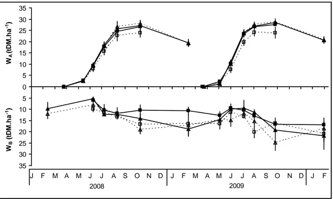
Figure 2: Effect of harvest date and fertilisation on aboveground and belowground biomass
production of Miscanthus x giganteus in the third and fourth years of growth.
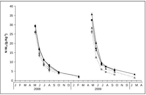
Figure 3: Nitrogen concentration (a) in aboveground biomass and (b) in belowground
biomass during the two years of growth.
Figure 4: Effect of harvest date and fertilisation on aboveground and belowground nitrogen
content of Miscanthus x giganteus in the third year and fourth years of growth.
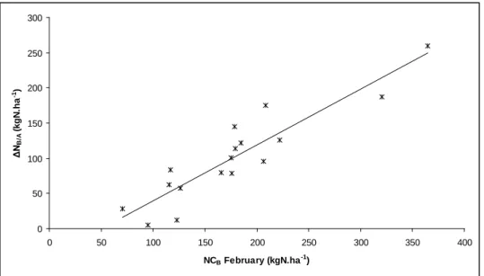
Figure 5: Relationship between spring remobilisation (ΔNB/A = kgN.ha-1) calculated with
equation (6) and initial nitrogen stocks in belowground biomass (kg N ha-1).
Figure 6: Relationship between autumn remobilisation (ΔNA/B = kgN.ha-1) calculated with
equation (7) and maximum nitrogen accumulation in aboveground biomass (kgN.ha-1).
Figure 7: Relationship between the aboveground biomass nitrogen accumulation rate
(kgN.ha-1.dd-1) of the crop and the belowground biomass nitrogen stocks before regrowth (kgN.ha-1).
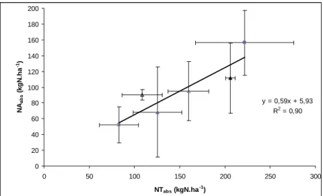
Figure 8: Relationship between the nitrogen taken up recovered in aboveground plant parts
(NAabs = kgN.ha-1) and nitrogen uptake by the whole crop (NTabs = kgN.ha-1).
Tableaux
Table 1: Spring remobilisation (ΔNB/A = kgN.ha-1) from belowground to aboveground
biomass calculated in two successive years (± standard error) and its relative contribution to aboveground biomass nitrogen accumulation (%).
Table 2: Autumn remobilisation from aboveground to belowground biomass (ΔNA/B =
kgN.ha-1) calculated in two successive years (± standard error).
Table 3: Soil mineral nitrogen in the 0-150 cm layer (± standard error) at the end of winter in
CHAPITRE 2
Figures
Figure 1: Leaf area index (LAI) development of M. giganteus as a function of degree-days
(oC) in a) the third year of growth (2008) and b) the fourth year of growth (2009) in the various treatments.
Figure 2: Relationship between maximum leaf area index growth rate (MLGR) and
belowground nitrogen stocks before regrowth (NCB, kgN.ha-1).
Figure 3: Relationship between leaf area index (LAI) and radiation interception efficiency by
the canopy.
Figure 4: Relationship between leaf area index (LAI) and aboveground N uptake (NCA) in a)
the third year of growth (2008) and b) the fourth year of growth (2009).
Figure 5: Relationship between aboveground biomass (WA) and cumulative
photosynthetically active radiation (PAR) intercepted by the crop from emergence to the beginning of senescence in a) the third year of growth (2008) and b) the fourth year of growth (2009).
Figure 6: Relationship between radiation use efficiency (RUE, g.MJ-1) determined from intercepted photosynthetically active radiation (PAR) and belowground nitrogen stocks (NCBi) before regrowth (kgN.ha-1).
Tableaux
Table 1: Monthly water balance (P – ET0, mm) and cumulative deficit between April and
August in 2008 and 2009.
Table 2: Maximum leaf area index growth rate (MGLR = m2.m-2.dd-1) calculated in the
different treatments during the two years of growth.
Table 3: Photosynthetically active radiation (PAR) intercepted by Miscanthus x giganteus
determined before nitrogen remobilisation between aboveground and belowground biomass.
Table 4: Nitrogen use efficiency for leaf area index development (NUELAI) in the different
treatments during two years of growth and correlation coefficient for the linear regression.
Table 5: Intercepted or absorbed photosynthetically active radiation (PAR) and radiation use
efficiency (RUE) of Miscanthus x giganteus, determined before nitrogen remobilisation between aboveground and belowground biomass.
CHAPITRE 3
Figures
Figure 1: Time-course change in nitrogen content (NC), 15N excess and N uptake from fertilization (NCf) a) in the aboveground biomass (A), left column; b) in the belowground
Tableaux
Table 1: Biomass production of Miscanthus x giganteus in the different organs of the plant, at
different dates.
Table 2: 15N partitioning, as percentage of total 145N-labelled fertilizer uptake by the whole crop, in the aboveground and belowground organs of the crop, at different dates, for early (autumn) and late (February) harvests.
Table 3: 15N recovery (%) in Miscanthus x giganteus in the aboveground and belowground organs of the crop, at different dates, for early (autumn) and late (February) harvests.
Table 4: Mean daily nitrogen fluxes per period within the plant (kgN ha-1 d-1).
CHAPITRE 4
Figures
Figure 1: Evolution de l’azote minéral du sol dans les 0-150 cm depuis l’implantation de la
culture de Miscanthus x giganteus en avril 2006.
Figure 2: Evolution des réserves en azote contenues dans les organes de réserve de M.
giganteus au cours des deux années d’expérimentation.
Figure 3: Evolution de la quantité d’azote dans les plantes entières au cours des deux années
d’expérimentation.
Figure 4: Schéma du fonctionnement d’une culture de M. giganteus à partir des résultats de
Introduction
&
L’atténuation des changements climatiques, et la sécurisation sur le long terme, des
approvisionnements énergétiques, sont des défis majeurs du XXIème siècle. Le rapport du
Groupement Intergouvernemental des Experts sur le Climat (GIEC) de 2007 met en avant
l’implication de l’augmentation des gaz à effet de serres (GES) d’origine anthropique dans le
réchauffement climatique observé depuis la moitié du XXème siècle. Au niveau mondial, les
principales sources de GES d’origine anthropique (en particulier CO2, N2O et CH4) des
secteurs d’activité économique sont : la production d’électricité, l’industrie, l’agriculture et les
transports (Stern, 2006). Dans ce contexte, et pour se conformer au protocole de Kyoto,
l’Union Européenne a décidé de promouvoir l’utilisation d’énergies produites à partir de
ressources renouvelables (énergie éolienne, solaire, biomasse, etc.). La Directive Européenne
2009/28/CE a fixé pour objectif aux états membres d’atteindre 20% la part d’énergie
renouvelable dans la consommation finale brute d’énergie de la Communauté d’ici à 2020.
Elle impose également une part minimale de 10% de biocarburants dans la consommation
totale d’essence et de gazole destinés au transport, mais fixe des critères de durabilité à
respecter. D’après la directive, les biocarburants doivent permettre de réduire d’au moins 35%
les émissions de GES par rapport aux carburants d’origine fossile, avec un objectif de 60% à
partir de 2018. De plus, la directive exclut certaines situations pour la production de cultures
destinées à la fabrication de biocarburants, comme les prairies naturelles, les forêts primaires
ou les zones humides.
En 2009, la part des énergies renouvelables représentait 8.1% de la consommation finale
d’énergie en France (Service de l’observation et des statistiques, 2010). Les objectifs à 2020
pour la France, fixés par la directive européenne, sont de porter cette part à 23%. Pour
diminuer ses émissions de GES, la France s’est notamment tournée vers les biocarburants car
le secteur des transports est le premier secteur émetteur de GES en France du fait de son
des énergies renouvelables (2009-2020), la France prévoit que les biocarburants
représenteront la majeure partie des énergies renouvelables dans la consommation d’énergie
finale brute d’ici à 2020.
Les biocarburants actuels, produits à partir de parties de plantes utilisées initialement pour
la production alimentaire (biocarburants de 1ère génération), soulèvent de nombreuses
inquiétudes sur les bilans nets d’énergie et de gaz à effet de serre et sur la compétition
potentielle avec les productions alimentaires (FAO, 2008). La possibilité d’utiliser la
ligno-cellulose pour la production de biocarburants (biocarburants de 2ème génération) offre la
perspective d’ouvrir le panel des ressources candidates (déchets urbains et industriels,
coproduits agricoles et forestiers, cultures pérennes dédiées, etc.) et de trouver des cultures
mieux adaptées pour faciliter la réponse au « trilemme alimentation, énergie, environnement »
(Tilman et al., 2009). L’utilisation de cultures dédiées pour la fabrication de biocarburants de
2ème génération ne sera acceptable qu’à condition de limiter les impacts des pratiques
agricoles qui leur sont appliquées, au niveau global (émissions de GES), mais aussi local
(lixiviation des nitrates ou de pesticides, consommation en eau, etc.). Les plantes candidates
devront donc répondre à ces exigences tout en alliant un rendement élevé à l’hectare, afin de
limiter la concurrence entre productions alimentaires et non alimentaires (Sims et al., 2006).
En effet, le développement des biocarburants conduira à l’utilisation de terres agricoles
jusqu’ici dédiées à la production de nourriture. Plus une culture sera productive, moins la
pression sur les terres arables sera forte.
Au vu des exigences citées précédemment, Miscanthus x giganteus apparaît être l’une des
cultures les plus prometteuses pour fournir la matière première pour la fabrication de
biocarburants de 2ème génération (Somerville et al., 2010). M. giganteus, originaire d’Asie du
Coupe précoce (mi-octobre)
sinensis. Il est étudié depuis les années 80 en Europe pour son intérêt comme culture énergétique. C’est une plante pérenne en C4, appartenant à la famille des Poaceae, au
potentiel de production élevé. La première année démarre par la plantation de morceaux d’un
rhizome mère. Jusqu’aux premières gelées, la plante s’installe et développe principalement
ses organes souterrains (Beale and Long, 1995). La culture est broyée en fin d’hiver de
l’année d’implantation car la production de biomasse aérienne est très limitée. En Europe, le
rendement de M. giganteus peut atteindre, à partir de la deuxième année de culture, 20 à 50
tMS.ha-1.an-1 quand la récolte a lieu en automne (récolte précoce) et 10 à 30 tMS.ha-1.an-1
quand la récolte a lieu fin d’hiver (récolte tardive) (Clifton-Brown et al., 2000 et 2004 ; Tayot
et al., 1994). Si le rendement est supérieur lors d’une récolte précoce, les teneurs en éléments minéraux, notamment en azote, et en eau sont plus faibles lors de la récolte tardive
(Lewandowski and Heinz, 2003). Pour la production de biocarburants de 2ème génération,
deux voies très différentes sont envisagées : la voie fermentaire ou voie humide, et la voie
thermochimique ou voie sèche. L’efficacité des voies fermentaires dépend des composants de
la paroi des cellules végétales (cellulose et hémicellulose) et de leur récalcitrance à la
dégradation. L’efficacité des voies thermochimiques est liée, quant à elle, à des taux
d’humidité et des contenus en cendres et éléments minéraux faibles (Karp and Shield, 2008).
Selon la voie de transformation, et donc les critères de qualité de la biomasse qui sont
attendus, l’une ou l’autre des stratégies de récolte du miscanthus pourrait être préférable.
Pour tout couvert végétal, la contribution de l’azote à l’élaboration de la biomasse est un
élément majeur car i) l’azote est un facteur de croissance essentiel pour la plante (rôle clé sur
le développement de l’indice foliaire et la production de biomasse), ii) l’utilisation d’engrais
azotés a un impact fort sur le bilan énergétique, du fait du procédé de synthèse (Lewandowski
de N2O et/ou NH3 (Crutzen et al., 2008) ou des pertes de NO3 par lessivage (Beaudoin et al.
2005). Différentes études ont été menées en Europe afin de déterminer les réponses d’une
culture de M. giganteus à un apport d’azote, mais leurs résultats sont contradictoires. Des
expérimentations ont montré un effet positif de la fertilisation azotée sur la production de
biomasse par une culture de M. giganteus récoltée précocement (Ercoli et al., 1999 ; Acaroglu
et al., 2005), ou tardivement (Cosentino et al., 2007 ; Boehmel et al., 2008). Cependant, d’autres études concluent à l’absence d’effet de la fertilisation azotée sur la production de
biomasse par une culture de M. giganteus récoltée tardivement (Beale et al., 1996 ; Himken et
al., 1997 ; Clifton-Brown et al., 2007 ; Christian et al., 2008). Cette absence de réponse à la fertilisation azotée, ou les faibles besoins de cette culture en fertilisation azotée (Beale et
Long, 1997 ; Himken et al., 1997 ; Lewandowski et al., 2000), peuvent s’expliquer par
différentes caractéristiques, à commencer par une efficience d’utilisation de l’azote très
élevée, qui varie entre 190 gMSA.gN-1 et 350 gMSA.gN-1 (Consentino et al., 2007 ;
Lewandowski and Schmidt, 2006). Ces valeurs sont supérieures aux valeurs habituellement
observées pour les plantes annuelles en C3 (Lewandowski and Schmidt, 2006). D’autre part, à
l’automne et pendant l’hiver, M. giganteus recycle une partie de l’azote accumulé pendant la
croissance via la chute des feuilles et la mise en réserve de l’azote contenu dans les organes
aériens vers les organes souterrains. L’azote issu de la chute des feuilles pourra être
disponible pour la culture, les années suivantes, après minéralisation. Une partie de l’azote
stocké dans les rhizomes est remobilisée au printemps, diminuant ainsi les besoins en azote
externe (Beale and Long 1997 ; Himken et al., 1997, Kahle et al., 2001). Enfin, Eckert et al.
(2001) ont isolé une bactérie du genre Azospirillum associée aux racines d’une culture de M.
giganteus âgée de 5 ans en Allemagne, Azospirillum étant un genre constitué de bactéries endophytes facultatives, capables de fixer l’azote atmosphérique (Steenhoudt et al., 2000).
l’automne puis remobilisation au printemps et possible fixation d’azote atmosphérique), sont
à l’origine de la faible réponse et/ou l’absence de réponse à la fertilisation azotée observée
chez M. giganteus lors d’une récolte en coupe tardive (Cadoux et al. submitted).
L’effet de la date de coupe sur la production de biomasse et sur la nutrition azotée de la
plante par une culture de Miscanthus x giganteus n’a, à notre connaissance, jamais été étudié.
Or une coupe précoce en automne, lorsque la production de biomasse par la culture est
maximale empêche la chute des feuilles et pourrait limiter tout ou partie de la mise en réserve
des nutriments, notamment l’azote. Différentes études sur les plantes pérennes comme les
arbres (Millard and Grelet, 2010), la luzerne (Avice et al, 1996 ; Teixeira et al, 2007 ; Ourry
et al., 1994) ou les graminées fourragères (Thornton and Millard, 1997; Louahlia et al., 1999), montrent que les réserves azotées ont un rôle primordial sur la nutrition azotée et la croissance
de la plante lors du redémarrage de la culture au printemps et donc sur la production de
biomasse. En effet, les réserves en azote influent sur la mise en place de l’indice foliaire des
plantes (Avice et al., 1996 ; Thornton and Millard, 1997 ; Teixeira et al., 2007) ainsi que sur
leur efficience de conversion des rayonnements (Avice et al., 1996). Il semble donc important
de comprendre les implications d’une coupe précoce, potentiellement intéressante pour des
voies de valorisations fermentaires, et plus largement de comprendre les déterminants des flux
de remobilisation ainsi que leur implication dans le fonctionnement de la plante.
Différents auteurs ont montré que l’efficience d’utilisation des rayonnements et la vitesse
de mise en place de l’indice foliaire dans une culture de M. giganteus augmentaient avec
l’âge de la culture pendant la phase d’installation, notamment entre la 1ère et la 3ème année de
culture (Cosentino et al., 2007 ; Jørgensen et al., 2003). Cependant, aucune étude à ce jour n’a
compréhension des déterminants des flux d’azote au sein de la plante, notamment les flux de
remobilisation de l’azote, rend difficile la compréhension et la prévision des besoins en azote
externe à apporter à la culture.
La modélisation fournit un outil puissant pour étudier la production de biomasse actuelle
et potentielle d’une culture dans différentes conditions, et peut également être utilisée pour
tester différentes hypothèses sur l’effet de l’altération de caractéristiques physiologiques et/ou
phénotypiques ainsi que les effets du changement climatique. Les modèles
sol-plante-atmosphère permettent également la simulation des impacts environnementaux liés à l’eau,
l’azote et l’énergie (Brisson et al., 1998) et peuvent donc être utilisés pour aider au choix des
plantes les mieux adaptées au débouché bioénergie en prenant en compte les différents
critères recherchés. Les modèles empiriques sont utiles pour aider à prédire le rendement
d’une culture dans différents contextes climatiques, cependant, les modèles mécanistes sont
plus informatifs quant aux processus impliqués dans la croissance de la plante. A ce jour, il
n’y a pas de modèle mécaniste prenant en compte la dynamique de l’azote entre la partie
aérienne de la plante et sa partie souterraine pour les plantes dédiées à la production de
biomasse. Toutefois, différents modèles permettant de simuler la production de biomasse par
une culture de M. giganteus ont été paramétrés et publiés. Le premier modèle publié est un
modèle empirique simulant la production potentielle : MISCANMOD (Clifton-Brown et al.,
2000). Ce modèle n’intègre ni les effets des stress hydriques et/ou azotés, ni les réserves
contenues dans les rhizomes. Ce modèle a ensuite été amélioré en intégrant de nouvelles
connaissances sur la physiologie de la plante et en prenant en compte l’effet d’un stress
hydrique sur la production de biomasse ainsi que l’effet de la température: MISCANFOR
(Hastings et al., 2009). MISCANFOR présente donc une avancée importante, mais il ne
Dormance Stock initial de C & N Emergence Remobilisation N 23 à 55 kgN.ha-1 Absorption N & Allocation Mise en réserve N 45 à 101 kgN.ha-1
Indice foliaire Coefficient d’extinction des rayonnements (0.56 à 0.68) Rayonnements interceptés RUE
(1.1 à 4.0 gMS.MJ-1)
Biomasse
Sénescence Allocation de C aux
organes souterrains à l’aide d’un coefficient de partition
Chute des feuilles 68 à 111 kgN.ha-1
Phase de croissance
Figure 1:Schéma du fonctionnement d’une culture de M. giganteus à partir de la bibliographie de l’introduction. Dormance Stock initial de C & N Emergence Remobilisation N 23 à 55 kgN.ha-1 Absorption N & Allocation Mise en réserve N 45 à 101 kgN.ha-1
Indice foliaire Coefficient d’extinction des rayonnements (0.56 à 0.68) Rayonnements interceptés RUE
(1.1 à 4.0 gMS.MJ-1)
Biomasse
Sénescence Allocation de C aux
organes souterrains à l’aide d’un coefficient de partition
Chute des feuilles 68 à 111 kgN.ha-1
Phase de croissance
que de manière très simplifiée, au travers d’un indicateur basé sur le niveau de fertilisation
azotée. Un autre modèle a été récemment paramétré pour M. giganteus : WIMOVAC (Miguez
et al., 2009). Ce modèle fonctionne à partir de la simulation de la photosynthèse au niveau du peuplement végétal et les assimilats carbonés sont ensuite distribués dans les différents
organes de la plante en fonction du stade de développement de la culture. Ce modèle prend en
compte les rhizomes en intégrant les flux de carbone entre partie aérienne et souterraine à
l’aide d’un coefficient de partition du carbone assimilé, mais il n’intègre pas les flux d’azote
entre parties aériennes et souterraines.
L’ensemble des connaissances issues de la bibliographie nous permet de proposer un
schéma conceptuel du fonctionnement de M. giganteus présentant les principaux processus ou
paramètres connus et ceux à déterminer pour la modélisation de la plante (Figure 1).
L’approche de la production de biomasse basée sur l’efficience d’interception et de
conversion du rayonnement lumineux (Monteith et al., 1977) semble a priori adaptée au
miscanthus. Ainsi, pour modéliser la production de biomasse par la culture, il est nécessaire
de simuler le développement de l’indice foliaire et de déterminer le coefficient d’extinction de
la culture afin de pouvoir simuler l’interception des rayonnements par le peuplement végétal.
Les rayonnements interceptés seront convertis en biomasse en fonction d’une efficience de
conversion. Il faut ensuite déterminer la partition des assimilats carbonés dans la plante entre
partie aérienne et partie souterraine, comme suggéré par Miguez et al. (2009), en prenant en
compte la phase d’entrée en pleine production, qui peut prendre de 3 à 5 ans (Miguez et al.,
2008). Tous ces paramètres vont varier en fonction des stress biotiques ou abiotiques. L’effet
des stress hydriques et azotés devra en particulier être renseigné. Finalement, la simulation
des flux d’azote au sein de la plante est nécessaire pour prévoir la contribution des organes de
réserves azotées sur le long terme. Cette modélisation de l’évolution des réserves est très
importante car elle pourrait influencer directement la production de biomasse par la culture
comme discuté précédemment, mais surtout avoir une influence très importante sur le bilan
d’azote à long terme et donc sur les impacts environnementaux potentiels.
Nous avons donc orienté la thèse vers l’analyse et la quantification du rôle des organes de
réserve dans la nutrition azotée de la plante et dans la gestion à long terme de l’azote par la
Objectifs
&
Les objectifs de la thèse sont donc les suivants :
1) Quantifier les impacts de la date de coupe et de la fertilisation azotée sur le rendement
d’une culture de M. giganteus déjà installée (en 3ème et 4ème années de production)
ainsi que sur les paramètres écophysiologiques (développement de l’indice foliaire,
efficience d’utilisation des rayonnements, stock d’azote et de carbone dans les
rhizomes).
2) Quantifier les flux de remobilisation au printemps (des rhizomes vers la partie
aérienne) et de mise en réserve à l’automne (de la partie aérienne vers les rhizomes) de
l’azote, au cours d’un cycle de culture et étudier les déterminants de ces flux.
L’enjeu de la thèse étant de proposer les éléments d’un modèle déterministe fonctionnel
permettant de modéliser la production de biomasse par une culture de M. giganteus ainsi que
l’évolution des réserves azotées des organes souterrains, en prenant en compte sur plusieurs
années l’effet de la nutrition azotée de la plante (effet cumulatif), notamment sur les mises en
réserve dans le rhizome. Le cahier des charges de ce modèle est présenté en annexe. Les
objectifs étant de déterminer les bases écophysiologiques d’un module plante qui prenne en
compte les réserves azotées.
Ces objectifs ont été développés en quatre chapitres :
1. Le 1er chapitre, présenté sous forme d’article (Soumis à « Field Crops Research »,
accepté avec révisions), vise à répondre à deux questions scientifiques importantes
pour la compréhension et la modélisation d’une culture de M. giganteus :
- Quels sont les déterminants des flux d’azote dans une culture de M. giganteus ?
Pour répondre à ces questions, un suivi dynamique de la production biomasse aérienne et
souterraine, ainsi que de la composition de cette biomasse en carbone et en azote, a été
effectué, en fonction de la date de coupe et du niveau de fertilisation azotée.
Hypothèses de travail :
• Les réserves en azote des organes souterrains (rhizome et racines) couvrent une grande partie des besoins en azote du peuplement.
• Une coupe précoce empêche tout ou partie de la mise en réserve de l’azote depuis la partie aérienne de la plante vers les organes souterrains (rhizome et
racines). Il en résulterait une interaction entre la date de coupe et la fertilisation
azotée sur la production de biomasse et l’accumulation d’azote par la plante
l’année suivante.
2. Le 2ème chapitre, présenté sous forme d’article (Soumis à « Biomass and Bioenergy »),
aborde la question scientifique suivante :
- Quel est l’effet du niveau de nutrition azotée de M. giganteus sur le développement
de l’indice foliaire et l’efficience d’utilisation des rayonnements et quelle est
l’implication des réserves azotées des organes souterrains ?
Pour répondre à cette question, nous avons régulièrement mesuré l’indice foliaire au cours du
cycle de croissance et effectué en parallèle un bilan radiatif de la culture afin de déterminer le
coefficient d’extinction des rayonnements ainsi que l’efficience d’utilisation des
rayonnements par une culture de M. giganteus en fonction de la date de coupe et du niveau de
fertilisation azotée.
• Le niveau de nutrition azotée permet d’expliquer les variations de production de biomasse observées
• Le niveau des réserves azotées du rhizome en fin d’hiver influence le développement de l’indice foliaire et/ou l’efficience d’utilisation des
rayonnements par M. giganteus.
3. Le 3ème chapitre, présenté sous forme d’article (à soumettre), traite des questions
scientifiques suivantes :
- Quelles sont l’origine et la partition de l’azote dans la culture ?
- Quel est le devenir de l’azote apporté par la fertilisation à une culture de M.
giganteus ?
Pour répondre à ces questions, nous avons apporté de l’azote marqué (15N) en 4ème année de
culture dans les traitements fertilisés. Nous avons pu déterminer l’allocation de l’azote dans la
plante entière et calculer des flux bruts d’azote dans la plante au cours d’un cycle de culture.
Cette expérience a permis une meilleure compréhension des flux d’azote dans la plante.
4. Le Chapitre 4 permet une discussion des résultats et des éléments de modélisation du
Chapitre 1
Biomass production, nitrogen accumulation and
remobilisation by
Miscanthus
x
giganteus
as influenced by
nitrogen stocks in belowground organs
L. Strullua, S. Cadouxa*, M. Preudhommea, M-H. Jeuffroyb and N. Beaudoinc.
a
INRA, US1158 Agro-Impact, F-80200 Estrées-Mons
b
INRA, UMR 211 Agronomie INRA AgroParisTech, EGER, F-78850 Thiverval-Grignon
c
INRA, US1158 Agro-Impact, F-02000 Barenton-Bugny
Abstract
The nitrogen (N) requirement of dedicated crops for bioenergy production is a particularly
significant issue, since N fertilisers are energy-intensive to make and have environmental
impacts on the local level (NO3 leaching) and global level (N2O gas emissions). Nitrogen
nutrition of Miscanthus x giganteus aboveground organs is assumed to be dependent on N
stocks in belowground organs, but the precise quantities involved are unknown. A kinetic
study was carried out on the effect of harvest date (early harvest in October or late harvest in
February) and nitrogen fertilisation (0 or 120 kgN.ha-1) on aboveground and belowground
biomass production and N accumulation in established crops. Apparent N fluxes within the
crop and their variability were also studied.
Aboveground biomass varied between 24 and 28 tDM.ha-1 in early harvest treatments, and
between 19 and 21 tDM.ha-1 in late harvest treatments. Nitrogen fertilisation had no effect on
crop yield in late harvest treatments, but enhanced crop yield in early harvest treatments due
to lower belowground biomass nitrogen content. Spring remobilisation, i.e. nitrogen flux from
belowground to aboveground biomass, varied between 36 and 175 kgN.ha-1, due to the
variability of initial belowground nitrogen stocks in the different treatments. Autumn
remobilisation, i.e. nitrogen flux from aboveground to belowground organs, varied between
107 and 145 kgN.ha-1 in late harvest treatments, and between 39 and 93 kgN.ha-1 in early
harvest treatments. Autumn remobilisation for a given harvest date was linked to
aboveground nitrogen accumulation in the different treatments. Nitrogen accumulation in
aboveground biomass was shown to be dependent firstly on initial belowground biomass
nitrogen stocks and secondly on nitrogen uptake by the whole crop.
The study demonstrated the key role of belowground nitrogen stocks on aboveground biomass
nitrogen requirements. Early harvest depletes belowground nitrogen stocks and thus increases
Keywords
Harvest date; apparent nitrogen fluxes; rhizome; perennial reserves; nitrogen fertilisation;
1. Introduction
The use of dedicated crops for production of biofuels to replace fossil fuels is one way to
reduce anthropogenic greenhouse gas emissions (Smith et al., 2000). Miscanthus x giganteus
is a perennial rhizomatous grass employing the C4 photosynthetic pathway, which originates
from Asia and was introduced into Europe in the 1930s. It has been described as having high
potential biomass production with a low nitrogen requirement (Lewandowski et al., 2000).
These traits are likely to lead to significant energy production per hectare and high reductions
in greenhouse gas emissions when used for fossil fuel substitution (Clifton-Brown et al.,
2007; Heaton et al., 2008). The nitrogen (N) requirement is a particularly significant issue,
because N fertilisers are energy-intensive to manufacture and so greatly affect the energetic
balance of crops (Boehmel et al., 2006). Moreover, losses following N fertilisation have
environmental impacts on the local level (e.g. NO3leaching) and the global level (e.g. N2O
gaseous emissions). Biomass production by M. giganteus has been described as being
dependent on soil water availability, air temperature and precipitation (Richter et al., 2008),
but there is no consensus yet in terms of this crop’s nitrogen fertilisation requirement. Indeed,
many authors suggest that N fertilisation has no effect on biomass production (Christian et al.,
2008; Clifton-Brown et al., 2007; Danalatos et al., 2007; Himken et al., 1997) whereas others
report that nitrogen fertilisation is needed to achieve maximum biomass production (Boehmel
et al., 2006; Cosentino et al., 2007; Ercoli et al., 1999). However, a consensus view is that the nitrogen requirement of M. giganteus to achieve maximum biomass yields is low compared
with that of other crops (Lewandowski and Schmidt, 2006). This is mainly due to N cycling
within the crop. In spring, part of the rhizome nitrogen stocks are remobilised from
belowground to aboveground organs (hereafter referred to as spring remobilisation). Part of
the nitrogen accumulated in aboveground parts is subsequently remobilised from
autumn and winter (Beale and Long, 1997; Christian et al., 2006; Himken et al., 1997).
However, the exact crop requirements in terms of N fertilisation have not been defined. Few
studies have taken into account the contribution of the rhizome in the nitrogen nutrition of the
crop, and the factors that affect spring and autumn remobilisation are not known. In fact, the
amounts of remobilised nitrogen in spring and autumn reported by Beale and Long (1997) and
Himken et al. (1997) differ, possibly owing to differences in belowground biomass nitrogen
stocks, aboveground biomass nitrogen accumulation and climate conditions.
M. giganteus is currently used in combustion to produce heat and electricity, and is thus harvested in late winter to benefit from improved quality with regard to combustion
processes, i.e. low mineral and moisture content (Lewandowski et al., 2003). The
development of an industrial process for converting cellulose to ethanol is likely to make
early harvest of green material interesting, since the quality criteria for this type of conversion
relate to lignocellulose content and recalcitrance (Karp and Shield, 2008). In a recent study,
Le Ngoc Huyen et al. (2010) showed that saccharification yields of early harvested biomass
were higher than those of late harvested plants. However, early harvest could increase the
crop nitrogen requirement due to preventing or limiting leaf losses and autumn
remobilisation, which in turn could prevent or limit nitrogen recycling in the soil-crop system.
The aims of this study were to determine: i) the impact of harvest date and nitrogen
fertilisation on aboveground and belowground biomass production, ii) the impact of harvest
date and nitrogen fertilisation on aboveground and belowground nitrogen accumulation, and
iii) the contribution and determinants of nitrogen cycling on nitrogen accumulation in M.
0 10 20 30 40 50 60 70 80 90 100 J F M A M J J A S O N D J F M A M J J A S O N D 2008 2009 R a inf a ll ( m m ) -5 0 5 10 15 20 25 30 T em p er at u re ( °C )
Figure 1: Monthly rainfall and temperature during the two years of Miscanthus x giganteus growth studied (2008 and 2009). Bars represent mean rainfall (mm), the broken line mean minimum temperature (°C) and the continuous line mean maximum temperature (°C) per month.
2. Materials and methods
2.1 Experimental site and trial setup
The experimental site is located in the Picardie region of Northern France (49°52’N, 3°00’E).
The soil is a deep silt loam (Ortic luvisol) and is characterised by pH 7.6, 19% clay, 74% silt
and 5% sand. The climate is oceanic, with mean rainfall of 625 mm per year and mean
temperature of 10.7°C for the past 10 years. Miscanthus x giganteus was planted in May 2006
at a density of 15,625 plants ha-1 in a randomised block design. The previous crop was wheat,
harvested in July 2005. After planting in 2006, two applications of herbicide were necessary
to control weeds but no fertiliser was applied. The density after the first season of growth was
14,941 plants ha-1. During the second year (2007), four different treatments with three
replicates were established. Treatments varied in terms of nitrogen (N) fertiliser rate: 0
kgN.ha-1 (N0) or 120 kgN.ha-1 (N1), and harvest date: early harvest (E) or late harvest (L).
The whole plots were harvested in October for early harvest and in February for late harvest.
Plot size was 360 m² (12 m x 30 m), with 540 plants per plot. Each year, from 2007, nitrogen
was applied as ammonium nitrate in late April. The soil mineral nitrogen (SMN) content was
determined in March, before N fertilisation. In each plot, six soil cores were divided into five
layers of 30 cm thickness. The six soil cores for each layer were pooled before N analysis.
The temperature measured during the two years of growth was comparable to the 10-year
average. The weather was drier in 2009 than in 2008. It was wetter than average in 2008 and
drier in 2009 (Figure 1).
2.2 Biomass sampling
In each of the four treatments, aboveground biomass production was estimated on six
respectively. Six adjacent plants were harvested to measure the aboveground biomass on each
occasion. The number of stems per plant was determined, and then a subsample was used for
estimation of the moisture content. The stems (S), green leaves (GL) and dead leaves (DL)
were separated from a second subsample, in order to estimate the proportion of each organ.
The first and second subsamples were dried for four days at 65°C and then weighed again in
order to determine dry matter weight. In order to take better account of canopy variability, the
number of stems per plant was counted in an undisturbed area (hereafter referred to as area A)
of 25 m² (40 plants) in all blocks, to determine the number of stems per hectare (NS). A nylon
net (mesh size 1 cm x 1 cm) was placed on the soil surface before leaf abscission in order to
collect abscised leaves during senescence from six plants per block (corresponding to a 3.84
m² area) in late harvest treatments. Abscised leaves that had fallen to the ground were
collected regularly (every two weeks) and analysed to quantify the nitrogen lost during winter
by this process. The leaves were dried for four days at 65°C, and then nitrogen concentration
was determined (section 2.3). The aboveground biomass at each harvest was calculated as:
WA = [(dmA) / ns] * NS (1)
where WA is the aboveground biomass production (tDM.ha-1), dmA the aboveground dry
matter of the six plants (kg), ns the number of stems of the six plants and NS the number of
stems per hectare determined in area A.
The dry weight per hectare of stems (WS), green leaves (WGL) and dead leaves (WDL) was
then determined by multiplying the aboveground biomass production (tDM.ha-1) by the
proportion of each respective organ (%).
According to Midorikawa et al. (1975), there is a linear relationship between aboveground
biomass of a Miscanthus sinensis plant and its rhizome biomass. We also observed a linear
relationship between aboveground and belowground biomass, but this relationship varied as a
biomass, we extracted the rhizome of one plant, the closest to the median among the six
harvested plants. The median plant was determined for each block of each treatment on a
number of stems per plant basis, after counting the stems of each plant in A. On each
sampling occasion except May 2008, the rhizome and associated roots were extracted at a
depth of 25 cm. After extraction, belowground biomass was washed and divided into rhizome
(Rh) and roots (Ro). All organs were dried for four days at 65°C until constant weight and
then weighed in order to determine their dry matter weight. Belowground biomass was
calculated as:
WB = (dmRh + dmRo) * NP (2)
where WB is the belowground biomass (tDM.ha-1), dmRh the rhizome biomass (tDM.ha-1),
dmRo the root biomass (tDM.ha-1) and NP the number of plants per hectare determined in area
A.
Unfortunately, the median plant had not been determined before harvest in October 2007 and
belowground biomass in February 2008 in early harvest treatments was not sampled
according to this protocol, so these data were removed from the analysis to avoid random
variability.
The cumulated degree-days (CDD) during each year of growth were calculated on a 6°C basis
from emergence, as suggested by Clifton-Brown and Jones (1997). Emergence was
determined as the date on which 50% of plants had sprouted.
2.3 Nitrogen analysis
2.4 Calculation of nitrogen content
i) The nitrogen content of plant organs, NC (kgN.ha-1), was calculated as the product of
nitrogen concentration (g.kg-1) and biomass weight (tDM.ha-1):
NC = W * N (3)
where W is the dry matter weight of the plant organ and N its nitrogen concentration.
ii) The nitrogen content (kgN.ha-1) of aboveground biomass (NCA) was calculated as the sum
of the individual values of NC for stems, green leaves and dead leaves and that of
belowground (NCB) biomass as the sum of the individual values of NC for rhizome and roots.
iii) Sigmoidal curves were used to fit the data of aboveground biomass nitrogen accumulation
as a function of the cumulated degree-days:
NCA = NCAmax / [1 + exp (-(X – X0) / b] (4)
where NCAmax is the asymptote and corresponds to the maximum aboveground biomass
nitrogen accumulation (kgN.ha-1), X is degree-days (°C), X0 the number of degree-days (°C)
necessary to reach the half of NCAmax and b the number of degree-days (°C) required to get
between 5% and 95% of the NCAmax.
This allowed us to calculate the maximum aboveground biomass nitrogen accumulation rate
as:
NAR (kgN.ha-1.°Cd-1) = NCAmax /b * 1/e (5)
with LN(e) = 1
2.5 Calculation of apparent nitrogen fluxes
The apparent nitrogen fluxes within the plant were calculated from source to sink
organs. Spring remobilisation, defined as the N flux from belowground to aboveground
biomass during spring re-growth, was calculated as the difference between the nitrogen
belowground biomass (min NCB), according to Beale and Long (1997) and Himken et al.
(1997):
ΔNB/A = NCB (February) – min NCB (6)
where ΔNB/A is the amount of nitrogen mobilised from belowground biomass (kgN.ha-1) to
aboveground biomass and NCB the nitrogen content in belowground biomass (kgN.ha-1).
Autumn remobilisation, defined as the N flux from aboveground to belowground biomass
during senescence, was calculated as the change in aboveground biomass nitrogen content
(source) between the maximum aboveground biomass nitrogen content and harvest. Beale and
Long (1997) calculated autumn remobilisation as the difference in rhizome (sink) nitrogen
content between the end of spring remobilisation and harvest in the following February, thus
neglecting nitrogen uptake from soil after the end of spring remobilisation. Himken et al.
(1997) calculated autumn remobilisation as the difference in rhizome (sink) nitrogen content
between September (at maximum aboveground biomass nitrogen content) and March
(harvest), since Greef (1996) had shown that nitrogen uptake by the crop is negligible at that
time of year. In our experimental conditions, the maximum aboveground biomass nitrogen
content was reached earlier in the season. To avoid possible nitrogen uptake from the soil and
storage in belowground biomass during this period, we calculated autumn remobilisation from
the decrease in aboveground nitrogen content (source). Nitrogen remobilisation was
calculated as:
ΔNA/B = (NCAmax – NCAh) – NCAL (7)
where ΔNA/B is the amount of nitrogen remobilised from aboveground biomass (kgN.ha-1) to
belowground biomass, NCAmax the maximum nitrogen content in aboveground biomass
(kg.ha-1), NCAh the nitrogen content in aboveground biomass at harvest (kg.ha-1) and NCAL the
The apparent nitrogen uptake by the whole crop (NTabs) was calculated as the difference
between the maximum nitrogen content in the whole crop (aboveground and belowground
biomass) and the nitrogen content in the belowground biomass in February, as follows:
NTabs = NCT max - NCB (February) (8)
where NCT max is the maximum nitrogen content in the whole crop (kgN.ha-1) and NCB the
nitrogen content in belowground biomass (kgN.ha-1) in February.
The apparent nitrogen uptake by aboveground biomass of the crop (NAabs) was calculated as
the difference between the maximum nitrogen content in the aboveground biomass and the spring remobilisation (ΔNB/A), as follows:
NAabs = NCA max - ΔNB/A (9)
where NCA max is the maximum nitrogen content in the aboveground biomass (kgN.ha-1) and
ΔNB/A the spring remobilisation from belowground to aboveground biomass (kgN.ha-1).
2.6 Data analysis
ANOVA was used for statistical evaluations of year effects (corresponding to crop
age), treatment effects (harvest date and nitrogen fertilisation) and their interactions.
Differences were then tested by the Neuman-Keuls test at the 5% level. When ANOVA was
not possible because of non variance homogeneity or non normality of data, a Kruskal-Wallis
test at the 5% level was used for statistical evaluations of year and treatment effects.
In order to determine the variables influencing the aboveground biomass nitrogen
accumulation, we used the simple correlation method to search for relationships between
aboveground biomass nitrogen accumulation and nitrogen availability in the environment
(SMN, available before crop regrowth and before N fertilisation; N fertilisation; and
belowground biomass nitrogen stocks). The significance level for adding or retaining
were then performed to examine the relative importance of different variables in determining
aboveground biomass nitrogen accumulation. Both B and ß coefficients of regression outputs
were considered: B-coefficients, which dealt with raw values, were used to construct the
prediction equation, while ß-coefficients, which were standardised according to the variable
variances, were used to compare the ‘effects’ of variables within equations (Niknahad
-35 -30 -25 -20 -15 -10 -5 0 5 10 15 20 25 30 35 J F M A M J J A S O N D J F M A M J J A S O N D J F W B (tD M .h a -1) W A (tD M .h a -1) 2008 2009
Figure 2: Effect of harvest date and fertilisation on aboveground and belowground biomass production of Miscanthus x giganteus in the third and fourth years of growth. Bars represent standard error. Non-fertilised treatments (N0) are represented by open symbols and broken lines and fertilised treatments (N1) by black symbols and continuous lines. Triangles correspond to late harvest (L) and squares to early harvest treatments (E).
3. Results
3.1 Biomass production of Miscanthus x giganteus: Effect of harvest date and nitrogen fertilisation
During the third year of growth (2008), emergence occurred on 1 April. An increase in
aboveground biomass was observed until mid-October, corresponding to 1718 CDD (Figure
2). During the growing season (May to October), harvest date had a significant effect on
aboveground biomass production (p<0.05), while fertilisation had no effect. Peak yield was
25 tDM.ha-1 in early harvest (E) treatments and 28 tDM.ha-1 in late harvest (L) treatments.
During winter, aboveground biomass declined by 30% in L treatments, due to abscised leaves
and stem senescence. In L treatments, final yield was 19 tDM.ha-1 and no effect of
fertilisation was observed.
Harvest date and nitrogen fertilisation had no significant effect on belowground dry matter in
the third year of growth. On average, belowground biomass before emergence was 11
tDM.ha-1 in late harvest treatments and declined significantly (p<0.05) by 37% until
mid-June, corresponding to 537 CDD. Thereafter, belowground biomass increased significantly
(p<0.01) up to 15 t DM.ha-1 in mid-October (Figure 2).
During the fourth year of growth (2009), emergence was affected by harvest date and
occurred on 3 April (± 1 day) and 7 April (± 1 day) in E and L treatments, respectively. The
delayed emergence in L treatments was attributed to the mulching effect of abscised leaves,
which retarded the soil temperature increase. An increase in aboveground biomass was
observed until mid-October, corresponding to 1871 and 1888 CDD in L and E treatments,
respectively (Figure 2). During the growing season (May-October), there was a significant
effect of harvest date (p<0.01), nitrogen fertilisation (p<0.01) and their interaction (p<0.01)
on aboveground biomass production. Peak yield was 24 tDM.ha-1 in EN0 treatment, and 28
0 5 10 15 20 25 30 35 40 J F M A M J J A S O N D J F M A M J J A S O N D J M A N W A ( g .Kg -1) 2008 2009 Figure 3a. 0 5 10 15 20 25 J F M A M J J A S O N D J F M A M J J A S O N D J M A N W B (g .k g -1) 2008 2009 Figure 3b.
Figure 3: Nitrogen concentration (a) in aboveground biomass and (b) in belowground biomass during the two years of growth. Bars represent standard error. Non-fertilised treatments (N0) are represented by open symbols and broken lines and fertilised treatments (N1) by black symbols and continuous lines. Triangles correspond to late harvest (L) and squares to early harvest treatments (E).
biomass declined by 28% in L treatments, due to shed leaves and stem senescence. Final yield
was 21 tDM.ha-1 and no effect of fertilisation was observed.
In the fourth year of growth, harvest date and nitrogen fertilisation again had no effect on
belowground dry matter. On average, belowground biomass before emergence was 16
tDM.ha-1 and declined by 30% between emergence and mid-July, corresponding to 934 and
951 CDD in L and E treatments respectively. Thereafter, belowground biomass increased up
to 19 tDM.ha-1 in mid-October (Figure 2).
3.2 Nitrogen concentration in aboveground and belowground biomass: Effect of harvest date and nitrogen fertilisation
During the two years of growth, the aboveground biomass nitrogen concentration
declined during biomass accumulation due to the continuous increase in the stem fraction,
which is poorer in nitrogen than the leaf fraction within the aerial biomass (data not shown),
and then declined further as the canopy senesced (Figure 3a). In 2008, during the growing
season (May-October), aboveground biomass nitrogen concentration was significantly higher
in fertilised treatments (p<0.01) than in non-fertilised. In 2009, during the growing season
(May-October), there was a significant effect of harvest date (p<0.01), nitrogen fertilisation
(p<0.01) and an interaction between harvest date and nitrogen fertilisation (p<0.01) on
aboveground biomass nitrogen concentration. Aboveground biomass nitrogen concentrations
were lowest in the EN0 treatment and highest in the LN1 treatment. Moreover, during the two
years of growth, aboveground biomass nitrogen concentration at harvest in L and E treatments
was significantly higher in fertilised treatments than in non-fertilised (p<0.05).
During the two years of growth, belowground biomass nitrogen concentrations declined until
mid-summer (Figure 3b). Thereafter, belowground biomass nitrogen concentration increased
-400 -350 -300 -250 -200 -150 -100 -50 0 50 100 150 200 250 300 J F M A M J J A S O N D J F M A M J J A S O N D J F NC B ( Kg N. h a -1) NC A ( Kg N. h a -1) 2008 2009
Figure 4: Effect of harvest date and fertilisation on aboveground and belowground nitrogen content of Miscanthus x giganteus in the third year and fourth years of growth. Bars represent standard error. Non-fertilised treatments (N0) are represented by open symbols and broken lines and fertilised treatments (N1) by black symbols and continuous lines. Triangles correspond to late harvest (L) and squares to early harvest treatments (E).
in fertilised treatments (p<0.01) than in non-fertilised. In 2009, there was a significant effect
of harvest date (p<0.01), nitrogen fertilisation (p<0.01) and an interaction between harvest
date and nitrogen fertilisation (p<0.01) on belowground biomass nitrogen concentration.
Belowground biomass nitrogen concentrations were lowest in the EN0 treatment,
intermediate in the LN0 treatment and highest in the LN1 and EN1 treatments.
3.3 Nitrogen accumulation and partitioning between aboveground and belowground plant parts: Effect of harvest date and nitrogen fertilisation During the third year of growth, aboveground nitrogen content increased from
emergence to July, corresponding to 835 CDD, and remained stable until the end of August,
corresponding to 1268 CDD (Figure 4). The maximum aboveground biomass nitrogen content
was significantly higher in fertilised treatments (p<0.05) than in non-fertilised. The maximum
aboveground biomass nitrogen content was 150 and 205 kgN.ha-1 in N0 and N1 treatments,
respectively. This was followed by a significant decline in aboveground biomass nitrogen
content until harvest in October or February for E and L treatments, respectively. Nitrogen
removal at harvest was significantly higher (p<0.01) in E treatments (105 kgN.ha-1) than in L
treatments (40 kgN.ha-1) and was not affected by nitrogen fertilisation.
During the third year of growth, no significant effect of nitrogen fertilisation was observed on
the belowground nitrogen content of L treatments before regrowth. On average, belowground
nitrogen content was 152 kgN.ha-1 (Figure 4). A significant decline (p<0.01) in belowground
nitrogen content, of 57% on average, was observed between emergence and mid-June,
corresponding to 537 CDD. Belowground biomass nitrogen content then increased until
harvest and varied between 120 and 287 kgN.ha-1 in February 2009. In July and August,
belowground nitrogen content was significantly higher (p<0.05) in fertilised treatments,