The effects of non-normality and nonlinearity of the Navier–Stokes operator on the dynamics of a large laminar separation bubble

is an open access repository that collects the work of Arts et Métiers Institute of

Technology researchers and makes it freely available over the web where possible.

This is an author-deposited version published in: https://sam.ensam.eu Handle ID: .http://hdl.handle.net/10985/6866

To cite this version :

Stefania CHERUBINI, Jean-Christophe ROBINET, Pietro DE PALMA - The effects of non-normality and nonlinearity of the Navier–Stokes operator on the dynamics of a large laminar separation bubble - The effects of non-normality and nonlinearity of the Navier–Stokes operator on the dynamics of a large laminar separation bubble - Vol. 22, n°014102, p.15 - 2010

Any correspondence concerning this service should be sent to the repository Administrator : archiveouverte@ensam.eu

The effects of non-normality and nonlinearity of the Navier–Stokes

operator on the dynamics of a large laminar separation bubble

S. Cherubini,1,2J.-Ch. Robinet,2and P. De Palma1

1

DIMeG, CEMeC, Politecnico di Bari, via Re David 200, 70125 Bari, Italy

2

SINUMEF Laboratory, Arts et Metiers ParisTech, 151 Bd. de l’Hôpital, 75013 Paris, France 共Received 8 October 2008; accepted 17 November 2009; published online 5 January 2010兲 The effects of non-normality and nonlinearity of the two-dimensional Navier–Stokes differential operator on the dynamics of a large laminar separation bubble over a flat plate have been studied in both subcritical and slightly supercritical conditions. The global eigenvalue analysis and direct numerical simulations have been employed in order to investigate the linear and nonlinear stability of the flow. The steady-state solutions of the Navier–Stokes equations at supercritical and slightly subcritical Reynolds numbers have been computed by means of a continuation procedure. Topological flow changes on the base flow have been found to occur close to transition, supporting the hypothesis of some authors that unsteadiness of separated flows could be due to structural changes within the bubble. The global eigenvalue analysis and numerical simulations initialized with small amplitude perturbations have shown that the non-normality of convective modes allows the bubble to act as a strong amplifier of small disturbances. For subcritical conditions, nonlinear effects have been found to induce saturation of such an amplification, originating a wave-packet cycle similar to the one established in supercritical conditions, but which is eventually damped. A transient amplification of finite amplitude perturbations has been observed even in the attached region due to the high sensitivity of the flow to external forcing, as assessed by a linear sensitivity analysis. For supercritical conditions, the non-normality of the modes has been found to generate low-frequency oscillations 共flapping兲 at large times. The dependence of such frequencies on the Reynolds number has been investigated and a scaling law based on a physical interpretation of the phenomenon has been provided, which is able to explain the onset of a secondary flapping frequency close to transition. © 2010 American Institute of Physics.关doi:10.1063/1.3276903兴

I. INTRODUCTION

In many engineering applications the boundary layer un-dergoes separation and reattachment, thus forming recircula-tion bubbles whose stability and control may be crucial for the performance of the device under consideration. This may happen, for example, over the surface of turbomachinery blades or of airplane wings. Separation may be triggered by the geometry of the body or by the adverse pressure gradient. In both cases the aerodynamic load may be strongly affected by the behavior of the bubble which changes its characteris-tics depending on the operating conditions. Often, the pres-ence of a bubble is associated with a laminar-turbulent tran-sition of the boundary layer since flow separation occurs in the laminar part of the bubble and, after transition, the flow reattaches. Such a transition is governed by the amplification of flow perturbations which may be due either to a linear process based on transient growth or to a nonlinear one in the presence of high free-stream disturbance levels 共bypass transition兲.1,2

In Ref.3, a thorough analysis is provided of the different transition mechanisms with respect to two- and three-dimensional initial perturbations, showing that several transition scenarios are possible and that, when small ampli-tude perturbations are considered, two-dimensional共2D兲 dis-turbances are the most amplified ones. For a separation in-duced by the wall geometry, such as a step4–7or a bump,8–10 it has been established that the evolution of the perturbations

leads to the formation of three-dimensional flow patterns 共see also Ref.11兲 characterized by global steady and weakly

growing eigenmodes. Such three-dimensional steady modes have been originally discovered in Ref. 12 for a laminar separation bubble induced by an adverse pressure gradient. On the other hand, laminar separation bubbles show a strong 2D instability mechanism known as “flapping”8,9,13,14 and a high sensitivity to external noise15,16whose basic features are still not fully understood. In particular, the following issues need to be investigated:共i兲 the role of the convective Kelvin– Helmholtz共KH兲 instability of the shear layer along the sepa-ration streamline with respect to the flapping phenomenon; 共ii兲 the mechanism of transition from convective to global instability; and共iii兲 the influence of topological flow changes on the stability behavior共see Ref.17for a complete review兲. The present work provides a stability analysis of the 2D flow over a flat plate with a separation bubble induced by a suction-and-blowing velocity profile. The aim of this paper is to describe the linear and nonlinear dynamics of a large sepa-ration bubble at low Reynolds numbers due to the nonor-thogonality of the eigenvectors of the differential operator, leading to self-sustained oscillations and large transient am-plifications of the initial disturbances. The linear dynamics, governed by the interactions among the nonorthogonal eigenvectors, is studied using a global eigenvalue analysis of the linearized Navier–Stokes 共NS兲 equations. In fact, re-cently, several authors have demonstrated the suitability of

the global eigenvalue analysis for studying the transient growth behavior by decomposing flow perturbations as a su-perposition of global modes.18 Such a technique has been applied to the study of several flows such as the boundary-layer flow over a flat plate,19–21the separated boundary-layer flow induced by a bump,8–10 and the flow over a rounded backward-facing step.16 Indeed, the global analysis is ca-pable of capturing the effects of the non-normality of the linearized NS operator and the consequent interactions among its nonorthogonal global modes. Nevertheless, it is still not clear which are the consequences of considering a finite number of modes. Therefore, a 2D direct numerical simulation共DNS兲 is employed as a complementary tool with respect to the global eigenvalue analysis for validating the results obtained by the eigenvalue analysis in the linear case and for studying the nonlinear dynamics of the separated flow. The numerical method is based on a fractional step approach for solving the NS equations,22 implementing a sixth-order-accurate discretization of the nonlinear terms based on a combined compact scheme for nonuniform grids.23 The global eigenvalue analysis is performed with respect to optimal perturbations of the base flow. Such opti-mal disturbances are computed by solving the singular value problem1 associated with the differential operator and are superposed upon the base共steady兲 flow obtained by using the DNS. In order to compute the base flow for supercritical and slightly subcritical Reynolds numbers, a continuation strat-egy based on Newton’s iteration is combined with the nu-merical method.24

Section II provides the definition of the problem, whereas in Sec. III the numerical tools are briefly described, namely, the DNS numerical algorithm, the continuation pro-cedure based on Newton’s iteration, and the global eigen-value analysis. Then, a thorough discussion of the results is provided in Sec. IV for asymptotically stable and unstable flow regimes in cases of linear and nonlinear dynamics. Fi-nally, some conclusions are drawn.

II. GOVERNING EQUATIONS AND BOUNDARY CONDITIONS

The 2D incompressible flow over a flat plate has been computed by solving the NS equations,

ut+共u · ⵜ兲u = − ⵜp + 1 Reⵜ 2_u, 共1兲 ⵜ · u = 0,

where u =共u,v兲T_{is the velocity vector and p is the pressure.}

Dimensionless variables are defined with respect to the in-flow displacement thickness, ␦ⴱ, and to the free stream velocity, U_⬁, so that the Reynolds number is equal to Re= U_⬁␦ⴱ/␯, where␯ is the kinematic viscosity coefficient. A rectangular computational domain, with dimensions Lx= 420 and Ly= 30, is employed, x and y being the

stream-wise and wall-normal directions, respectively. At inlet points, placed at x = 65 from the leading edge of the bottom wall, a Blasius boundary-layer profile is imposed for both the streamwise, u, and wall-normal,v, components of the

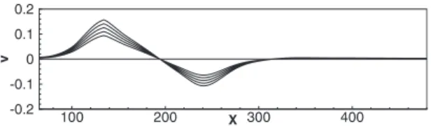
veloc-ity vector, whereas at outlet points, a standard convective condition is employed. At the bottom wall, the no-slip boundary condition is prescribed. Finally, at the upper-boundary points, a suction-and-blowing profile for the v-component of the velocity25is imposed共five profiles with different magnitudes have been considered, see Fig.1兲, and

the vorticity is set to zero.

III. NUMERICAL METHODS A. 2D direct numerical simulation

The NS equations are integrated by a fractional step method using a staggered grid.22The viscous terms are dis-cretized in time using an implicit Crank–Nicholson scheme, whereas an explicit third-order-accurate Runge–Kutta scheme is employed for the nonlinear terms. A second-order-accurate centered space discretization has been used for the linear terms, whereas for the present calculations, a sixth-order-accurate space discretization has been implemented for the nonlinear terms based on a combined compact scheme for nonuniform grids.23The basic idea of such a method is to relate the values of the unknown and of its first and second derivatives at three neighboring grid points. Moreover, since the NS equations are integrated on a staggered grid, a three-point sixth-order-accurate interpolation formula has also been employed to compute the values of the unknowns at the cell centers.

All numerical simulations provided in the present work have been performed discretizing the computational domain by a 501⫻150 Cartesian grid stretched in the wall-normal direction, the height of the first cell close to the wall being equal to 0.1. The Appendix provides a numerical grid-convergence study.

B. Newton procedure for the base flow

The above DNS method has been used to perform all the nonlinear simulations and to compute the base flow for the global stability analysis at subcritical Reynolds number. However, using the DNS, the residual cannot be reduced to machine zero when computing the base flow at supercritical as well as at slightly subcritical Reynolds numbers since some frequencies present in the numerical noise are ampli-fied. In these cases, several approaches may be employed to compute the base flow based on filtering techniques26or on continuation methods. Here, a time-stepping continuation method has been employed. Therefore, following the proce-dure proposed in Ref. 24, the DNS method has been com-bined with a Newton steady-state solver. The steady-state NS equations are written as

X v 100 200 300 400 -0.2 -0.1 0 0.1 0.2

FIG. 1. Suction-and-blowing profiles imposed at the upper boundary for the

N共q兲 + L共q兲 = 0, 共2兲 where q =共u,p兲 and

L共q兲 = 1 Reⵜ

2_{u, N共q兲 = − 共u · ⵜ兲u − ⵜp 共3兲} are the linear and nonlinear operators, respectively. In order to find the solution of Eq. 共2兲, Newton’s method is used. Starting from an initial solution q0, the variable q is itera-tively updated by means of an increment ␦q, computed by

solving the following equation:

共Nq+ L兲共␦q兲 = 共N + L兲共q兲, 共4兲

where Nq is the linearized operator N. By choosing the

op-erator ⌬t共I−⌬tL/2兲−1 _{as a preconditioner of Eq. 共4兲, one} obtains the following equation:

冋

冉

I −⌬tL 2

冊

−1

冉

I +⌬tNq+ ⌬tL 2

冊

− I

册

共␦q兲 =

冋

冉

I −⌬tL 2

冊

−1

冉

I +⌬tN + ⌬tL 2

冊

− I

册

共q兲. 共5兲 It is noteworthy that the solution of Eq.共5兲can be iteratively computed using the existing DNS algorithm with minor modifications since the fractional step operator, obtained by considering the implicit time discretization of the term L共q兲, and the explicit discretization of N共q兲,

qn+1₌

冉

_{I −}⌬tL 2

冊

−1

冋

I +⌬tN +⌬tL 2

册

q n_{, 共6兲}

have been formally recovered. The Newton method has been used for the computation of the base flows at super-critical Reynolds numbers and at slightly subsuper-critical ones 共Reⱖ207兲. In the subcritical case, the residual has been re-duced to 10−12 _{in three up to ten Newton’s iterations,} whereas in the supercritical case, the iterations have been stopped when a residual level of 10−10_{has been achieved due} to a slower convergence of the algorithm.

C. Global eigenvalue analysis

Once the base flows have been computed for several values of the Reynolds number, their global stability is stud-ied by means of a perturbative technique, namely, by consid-ering the instantaneous variable q as a superposition of the base flow and of the perturbation q

⬘

=共u

⬘

,v

⬘

, p

⬘

兲T_{. Such a}

perturbation is decomposed in temporal modes as

q

⬘

共x,y,t兲 =

兺

k=1 N_t

␬k0qˆk共x,y兲exp共− i␻kt兲, 共7兲

where Ntis the total number of modes, qˆkare the

eigenvec-tors, ␻k are the eigenmodes 共complex frequencies兲, and ␬k

0 represents the initial energy of each mode. A substitution of such a decomposition in Eq.共1兲 and a successive lineariza-tion lead to the following eigenvalue problem:

共A − i␻kB兲qˆk= 0, k = 1, . . . ,Nt. 共8兲

The problem 共8兲 is discretized with a Chebyshev/ Chebyshev collocation spectral method employing Nt= 850

modes, and is solved with a shift-and-invert Arnoldi algo-rithm using theARPACKlibrary,27the residual being reduced to 10−12_{. At the upper and inlet boundaries, a zero} perturba-tion condiperturba-tion is imposed, whereas at the outflow, the flow being locally unstable, a Robin condition based on the ap-proximation of the local dispersion relation is prescribed.20,21 Concerning the subcritical flow computations, the modes are discretized using Nx= 250 collocation points in the

x-direction and Ny= 48 collocation points in the y-direction.

The Appendix provides a numerical study for the grid sensi-tivity of the solution. For supercritical flow simulations, a slightly finer grid with Nx= 270 and Ny= 50 has been chosen

due to the reduction in the boundary-layer displacement thickness.

IV. ANALYSIS OF THE RESULTS A. Asymptotically stable dynamics:

Transient growth and convective instabilities

1. Linear dynamics

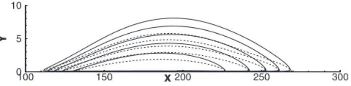
Figure 2shows the streamwise velocity contours of the base flow 1共BF1兲 at Reynolds number Re=200, which has been obtained by imposing at the upper boundary the suction-and-blowing velocity profile with maximum magni-tude shown in Fig.1. BF2, BF3, BF4, and BF5 have been obtained by scaling such a profile by factors 0.9, 0.8, 0.7, and 0.6, respectively. A blowup of the separated zone is provided in Fig.3for all of the base flows, showing the decrease in the bubble size for decreasing values of thev velocity imposed at the upper boundary. For such base flows, the global eigen-value analysis has been performed. Figure4shows the spec-tra for BF1, BF3, and BF5. All the specspec-tra are found to be stable, although it can be noticed that for an increasing bubble size the eigenmodes rise up toward the␻i= 0 axis. By

inspecting the spectra, three families of modes can be de-tected, two of them having a very low growth rate. The asymptotic behavior of the flows is driven by the most

un-x y 100 200 300 400 0 5 10 15 20 25 0.9 0.75 0.6 0.45 0.3 0.15 0 -0.15 x y 100 200 300 400 0 5 10 15 20 25

FIG. 2.共Color online兲 Streamwise velocity contours of the BF1 at Reynolds number Re= 200. The black line is the separation streamline, whereas the dashed line represents the u = 0 contour.

x Y 100 150 200 250 300 0 5 10

FIG. 3. Separation streamlines共solid lines兲 and streamwise zero-velocity contours 共dashed lines兲 of BF1, BF2, BF3, BF4, and BF5 共from top to bottom兲 at Reynolds number Re=200.

stable modes, labeled␻1and␻2in Fig.4for BF1, located on the upper branch of the spectrum. Looking at the eigenvec-tors corresponding to such modes, shown in Figs.5共a兲and

5共b兲, one can observe that they are reminiscent of the classi-cal Tollmien–Schlichting 共TS兲 modes predicted by a local approach.1 This is in agreement with previous results ob-tained by a global analysis for an attached laminar boundary-layer flow19–21and for a cavity-induced separated boundary-layer flow.28However, although the modes have been found asymptotically stable, they are likely to interact leading to a transient amplification of the perturbations due to the nonor-thogonality of the corresponding eigenvectors. With the aim of measuring such an amplification, let us define the energy of the perturbations at time t as

E共t兲 = 1 2

冕

₀ L_x

冕

0 L_y 共u

⬘

2_+v

_⬘

2_{兲dxdy. 共9兲} Furthermore, the maximum energy gain G共t兲, obtainable at time t over all possible initial conditions, u₀

⬘

, is defined as

G共t兲 = max

u₀⬘⫽0

E共t兲

E共0兲. 共10兲

By decomposing the perturbation into the eigenmode basis

共7兲, it is possible to rewrite Eq.共10兲in the following form:

G共t兲 = 储F exp共− it⌳兲F−1储22, 共11兲 where ⌳ is the diagonal matrix of the eigenvalues, ␻k,

and F is the Cholesky factor of the energy matrix, M, of components,

Mij=

冕冕

共uˆiⴱuˆj+vˆiⴱvˆj兲dxdy, i, j = 1, ... ,N, 共12兲

where the superscript ⴱ denotes the complex conjugate. Fi-nally, the maximum amplification at time t and the corre-sponding optimal initial condition, u₀

⬘

, are computed by a singular value decomposition of the matrix F exp共−it⌳兲F−1_.1 Figure 6 provides the maximum energy gain G共t兲

ob-tained for BF1, BF2, BF3, BF4, and BF5 by choosing N = 600 modes among the Nt total modes employed for the

global eigenvalue analysis. A numerical study of the sensi-tivity of the optimal energy gain curve with respect to the number of modes N is provided in the Appendix. The energy gain curves for the five base flows here considered show a similar shape, although the maximum value of the energy gain, G_max, as well as the time at which such a value is achieved, increases with the bubble size. Figure7 provides the variation in G_max with respect to three features of the base flows, namely, the maximum value of the suction veloc-ity at the upper boundary, v_max; the maximum value of the shape factor, H =␦ⴱ/⌰ 共where ⌰ is the momentum thickness of the boundary layer兲; and the aspect ratio of the bubble, which is defined as the ratio between the maximum height of the separated region, h 共measured at the zero-streamwise-velocity line兲, and the length of the bubble. Figure7shows an approximatively linear increase in the Gmaxwith respect to all of the three parameters. It is noteworthy that the aspect ratio of the smallest bubble is close to the ones experimen-tally measured for laminar separation bubbles on the suction surface of aerofoils at a large angle of attack,29,30whereas the largest bubble has a shape factor which is comparable to the one analyzed in Refs.3 and31.

The dashed line in Fig.8shows the linear transient time evolution of the energy gain, E共t兲/E共0兲, obtained by the glo-bal eigenvalue analysis using the initial perturbation, u₀

⬘

max, which provides the maximum peak value at Re= 200 for

ω ω 0 0.05 0.1 0.15 -0.04 -0.03 -0.02 -0.01 0 _{ω ω} 1 2 r i

FIG. 4. 共Color online兲 Eigenvalue spectrum for BF1 共diamonds兲, BF3 共squares兲, and BF5 共circles兲 at Re=200. The modes labeled␻1and␻2are

the most unstable ones.

x y 100 200 300 400 0 5 10 15 20 25 (a) x y 100 200 300 400 0 5 10 15 20 25 (b)

FIG. 5. Streamwise velocity components of the eigenvectors corresponding to the eigenvalues labeled共a兲␻₁and共b兲␻₂in Fig.4. Solid-line contours indicate positive velocities; dashed-line ones are associated with negative velocities. t G (t ) 0 200 400 600 800 1000 100 102 104 106 108 1010

FIG. 6. Optimal energy gain curves at Re= 200 computed by the global eigenvalue analysis for BF1共solid line兲, BF2 共dashed line兲, BF3 共dashed-dotted line兲, BF4 共long-dashed line兲, and BF5 共dashed-dotted-dotted line兲.

BF1. Such a curve is almost coincident with the G共t兲 one, shown by the solid line in Fig. 8 for the same number of modes, N = 600. Both curves reach a maximum value of or-der of magnitude 109_{at t = 410, meaning that the linearized} operator related to the considered flow has a high degree of non-normality.

In order to get some insight into the amplification mechanism, the evolution of such an optimal perturbation in time is analyzed. Figure 9共a兲 shows that at time t = 0 the energy of the optimal perturbation is concentrated in the up-stream part of the bubble. At t = 200关Fig.9共b兲兴, the distur-bance has been convected downstream by the base flow along the separation streamline through a KH mechanism, and it has been amplified before reaching the reattachment point. Such an amplification is due to the local convective instability of the velocity profiles within the bubble, which leads to a global growth of the perturbations, as theoretically demonstrated in Ref. 32 using the Ginzburg–Landau equa-tion for nonparallel flows. After the reattachment point关Fig.

9共c兲兴, the perturbation is convected through the attached

boundary layer, where it is damped. The same convective mechanism has been recovered for BF2, BF3, BF4, and BF5, explaining the linear increase in Gmax and of the time at which it is reached for an increase in the bubble size. It is worth to notice that the energy gain values recovered by the global eigenvalue analysis are quite high. Nevertheless, one has to consider that these are optimal values, therefore the amplification for a real perturbation could be much lower. It is anticipated that for small bubbles, the amplification of the disturbances could be too low to induce nonlinear effects. For this reason, an investigation will be performed of the amplification of a random white-noise disturbance, forced at the inlet or in the whole domain.

Due to the similarities recovered in the transient behav-ior of the different base flows, the following analysis will be carried out only for the separated flow BF1.

2. Weakly nonlinear dynamics

In order to validate the results of the linear stability analysis and to study the weakly nonlinear behavior of the considered separated flow, the DNS has been performed ini-tializing the simulation by superposing the optimal perturba-tion upon the base flow. In order to satisfy the hypothesis of small perturbations, thus allowing a comparison with the re-sults of the global eigenvalue analysis, the optimal distur-bance, u₀

⬘

max, has been scaled by a factor A₀= 10−8_{, which is} four orders of magnitude greater than the residual noise. The energy of the disturbance defined in Eq.共9兲, normalized by the value at t = 0, has been computed at each time step and is reported in Fig.10using the dashed line. In order to verify that a perturbation of order of magnitude A0= 10−8 is small enough to allow a meaningful comparison with the linear model, a linearized DNS has been performed as well, whose result, shown by the dotted line in Fig.10, has been found identical to the one obtained by the DNS. Indeed, by inject-ing an initial perturbation with order of magnitude 10−8_, which corresponds to an initial energy of order of magnitude 10−16, such a perturbation amplifies itself up to a factor of v G 0.09 0.1 0.11 0.12 0.13 0.14 0.15 0.16 105 106 107 108 109 ma x max (a) H G 2.5 3 3.5 4 4.5 5 5.5 6 105 106 107 108 109 ma x (b) h/L G 0.02 0.024 0.028 0.032 0.036 0.04 105 106 107 108 109 ma x (c)

FIG. 7. Maximum value of the optimal energy gain computed by the global eigenvalue analysis at Re= 200 vs共a兲 the maximum suction velocity at the upper boundary,共b兲 the shape factor, and 共c兲 the aspect ratio for BF1, BF2, BF3, BF4, and BF5共from right to left兲.

t E (t )/ E (0 ) 0 200 400 600 800 1000 100 102 104 106 108 1010

FIG. 8. Optimal energy gain curve共solid line兲 and evolution of the normal-ized energy corresponding to the initial perturbation giving the optimal en-ergy peak共dashed line兲 at Re=200, both computed by the global eigenvalue analysis for BF1. x y 100 200 300 400 0 5 10 15 20 25 (a) x y 100 200 300 400 0 5 10 15 20 25 (b) x y 100 200 300 400 0 5 10 15 20 25 (c)

FIG. 9. Streamwise velocity contours of the optimal perturbation obtained by the global eigenvalue analysis for BF1 at time共a兲 t=0, 共b兲 t=200, and 共c兲

t = 400. Solid-line contours indicate positive velocities; dashed-line ones are

109_{, reaching an energy level about equal to 10}−7_{, which is} low enough for nonlinear effects to be negligible. Moreover, Fig. 10 shows that the optimal perturbation energy growth curve obtained with the global eigenvalue analysis, provided by the solid line, is very close to the one computed by the DNS 共dashed line兲, validating the capability of the global model to predict the linear transient mechanism.

However, although the DNS has confirmed the convec-tive amplifier character of the considered separated flow for an optimal initial perturbation, there is no evidence that such a flow would behave similarly in a real case. For this reason, simulations have been performed in which the base flow is perturbed using a time-varying pseudorandom zero-mean Gaussian white-noise disturbance. The flow has been per-turbed in two different ways. In the first case共A兲, a distur-bance field is impulsively injected in the whole domain. In the second case共B兲, the perturbation is superposed upon the inlet velocity profile, as it may happen in real experiments, where the inlet flow may be affected by some noise. In both cases a strong energy gain has been observed, which is ap-proximatively two orders of magnitude lower than the opti-mal one. As shown in Fig.11, the shape of the amplification curves is not far from the optimal one, although some differ-ences can be noticed. In particular, the algebraic growth phase is delayed with respect to the optimal case. This is due

to the fact that the perturbation is damped until it is con-vected by the base flow along the separation streamline, where it begins to be amplified. Due to such an initial delay, the time instant at which the amplification peak occurs 共tmax_A= 460, for case A, and at tmax_B= 490, for case B兲 is greater with respect to the optimal case. It is noteworthy that for case B, in which the inflow perturbation is continuously injected into the flow, the normalized energy does not decay for t⬍150 and t⬎1100, but assumes a value slightly greater than 1. Indeed, for t⬎1100, after the first wave packet has been advected through the separated zone, a statistically steady state is established, so that the continuously injected perturbations do not experience more transient amplification. Nevertheless, some highly sensitive frequencies are excited by the random forcing at the inlet,33and are slightly ampli-fied also after the transient has passed, so that the energy gain maintains asymptotically a value close to 1. Therefore, it is possible to conclude that even though the base flow is continuously perturbed, its response to a small amplitude perturbation is comparable to the response to an impulsive perturbation, which could mean that the strong transient am-plification of the perturbations is a robust feature of sepa-rated flows. Such results are in agreement with previous ones obtained for a flow over a backward facing step perturbed by an inflow random disturbance.6,33

Finally, in order to understand the role of the separated region on such a dynamics, several DNSs have been per-formed in which the perturbation is respectively placed up-stream 共70⬍x⬍100兲, downstream 共280⬍x⬍340兲, and within the bubble in its first half 共120⬍x⬍180兲 or in its second half共200⬍x⬍260兲. Figure12 shows that a pertur-bation placed upstream or within the bubble is amplified, whereas a disturbance initially located downstream of the bubble is damped. In particular, the dynamics of a perturba-tion placed in the first half of the bubble is comparable to the dynamics of case A, whereas a perturbation placed in the second half of the bubble is only weakly amplified, confirm-ing that the amplification mechanism is based on the convec-tion of perturbaconvec-tions along the separaconvec-tion streamline.

t E (t )/ E (0 ) 0 200 400 600 800 1000 100 102 104 106 108 1010

FIG. 10. Time evolution of the energy gain of the optimal initial perturba-tion obtained by the global eigenvalue analysis共solid line兲, by the DNS 共dashed line兲, and by the linearized DNS 共dotted line兲.

t E( t) /E (0 ) 0 500 1000 10-4 10-2 100 102 104 106 108 1010

FIG. 11. Time evolution of the energy gain computed by the DNS for an optimal initial perturbation共solid line兲, for a disturbance field injected in the whole domain共case A, dashed line兲, and for a time-varying disturbance superposed upon the inlet velocity profile共case B, dashed-dotted line兲.

t E (t )/ E (0 ) 0 500 1000 1500 10-5 10-3 10-1 101 103 105 107 109

FIG. 12. Time evolution of the energy gain computed by the DNS for an initial perturbation placed upstream共solid line兲, downstream 共dashed-dotted line兲, or within the bubble in its first half 共short-dashed line兲 or in its second half共long-dashed line兲.

3. Nonlinear dynamics and sensitivity response

In order to study the role of nonlinear effects in the dynamics of a separated flow, nonlinear simulations have been performed increasing the amplitude of the initial pertur-bation, u₀

⬘

max. Figure13provides the energy gain curves ob-tained scaling the optimal perturbation by a factor A₀equal to 10−8_{, 10}−6_{, 10}−5_{, and 10}−4_{, respectively. All of the curves} initially follow the algebraic growth phase, but, for ampli-tudes greater than 10−6_{they show a reduced peak value with} respect to the linear case. For A₀= 10−4_{, a saturation plateau} starts immediately after the initial algebraic growth phase around a value about equal to 107_{. For all cases, the} pertur-bations eventually decay. It is worth to notice that for

A₀ⱖ10−6_{, the decaying rate is lower than the linear one due} to the capability of the nonlinear terms to transfer the energy back in the upstream part of the bubble. It is possible to visualize such a mechanism by inspecting, at a fixed wall normal position, the evolution in time of the perturbation that propagates along the streamwise direction. Indeed, compar-ing the evolution of the linear and nonlinear wave packets shown in Fig.14, one can see that in the second case 关Fig.

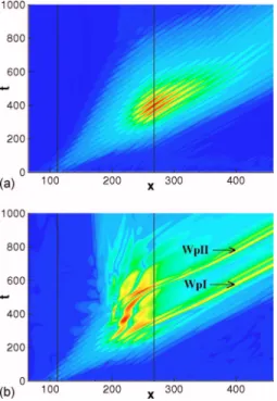
14共b兲兴, a part of the perturbation is driven back in the sepa-rated region, where it interacts with the main part of the wave packet 共WpI兲 which is being convected downstream. As a result, a second wave packet 共WpII兲 appears in the bubble, which is convected in the attached-flow region. Looking at Fig.15, which shows the evolution in time of the vorticity perturbation,␻z

⬘

, at wall at a fixed streamwise

po-sition共x=400兲, it is possible to notice that the amplitude of the two wave packets convected downstream is comparable, meaning that a wave packet cycle starts to be established within the bubble, but it is eventually damped.

In order to study the development of the wave packet downstream of the bubble, a longer computational domain has been considered, Lx

⬘

= 5Lx. As shown in Fig. 16, for

A0= 10−4 and 1000⬍t⬍4000, the perturbation is amplified, whereas for A0= 10−8 and t⬎1000, it is damped when the same domain length is used. Looking at the evolution of the wave packet in time, provided in Fig. 17, it is possible to notice that the perturbation is amplified while it is convected

t E (t )/ E (0 ) 0 500 1000 1500 2000 100 102 104 106 108 1010

FIG. 13. Time evolution of the energy gain computed by the DNS for an optimal initial perturbation with order of magnitude A0= 10−4共solid line兲,

A0= 10−5 共short-dashed line兲, A0= 10−6 共long-dashed line兲, and A0= 10−8

共dashed-dotted line兲.

FIG. 14.共Color online兲 Space-time diagram of the vorticity perturbation at wall,␻z⬘, computed by DNS for an optimal initial perturbation normalized

by factors共a兲 A₀= 10−8_{and共b兲 A}

0= 10−4. The black lines indicate the

sepa-ration and reattachment points of the base flow, whereas the arrows point at the two wave packets shed by the bubble共WpI and WpII兲.

t ω 500 1000 1500 0 0.1 0.2 z WpI WpII

FIG. 15. Time evolution of the vorticity perturbation at wall computed by DNS for an optimal initial perturbation with order of magnitude A0= 10−4at

the streamwise location x = 400.

t E (t )/ E (0 ) 0 2000 4000 6000 100 102 104 106 108 1010

FIG. 16. Time evolution of the energy gain computed by the DNS for an initial optimal perturbation with order of magnitude A0= 10−4with domain

lengths L = Lx共dashed-dotted line兲 and L=5Lx共solid line兲, and for an initial

optimal perturbation with order of magnitude A0= 10−8and domain length

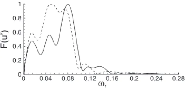
through the attached-flow region, causing a further transient global growth of the energy until it leaves the domain. Such a result indicates that the flow downstream of the bubble is convectively nonlinearly unstable although linearly globally stable. In order to understand the mechanism inducing such an amplification, the Fourier transform in time of the streamwise-velocity fluctuation at two different abscissas, x = 380 and x = 455, has been computed. Figure18shows that immediately downstream of the bubble, the leading mode corresponds to the less stable eigenvalue of the global spec-trum, labeled␻1in Fig.4, whose real part is␻r⬇0.08. Thus,

at such a location the behavior of the flow is driven by the global dynamics. However, for increasing abscissas, the dy-namics is driven by a different mode whose real part is close to␻r⬇0.045. A local spatial stability analysis, which solves

the Orr–Sommerfeld and Squire eigenvalue problem with re-spect to a streamwise wave number␣, has been performed on the velocity base flow profiles at the above streamwise locations. This analysis indicates that such a mode lies in the range of the local spatially unstable frequencies for x = 455, as shown in Fig. 19. The same analysis has been performed at several streamwise locations downstream of the bubble confirming such a result. Thus, one can infer that the wave packet is spatially amplified while it is convected downstream as a consequence of the excitation of a locally unstable mode. In order to find the “critical perturbation” triggering such a mode, several simulations have been per-formed with increasing initial perturbation amplitudes. The streamwise velocity perturbations have been extracted as

they have passed beyond the location x = 455 at two time instants, t = 900 and t = 1000. As shown in Fig. 20, a spatial amplification begins to be noticed for amplitudes equal to 10−6. Such a strong influence of the perturbation amplitude on the behavior of the flow could be due to a high sensitivity to real forcing. Indeed, although the flow is not directly forced with a specific mode, several frequencies are present in the perturbed flow due to the initial impulsive forcing, which could eventually be damped or not depending on the sensitivity of the flow.

The sensitivity of the flow has been studied by adding a forcing term, qˆfe−i␴t, to the linear evolution equation共8兲,␴

being a real frequency.34The solution of the problem is

qˆ = qˆ0eDt− qˆfe−i␴t/共i␴B − A兲, 共13兲

where qˆ0is the initial condition and D is the diagonal matrix, Dk,l= −i␦k,l␻k. Since the flow is globally stable, the solution

for long times is governed by the term −qˆfe−i␴t/共i␴B − A兲.

Moreover, since the influence of an external real harmonic forcing is determined for long times by qˆf, it is possible to

compute the sensitivity to a real external frequency through the analysis of the norm储共i␴B − A兲−1储.34Such an analysis is performed through the evaluation of the pseudospectrum of the global linear operator defined as

␭␧=兵␴苸 C,储共i␴B − A兲−1储 ⱖ ␧−1其. 共14兲 Figure 21provides the pseudospectrum of the flow consid-ered here, represented plotting the contours of −log10共␧兲. At each point on the real axis共␻i= 0兲, the contour value

repre-sents the sensitivity of the flow to external forcing with the corresponding pulsation␻r. The response to a real frequency

X Y 200 400 600 800 1000 0 10 20 (a) X Y 200 400 600 800 1000 0 10 20 (b) X Y 200 400 600 800 1000 0 10 20 (c)

FIG. 17. Contours of the streamwise velocity perturbation, u⬘, computed by the DNS at three time instants:共a兲 t=2200, 共b兲 t=2600, and 共c兲 t=3000. The line on the left indicates the separation streamline.

ω F (u’) 0 0.04 0.08 0.12 0.16 0.2 0.24 0.28 0 0.2 0.4 0.6 0.8 1 r

FIG. 18. Fourier spectrum in time of the streamwise velocity perturbation at the first grid point in the wall normal direction computed by the DNS for two streamwise locations: x = 380共solid line兲 and x=455 共dashed line兲.

ω α 0.02 0.04 0.06 0.08 -0.02 -0.015 -0.01 -0.005 0 r i

-FIG. 19. Spatial amplification rate, −␣i, vs the real pulsation,␻r, computed

by local eigenvalue analysis at two streamwise locations: x = 380共solid line兲 and x = 455共dashed line兲.

FIG. 20. Evolution in the streamwise direction of the streamwise perturba-tion velocity, u⬘, computed by the DNS at a fixed wall normal position,

y = 1.49, for two time values, t = 900共dashed line兲 and t=1000 共solid line兲,

for initial perturbations scaled by factors 共a兲 A0= 10−7 and 共b兲 A0= 10−6,

is dominated by the global KH/TS-like modes, the most sen-sitive one corresponding to the most unstable one.15 Con-cerning the locally unstable mode with␻r⬇0.045, it lies in

the range of the highly sensitive modes. As shown in Fig.21, the minimal perturbation amplitude triggering the real fre-quencies around␻r⬇0.045 is approximatively 10−6, which

matches the value previously found by DNS共see Fig.20兲.

Finally, in order to investigate if such a mechanism link-ing sensitivity and convective instability may be found also in other flow configurations, several DNSs with increasing Reynolds number have been performed. At Re= 223, an as-ymptotically unstable dynamics is recovered by superposing upon the base flow a perturbation of order of magnitude A0= 10−4, while asymptotic stability is obtained with a smaller perturbation. As shown in Fig. 22, the normalized energy saturates at a value of 109, which is maintained as-ymptotically, leading to a periodic self-sustained state. Since the period of the oscillations is about T⬇110, it is possible to identify the locally unstable pulsation,␻⬇0.055, which is very close to the one previously found for Re= 200. There-fore, it is likely that the generation of such a self-sustained state is due to the high sensitivity of the flow to that locally unstable frequency which leads the flow to a subcritical tran-sition. Such results show that the convective modes are a relevant feature of a separated boundary layer flow, being able to arise from different mechanisms 共such as non-normality and sensitivity兲 in both a linear and a nonlinear framework, and are able to play an active role in subcritical transition.

B. Asymptotically unstable dynamics: The origin of unsteadiness and the flapping frequency

1. Linear dynamics

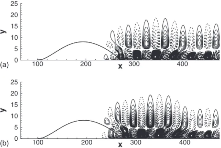
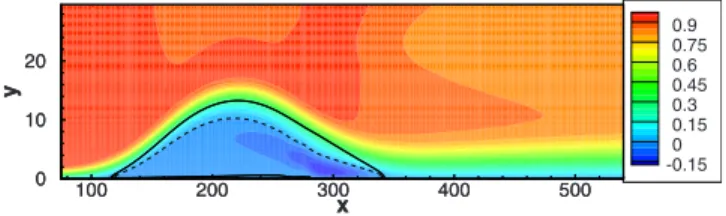
The supercritical dynamics of the flow has been investi-gated by performing the global eigenvalue analysis with in-creasing Reynolds numbers. Transition has been found to occur at Re= 225; Fig.23 shows the corresponding stream-wise velocity contours of the base flow. The structure of the spectrum at such a Reynolds number, provided in Fig.24, is quite similar to the one at Re= 200. The spectrum is margin-ally unstable, since there are seven slightly unstable modes placed on the convective branch, their eigenvectors being reminiscent of the TS waves. Comparing Fig.23with Fig.2, it is possible to notice that for increasing Reynolds numbers, not only the bubble size共defined as the length of the sepa-ration region at the wall兲 increases, but some topological changes occur in the base flow. Looking at the separation streamline, one can observe a smoother reattachment and, most importantly, the presence of a secondary separation zone within the primary one, which is identified by a change in sign of the skin friction coefficient within the primary bubble. Such observations support the hypothesis12,35that to-pological changes in the base flow could be at the origin of the onset of the unsteadiness in separation bubbles. As sug-gested in Ref. 10, it is likely that the primary instability of the considered bubble would be of structural type, meaning that for a supercritical Reynolds number the flow cannot ex-hibit any single-bubble state, instead it is characterized by a multiple separation which induces the vortex formation and shedding, leading to asymptotical instability.

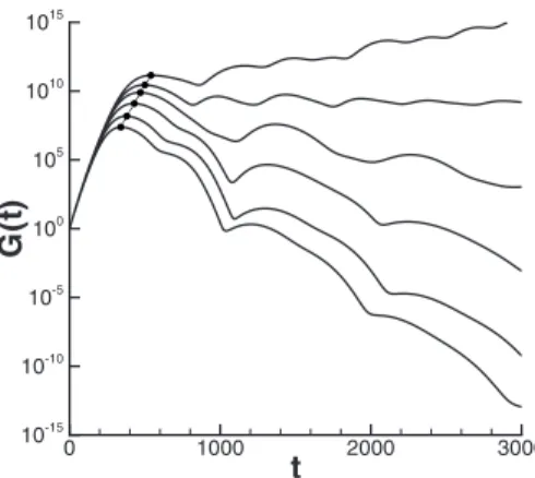
The linear energy growth has been studied using the glo-bal eigenvalue analysis for increasing Reynolds numbers. The behavior of the corresponding energy-gain curves, re-ported in Fig.25, shows that共i兲 the first peak value increases linearly with respect to Re, and共ii兲 the time at which the first

3.5 4.5 5.5 6.5 6.5 _6.5 7.5 7.5 8.5 8.5 ω ω 0 0.04 0.08 0.12 0.16 0.2 -0.03 -0.02 -0.01 0 9.5 8.5 7.5 6.5 5.5 4.5 3.5 2.5 i r

FIG. 21. 共Color online兲 Pseudospectrum contours represented using the logarithmic scale −log10共␧兲. The vertical solid line indicates the most

sensi-tive pulsation共␻r⬇0.085兲, whereas the vertical dashed line indicates the

sensitivity value to a forcing of pulsation␻r⬇0.045.

t E (t )/ E (0 ) 0 2000 4000 6000 100 102 104 106 108 1010

FIG. 22. Time evolution of the energy gain computed by the DNS for an initial optimal perturbation of order of magnitude A0= 10−4at Re= 223.

x y 100 200 300 400 500 0 10 20 0.9 0.75 0.6 0.45 0.3 0.15 0 -0.15 x y 100 200 300 400 500 0 10 20

FIG. 23. 共Color online兲 Streamwise velocity contours of the base flow at Reynolds number Re= 225. The solid line is the separation streamline, whereas the dashed line represents the u = 0 contour.

ω ω 0 0.05 0.1 0.15 -0.03 -0.02 -0.01 0 ω ω ω1 3 2 i r

FIG. 24. 共Color online兲 Eigenvalue spectrum for the flow at Re=225 with

Nx= 270 and Ny= 50 grid points. The modes labeled␻1,␻2, and␻3are the

peak occurs increases linearly with respect to Re. Recalling that the transient energy growth in the considered case is due to the KH amplification along the separation streamline, one can assume that the increase in G共t兲 is due to the increase in the size of the bubble with the Reynolds number. Indeed, plotting the bubble size versus the Reynolds number, a linear dependence is recovered, as shown in Fig.26.

In the slightly unstable case 共Re=225兲, a linear energy gain equal about to 1012_{has been found, as shown by the top} curve in Fig. 25, which is a very high amplification with respect to the data available in the literature for other flow configurations. For instance, in Ref. 8, for a separated flow over a bump the authors found a peak value about equal to 109 _{for the critical Reynolds Re}

␦= 590, whereas here

a growth of order of magnitude 1012 _{is observed for} Re_␦= 225. Such a difference is clearly dependent on the bubble size and could also be due to the absence of solid boundaries bordering the bubble, which allows the perturba-tion to amplify itself along the separaperturba-tion streamline from the separation point to the reattachment one.

In order to further investigate the linear unstable dynam-ics of an initial perturbation, the evolution of the optimal perturbation at Re= 225 has been studied. As shown in Fig.

27, the perturbation is initially convected downstream by the mean flow as a localized wave packet. However, unlike the stable case previously analyzed, a second wave packet is generated due to the amplification of the disturbances carried back by the recirculation bubble. Such a disturbance shed-ding cycle is not due to an absolute instability of the velocity profiles within the bubble, as assessed by a local eigenvalue analysis, but to the global characteristics of the flow. It is

worth to notice that the subcritical transient growth mecha-nism in a nonlinear framework analyzed in Sec. IV A 3 seems to be not far from the asymptotically unstable mecha-nism shown here. In the subcritical case, the nonlinear terms being able to transfer energy among different modes, a wave packet cycle begins to be established until it decays due to the asymptotical damping of the perturbation. Thus, the gen-eration of wave packets by the cyclic transfer of energy from the upstream part to the downstream part of the bubble and vice versa seems to be a feature of the stability dynamics of such a separated flow.

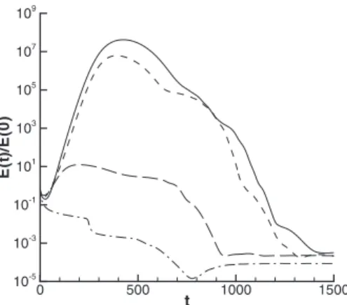
Focusing now on the asymptotic behavior of the flow at different Reynolds numbers, one can observe in Fig.25that each energy gain curve is affected by a modulation. Such a modulation, also named beating or flapping frequency, is a well-known feature of separated flows,8,28 although it has been found for the first time in a falling curtain flow.18Such a phenomenon is due to the interaction of the most unstable modes of the spectrum. In Fig.4共Re=200兲, one can observe

two modes, labeled␻₁ and ␻₂, having comparable amplifi-cation rate. Since such modes are associated with similar eigenvectors, they are able to interact resulting in the low frequency modulation observed for the energy gain curve at Re= 200. In fact, since the real parts of these eigenmodes differ at about␦␻r= 0.006, their interaction results in a wave

packet of period T = 2␲/␦␻r⬇1000, which corresponds to

the modulation shown in Fig.28by the energy gain curve for Re= 200 共dashed line兲. Moreover, it appears from Fig. 25

that two frequencies can be identified for each energy gain curve with Reⱖ213. For instance, at Re=225, the first fre-quency共labeled as I兲 corresponds to the low-frequency beat-ing found in the previous case, havbeat-ing a period of about T⬇850 共see the solid line in Fig.28兲. The second frequency

t G( t) 0 1000 2000 3000 10-15 10-10 10-5 100 105 1010 1015

FIG. 25. Optimal energy gain curves obtained by the global eigenvalue analysis with N = 400 modes for increasing Reynolds numbers: from the bottom curve to the top one, Re= 190, 200, 207, 213, 219, and 225, respectively. Re L 150 160 170 180 190 200 210 220 230 0 5 10 15 20 25 30 b δ ∗

FIG. 26. Dimensional bubble size Lb␦ⴱvs Re.

(b) x y 100 200 300 400 500 0 10 20 30 (a) (c) (d) (e)

FIG. 27. Snapshots of the streamwise perturbation velocity contours for the optimal perturbation obtained by the global eigenvalue analysis for Re = 225 at共a兲 t=0, 共b兲 t=450, 共c兲 t=650, 共d兲 t=850, and 共e兲 t=1050. Solid-line contours indicate positive velocities; dashed-Solid-line ones are associated with negative velocities.

共labeled as II兲 is slightly higher than the first one, having a period of about T⬇300. Indeed, by looking at the spectrum at Re= 225, provided in Fig. 24, one can notice that the three most unstable modes have very similar amplification rate, leading to cancellation as in the stable case. Since their real parts differ at about␦␻r_I=␻r₃−␻r₁⬇0.0075

and ␦␻r_II=␻r₂−␻r₃⬇0.02, they result, respectively,

in two wave packets of period T_I= 2␲/␦␻r_I⬇850 and

TII= 2␲/␦␻r_II⬇300. It is worth to notice that due to the

lin-earity of the global eigenvalue analysis, for large values of t the beating induced by the two most unstable modes 共fre-quency II兲 dominates the other one, as reported in Fig.28. The sensitivity of such results with respect to the grid reso-lution and the domain length is discussed in the Appendix.

2. Nonlinear dynamics

The physical mechanism governing the beating phenom-enon has been studied by performing several numerical simulations with increasing Reynolds numbers. DNS pre-dicts transition at Re= 230, which is close but not exactly equal to the critical Reynolds number obtained by the linear analysis, namely, Re= 225. Such a discrepancy might be due to a stabilizing effect of the convective outflow boundary conditions, as conjectured in Ref.8, or to an imperfect con-vergence of the convective branch of the eigenvalue spec-trum, which is very sensitive to numerical parameters, or to the different numerical discretizations used in the global ei-genvalue analysis and DNS. Superposing the optimal pertur-bation obtained by the transient growth analysis upon the base flow at Re= 225, the time evolution of the energy gain has been computed by DNS. In Fig. 29 it is possible to observe that two modulations affect the energy gain curve after the transient has passed, with periods TI⬇1200 and TII⬇350. Such results are in good agreement with the ones found by using the global eigenvalue analysis.

It is worth to notice that the linear peak value of the energy gain 1012_{共see Fig.28兲 is not reached in the nonlinear} case shown in Fig.29, the predicted optimal growth being so high that the energy saturates before. In the considered case,

by injecting an initial perturbation with order of magnitude 10−6_{, which corresponds to an initial energy of order of} mag-nitude 10−12_{, such a perturbation amplifies itself up to a} factor of 1011_{, reaching amplitudes about equal to 10}−1_, so that the nonlinear effects are not negligible. However, as the amplitudes of the perturbations begin to decrease due to asymptotic stability, a linear dynamics is eventually recovered.

At supercritical Reynolds numbers, saturation occurs earlier due to the interactions of exponentially growing wave packets and it is maintained asymptotically. In order to assess if the two flapping frequencies are a feature of the considered flow also at supercritical conditions, the power spectrum in time of the evolving perturbation u

⬘

at a point within the bubble 共x=339, y=1.4兲 has been computed for Re=230. Figure30shows the power density spectrum obtained by the Welch periodogram/fast Fourier transform method of u

⬘

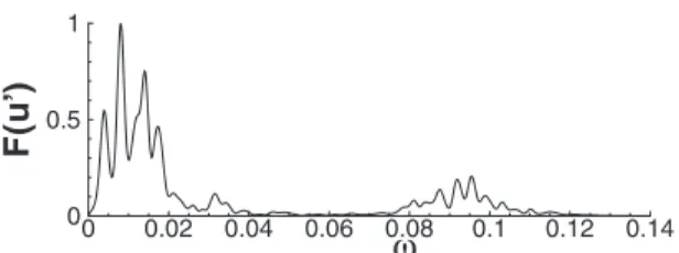
on a sampling period of T = 40 000 divided in eight partially over-lapped windows. A Hamming window function has been used on each data segment. Two frequency ranges where the energy is mostly located are found. The higher frequency range corresponds to TS waves, since the pulsations in the range 0.06⬍␻r⬍0.12 correspond to the globally unstable

modes of Fig.24. Moreover, in the low-frequency region it is possible to recover three leading pulsations which are close to the flapping frequencies I and II and to their difference, respectively 共␻I⬇0.005, ␻II⬇0.014, and ␻III=␻II−␻I ⬇0.009兲.

In order to shed light on the onset of the beating phe-nomenon, the dependence of such modulations on the Rey-nolds number has been investigated. The primary flapping

t

G(

t)

0 1000 2000 3000 4000 10-12 10-7 10-2 103 108 1013 1018 T =850 T =300 I II T =₁₀ 00 I

FIG. 28. Optimal energy gain curves obtained by the global eigenvalue analysis with N = 600 modes for Re= 225共solid line兲 and Re=200 共dashed line兲. t E (t )/ E (0 ) 0 1000 2000 3000 4000 5000 6000 7000 100 102 104 106 108 1010 1012

FIG. 29. Time evolution of the energy gain of an initial optimal perturbation of order of magnitude A0= 10−6computed by the DNS at Re= 225.

ω F( u ’) 0 0.02 0.04 0.06 0.08 0.1 0.12 0.14 0 0.5 1

FIG. 30. Power density spectrum in time of the streamwise perturbation velocity, u_⬘, obtained by a Welch method on a sampling period of T = 40 000 divided in eight partially overlapped windows, for Re= 230 at

frequencies have been computed by means of the global ei-genvalue analysis at several Reynolds numbers lying in the range of 150ⱕReⱕ225. In order to eliminate the depen-dence of the frequencies on␦ⴱ, a Reynolds number based on the reference length L = 0.05 m, ReL= U⬁L/␯ has been

em-ployed, the corresponding dimensionless frequency being F = L/␦ⴱf. Plotting the frequency values versus ReL,

as shown in Fig. 31, it appears that F⬇1 for ReL

ⱕ33 000 共Reⱕ207兲, whereas for ReLⱖ35 000 共Reⱖ213兲,

which is the threshold for the onset of the secondary flapping frequency, the frequency F slightly increases. A possible ex-planation of such a behavior is here provided, which con-cerns the physical mechanism governing the onset of the flapping frequencies in separated flows over a flat plate. Re-calling that the beating is due to the interaction of two modes presenting similar eigenvectors, and that such an interaction has been observed in several separated flows, such as cavity-induced and bump-cavity-induced separations,8,28 it can be argued that a separated region, which is able to carry back the per-turbation, could play an active role in the generation of the interaction between modes. In fact, a part of the perturbation located in the separated region could be convected upstream within the bubble, where it is likely to interact with the main part of the wave packet, which is being convected down-stream along the separation down-streamline. Therefore, one may assume that the beating frequency would be proportional to 1/tL, where tLis the time needed by the mean flow to carry

back such a wave packet from the reattachment point to the separation streamline,

F⬇ 1/tL⬇ Ub/Lb, 共15兲

where Lbis the size of the bubble and Ubthe velocity of the

base flow within the bubble. By measuring the variation in the bubble size and in the velocity at the first grid point from the wall where the maximum backflow is recovered at

dif-ferent Reynolds numbers, it appears that both Lband Ubvary

linearly with respect to ReL when ReL⬍35 000 共Re⬍213,

see Figs.26and32, respectively兲. Such a linear dependence is broken when ReLⱖ35 000 due to some topological

changes in the base flow. Thus, as long as ReL⬍35 000, the

ratio between two frequencies F1 and F2 at two Reynolds numbers ReL₁ and ReL₂could be written as

F₂ F1 ⬇tL1 tL₂ ⬇Ub2 Ub₁ Lb₁ Lb₂ =ReL2 ReL₁ ReL₁ ReL₂ = 1, 共16兲

meaning that the flapping frequency, F, remains constant when the Reynolds number varies, confirming the results shown in Fig.31for ReL⬍35 000.

Concerning the dynamics at ReL= 35 000 共Re=213兲,

looking at the corresponding base flow in Fig.33共a兲, one can see an inflection of the streamlines within the bubble, which is not observed for smaller values of the Reynolds number 关see Fig.33共b兲corresponding to Re= 207兴. The DNS shows that when the flow is perturbed or when the Reynolds num-ber is increased, such a topological change originates a small separation which splits the bubble in two smaller ones, la-beled as part A and part B in Fig.34. It is possible to assume that the onset of the flapping frequency II at such a Reynolds number is a consequence of the splitting of the bubble in two smaller ones, which could carry back the perturbations at two different rates generating two distinct modulations of the energy gain curve. Indeed, one can notice that the ratio of the

Re F 20000 25000 30000 35000 0.5 1 1.5 L

FIG. 31. Values of the dimensionless flapping frequencies, F, vs ReL. The

values of Re at the black square points are 152, 160, 168, 176, 182, 191, 200, 207, 213, 220, and 225, respectively. Re U 20000 25000 30000 35000 -0.15 -0.1 -0.05 ma x L

FIG. 32. Values of the maximum backflow velocity within the bubble vs ReL. The values of Re at the black square points are 152, 160, 168, 176, 182,

191, 200, and 207, respectively, whereas at the empty square points Re= 213, 220, and 225, respectively.

X Y X Y (b) (a)

FIG. 33. Streamlines within the separated region for two base flows at共a兲 Re= 213 and共b兲 Re=207. Within the panel, the inflections of the streamlines for Re= 213 are shown.

x

y

100 200 300 400 0 2 4 6 8 10 12 14 16 Part A Part B

FIG. 34. Streamlines within the separated region for the base flow at Re= 230. The presence of a secondary bubble within the first one divides the bubble in two parts, labeled A and B.

size of bubble A with respect to the size of the bubble B 共LB/LA⬇2.5兲 is very close to the ratio of the two flapping frequencies 共␻II/␻I⬇2.8兲, supporting such an assumption. Moreover, the bubble splitting would also explain why a higher value of the flapping frequency I is recovered for ReLⱖ35 000. Indeed, assuming that the beating I is

gener-ated by the part B of the bubble 共while the beating II is generated by the part A兲, one can argue that such a bubble, which is smaller than the original one, would be able to carry back disturbances in a smaller time, originating a higher pri-mary beating frequency.

In order to validate such a model for the case of smaller bubbles, the onset of the flapping frequency has been inves-tigated for BF2, BF3, BF4, and BF5. Figure35provides the energy gain curves computed by the global eigenvalue analy-sis for BF1, BF2, BF3, BF4, and BF5共from top to bottom兲, showing that a low-frequency modulation is recovered for all of the considered separated flows. The dependence of the flapping frequency, F, on the ratio Ub/Lb has been

investi-gated, where Ub, representing the upstream convection

ve-locity of the base flow, has been measured within the bubble at the first grid point from the wall where the maximum backflow is recovered. Figure36shows that F has approxi-matively a linear variation versus the ratio Ub/Lb, validating

the conjecture of Eq.共15兲. Finally, it should be noticed that the onset of the flapping modulation in the energy gain curve for BF5共see the bottom curve in Fig.35兲 is associated with

very low levels of the normalized energy, about equal to 10−5. Therefore, it is likely that the beating could not be observed in an experimental framework for small size bubbles. Moreover, it has been verified that for a smaller bubble, having an aspect ratio of about h/L⬇0.01, the flap-ping phenomenon is inhibited probably due to the very nar-row shape of the separated zone. For larger bubbles, the flap-ping phenomenon is associated with higher levels of the

energy, in some cases affecting the dynamics of the separated flow also in the presence of nonlinear effects, and becoming observable in experimental measurements.36

V. CONCLUSIONS

The transient and asymptotical dynamics of a large sepa-ration bubble over a flat plate has been studied in order to investigate the role of non-normality and nonlinearity of the differential operator in the stability of such a flow. Two nu-merical tools have been employed, namely, the global eigen-value analysis and the DNS; moreover, a continuation proce-dure based on Newton’s iteration has been used to compute the steady-state solutions of the NS equations at slightly su-percritical Reynolds numbers. Linear eigenvalue analysis, as well as numerical simulations with weakly nonlinear pertur-bations, have shown that the non-normality of convective modes of the NS operator allows the bubble to act as a strong amplifier of small disturbances. In particular, the initial per-turbation allowing the largest energy gain is found to be placed close to the separation point and to be amplified by a Kelvin–Helmholtz mechanism while being convected down-stream. Indeed, the front part of the bubble shows a high sensitivity to external noise, as observed in simulations with white noise disturbances superposed upon the whole base flow or upon the inflow Blasius profile. For finite amplitude initial perturbations, the strong linear transient amplification saturates due to nonlinear interactions between modes. Fur-thermore, such an energy exchange between modes induces the bubble to establish a wave packet cycle, characterized by the shedding of two wave packets of comparable amplitude. Such a cycle is similar to the one occurring at supercritical Reynolds numbers, but it is eventually damped when the t G( t) 0 1000 2000 3000 4000 10-20 10-15 10-10 10-5 100 105 1010

FIG. 35. Energy gain curves computed by the global eigenvalue analysis for BF1, BF2, BF3, BF4, and BF5共from top to bottom兲.

U /L F 0.006 0.008 0.01 0.012 0.014 0.016 0.975 0.98 0.985 0.99 b b

FIG. 36. Value of the flapping frequency F vs the ratio Ub/Lbcomputed by

the global eigenvalue analysis for BF1, BF2, BF3, BF4, and BF5共from right to left兲. t E (t )/ E (0 ) 0 200 400 600 800 1000 100 102 104 106 108 1010

FIG. 37. Energy gain curves obtained by the DNS with a共251⫻75兲 grid 共dashed line兲, a 共501⫻150兲 grid 共solid line兲, and a 共1001⫻300兲 grid 共dashed-dotted line兲. ω ω 0.02 0.04 0.06 0.08 0.1 0.12 0.14 0.16 -0.03 -0.02 -0.01 0 r i

FIG. 38. 共Color online兲 Global spectrum obtained for Re=200 with a 共200⫻40兲 grid 共squares兲 and a 共250⫻48兲 grid 共diamonds兲.

flow is asymptotically stable. Nonlinear interactions contrib-ute also to the excitation of a convectively unstable mode in the attached-flow region due to the high sensitivity of the boundary layer, inducing a further transient amplification of finite amplitude perturbations as well as an asymptotical in-stability at slightly subcritical Reynolds numbers.

Concerning the unstable dynamics of the considered flow, topological flow changes on the base flow have been found to occur close to transition, supporting the hypothesis of some authors12,35 that the unsteadiness of separated flows could be due to structural changes within the bubble. Fur-thermore, non-normality effects have shown to play an active role at large times. In fact, due to the superposition of two convective non-normal modes, a low-frequency oscillation known as flapping frequency appears. Close to transition, when topological changes occur in the flow, a secondary flapping frequency appears as well. A possible explanation of such a behavior has been provided, in which it is assumed that the oscillations are due to the interaction of the main wave packet with the perturbations carried upstream by the backflow inside the bubble. A scaling law based on the pre-vious assumption is able to predict accurately the depen-dence of the flapping frequency on the Reynolds number and the onset of the secondary frequency close to transition. Fu-ture works will focus on the physical description of the flap-ping phenomenon in order to provide a further validation of the above conjecture and to test it in a more realistic three-dimensional case. Preliminary DNS results show that the

flapping frequencies are recovered also in a three-dimensional configuration, and that their values are close to the ones here obtained for the 2D case.

ACKNOWLEDGMENTS

This work was performed using HPC resources from GENCI-CCRT/IDRIS 共Grant 2009-022188兲. The authors would like to thank R. Verzicco for providing the second-order accurate version of the DNS code, F. Alizard for pro-viding the code for the global eigenvalue analysis, and M. Napolitano and A. Lerat for making possible the cooperation between the two laboratories in which this work has been developed. This research has been supported by MIUR and Politecnico di Bari under contracts CofinLab2001 and PRIN2007.

APPENDIX: CONVERGENCE STUDIES

A grid convergence study for the DNS has been formed by computing the energy growth of the optimal per-turbation for the separated flow at Re= 200 using three grids with 251⫻75, 501⫻150, and 1001⫻300 cells, respectively. As shown in Fig. 37, the results obtained using the second and the third grids are very close to each other, so that the 501⫻150 grid, which has been used in all of the computa-tions, can be considered adequate to capture the energy growth of the disturbances accurately.

Concerning the global model, Fig.38shows the spectra obtained for the separated flow at Re= 200 using two grids with 200⫻40 and 250⫻48 collocation points, respectively 共computations with a considerably finer grid are not possible due to memory requirements兲. The shape of the spectra com-puted with the two grids does not show remarkable differ-ences, although the modes are found to slightly change their position. Nevertheless, it is well known that a pointwise con-vergence of the global spectra with respect to grid resolution for highly nonparallel flows cannot be reached due to the high non-normality of the operator,34 see, for instance, the

t G( t) 0 200 400 600 800 1000 100 102 104 106 108 1010

FIG. 39. Optimal energy gain curve at Re= 200 computed with N = 600 modes 共solid line, reference case兲, N=500 modes 共dashed line兲, and

N = 300 modes共dashed-dotted line兲.

ω ω 0 0.05 0.1 0.15 -0.015 -0.01 -0.005 0 0.005 ω ω1 3 ω2 i r

FIG. 40. 共Color online兲 Spectra obtained at Re=225 for three domain lengths: L1= 430共diamonds兲, L2= 480共squares兲, and L3= 530共circles兲.

1 2 3 0 0.01 0.02 0.03 0.04 δω I,II

FIG. 41. Sensibility of the value of the flapping frequencies I 共white squares兲 and II 共black squares兲 to the grid resolution: Nx= 260, Ny= 48共point

1兲; reference case, Nx= 270, Ny= 50共point 2兲; and Nx= 300, Ny= 56共point 3兲.

1 2 3 4 0 0.01 0.02 0.03 0.04 δω I,II

FIG. 42. Sensibility of the value of the flapping frequencies I 共white squares兲 and II 共black squares兲 to the domain length: Nx= 270, Ny= 50,

Lx= 430 共point 1兲; reference case, Nx= 270, Ny= 50, Lx= 480 共point 2兲;