THÈSE
THÈSE
En vue de l'obtention du
DOCTORAT DE L’UNIVERSITÉ DE TOULOUSE
DOCTORAT DE L’UNIVERSITÉ DE TOULOUSE
Délivré par l'Université Toulouse III - Paul Sabatier Discipline ou spécialité : Automatique
JURY
Anibal OLLERO, Professeur École Sup. d'Ingénieurs de Seville, Rapporteur Claude PEGARD, Professeur UPJV Picardie, Rapporteur
Jean-Louis CALVET, Professeur UPS Toulouse, Examinateur Rachid ALAMI, DR CNRS, LAAS, Examinateur
Pascal BRISSET, Professeur ENAC, Examinateur Simon LACROIX, DR CNRS, LAAS, Examinateur
Ecole doctorale : Ecole doctorale Systèmes EDSYS Unité de recherche : LAAS / CNRS
Directeur(s) de Thèse : Simon LACROIX Rapporteurs : Anibal OLLERO, Claude PEGARD
Présentée et soutenue par Panagiotis THEODORAKOPOULOS Le 4 mai 2009
Th`
ese
pr´epar´ee auLaboratoire d’Analyse et d’Architecture des Syst`emes du CNRS
en vue de l’obtention du
Doctorat de l’Universit´e de Toulouse
Sp´ecialit´e : Automatique
par
Panagiotis THEODORAKOPOULOS
On autonomous target tracking for UAVs
Soutenue le 4 mai 2009 devant le jury compos´e de :
Anibal OLLERO Rapporteur
Claude PEGARD Rapporteur
Rachid ALAMI Examinateur
Pascal BRISSET Examinateur
Jean Louis CALVET Examinateur
Simon LACROIX Directeur de th`ese
LAAS-CNRS
7, Avenue du Colonel Roche 31077 Toulouse Cedex 4
Acknowledgements
First of all, I would like to thank the Greek State Scholarship Foundation (I.K.Y.) for offering me the chance to prepare this Ph.D. in France, by financing this project.
Secondly, I would like to express my gratitude to my supervisor, Simon Lacroix, whose great sense of humor, expertise, patience, warm leadership skills, and well-targeted ideas helped me get through this long term project. Simon, thank you a lot, I’ve learned a lot from you and if I started this Ph.D. all over again, I would still do it with you.
Thirdly, I would like to express my gratitude to Raja Chatila and Rachid Alami for accepting me in the robotics group, to Jean-Louis Calvet for participating at the defense jury, to Anibal Ollero and Claude Pegard for reviewing the thesis manuscript and finally to Pascal Brisset for participating in the jury as well as to the whole ENAC team for producing such a useful tool as the Paparazzi autopilot/simulator.
Fourthly, I would also like to thank Bertrand Vandeportaele for his valuable support during the flights, his technical advices and mostly for letting me know what it means to be a real engineer - I hope that you will invite me to see that house of yours when it is completed. A big ’thank you’ to Dimitris Fragkoulis for his support, good times spent around our common washing machine and the laughs we had when we had to drive each other to the airport - I just learned that we could have used one of the airport parking spots instead.
I also would like to thank Gautier Hattenberger for his help not only in the early phases of this thesis but also for his support as a member of the Paparazzi autopilot team, as well as Michel Courdesses for offering some good advises during the early phases of this thesis.
I would like to say a glorious thank you to all the people (and plants) that I’ve spent some time with in room B67. Viviane Cadenat for her jokes and good times, Tereza Vidal for her big smile coming from the other side of the desk, Joan Sola for his engaging ideas, talks and proofreading help, Louis F.Marin for the funny times and proofreading corrections, Norman Juchler for throwing balls of paper at me, eating all my yogurts and organizing cool parties. Finally, I should include in this list, the strange cactus named ’Finis-ta-these’ that kept the atmosphere in the room clean and the spirits high.
A warm thank you to Jerome Manhes, Sara Fleury and the legendary Matthieu Herrb for helping our robots remain functional. I would like to give a special thank you to An-thony Mallet for sharing some talks with me in the Japanese garden as well as answering my programming questions.
Special thank you to: S´ebastien Dalibard and Manish Sreenivasa for their corrections and engaging talks, Mokhtar Gharbi and Xavier Broqu`ere for their help and funny talks, the great Yi Li for every lunch we had together and for helping me get out of the building the days that I left my badge home, Alireza Nakhaei Sarvedani for the laughing moments and Mathieu Poirier for all the drinks and the talks we had together about women. It would be impossible to leave out Sophie Achte, Camille Cazeuneve and Natacha Ouwanssi as they supported me in all my strange administration demands.
I would like to thank more than anything my parents Aristotelis and Katerina Theodor-akopoulos for having worked hard during their lives so that their children can have the chance to think and enjoy an excellent quality of life. To my sister for finishing her studies and mak-ing me jealous so that I had to finish my Ph.D. too, to my grand mother for teachmak-ing me what courage means and to my uncle Thanassis for learning me how to think big.
hennes støtte alle disse ˚arene. Flyturen fortsetter wingman :)
Contents
Glossary 2
1 Introduction 9
1.1 Motivations . . . 9
1.2 Challenges and objectives . . . 10
1.2.1 Problem characteristics . . . 10
1.2.2 Thesis objective . . . 11
1.3 Contributions and Thesis Outline . . . 11
1.3.1 Outline . . . 11
1.3.2 Implementation Grid . . . 12
2 State of the art 14 2.1 Guidance, Navigation and Control . . . 15
2.1.1 Waypoints VS Continuous Navigation . . . 15
2.1.2 Missile Guidance . . . 15
2.1.3 Mixed strategy trajectory following . . . 17
2.1.4 Waypoint Guidance . . . 18
2.1.5 Potential Fields . . . 18
2.1.6 On Non-holonomic Aircrafts and Time Optimal Paths . . . 19
2.1.7 UAV Trajectory Optimization for Target Tracking . . . 20
2.1.8 Synthesis of Guidance, Navigation and Control Bibliography . . . 22
2.2 Planning based methods for UAVs . . . 23
2.2.1 Path Finding for UAVs . . . 23
2.2.2 Search algorithms . . . 24
2.2.3 Variants of Potential Fields . . . 27
2.2.4 Path Finding and Obstacle Avoidance . . . 27
2.2.5 Synthesis of planning methods . . . 28
2.3 Decision: game theory . . . 28
2.4 Competitive Approaches . . . 33
2.5 Cooperative Approaches . . . 39
2.6 Overall Synthesis of State of the Art . . . 41
3 Problem Statement and Formulation 42 3.1 UAV . . . 42
3.1.1 Trajectory . . . 42
3.2 Target . . . 45
3.3 Environment . . . 45
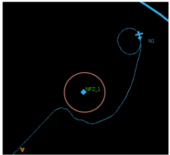
3.3.1 No Fly Zones . . . 45
3.3.2 Visibility Obstructing Obstacles . . . 46
3.3.3 Road Network . . . 46
3.4 Mission criteria . . . 46
3.4.1 Metrics . . . 47
3.5 Synthesis of the problem . . . 48
4 Tracking a target on a ground plane 50 4.1 Problem Statement . . . 50
4.1.1 Overview of our approach . . . 52
4.2 Lateral Guidance . . . 52
4.3 Tracking Strategy . . . 55
4.3.1 Line of sight distance . . . 55
4.3.2 The lateral target image error xf . . . 56
4.3.3 Tracking strategy . . . 56
4.4 Results . . . 57
4.4.1 Simulations . . . 57
4.4.2 Stability assessment for a noisy sensor . . . 59
4.4.3 Flight Tests . . . 61
4.5 Conclusions . . . 63
5 An adversarial iterative predictive approach to target tracking 66 5.1 Problem Statement . . . 66
5.2 Overview of the approach . . . 67
5.3 Evaluation functions . . . 68
5.3.1 UAV Evaluation Function . . . 68
5.3.2 Overall path cost . . . 72
5.4 Prediction and Iterative Optimization . . . 73
5.4.1 UAV prediction . . . 73
5.4.2 Target Prediction . . . 75
5.4.3 Off-road target evaluation function . . . 78
5.5 Results . . . 80
5.5.1 Evaluation of optimization methods . . . 80
5.6 Extension to the multiple UAV target tracking case . . . 83
5.6.1 Two UAV visibility . . . 83
5.6.2 Two UAV strategies . . . 85
5.6.3 Results of the two UAV approach . . . 86
5.7 Conclusions . . . 87
6 A discrete game theoretic approach to target tracking 88 6.1 Introduction . . . 88
6.2 Overview of the Approach . . . 89
6.3 Game space discretization . . . 89
6.4 Analysis . . . 90
6.5 Mono-pursuer decision making . . . 95
6.5.1 Utility Maximization . . . 95
6.5.2 Adversarial Searching . . . 96
6.5.3 Nash equilibria and dominance strategies . . . 97
6.6 Multi-pursuer decision making . . . 97
6.6.1 Hierarchical VS Consensus based approaches . . . 98
6.6.2 Utility Maximization . . . 99
6.6.3 Cooperative Nash equilibria . . . 99
6.6.4 Pareto optimality method . . . 100
6.7 Realization . . . 100
6.8 Extension of the evaluation functions: visibility maps . . . 101
6.8.1 Indicator of Stealthiness . . . 101
6.8.2 Measuring Stealthiness from the air . . . 101
6.9 Results . . . 103
6.9.1 Evaluating the different approaches . . . 103
6.9.2 Mono-pursuer decision making . . . 103
6.9.3 Multi-pursuer decision making . . . 104
6.10 Conclusions . . . 104
7 Conclusions 115 7.1 Summary . . . 115
7.2 Discussion and further work . . . 115
7.2.1 Iterating on the thesis contributions . . . 115
7.2.2 Beyond the horizon of the thesis . . . 117
A Implementation 118 A.1 The Paparazzi Flying System . . . 118
A.1.1 Presentation . . . 118
A.1.2 Hardware . . . 119
A.1.3 Software . . . 121
A.2 Development and Simulation Environments . . . 122
A.2.1 Algorithm encapsulation . . . 122
A.2.2 Scilab simulation platform . . . 125
A.3 Aircrafts-Robots . . . 125
A.3.1 The Nirvana fleet . . . 125
B Resum´e 127 B.1 Motivations . . . 127
B.2 Les d´efis et les objectifs . . . 128
B.2.1 La probl´ematique . . . 128
B.2.2 Les objectives de la th`ese . . . 129
B.3 La contribution et le plan du th`ese . . . 129
B.4 L’´etat de l’art . . . 129
B.5 Synth`ese du probl`eme . . . 130
B.6 Suivre une cible terrestre . . . 131
B.6.1 Vue d’ensemble de notre approche . . . 132
B.7 Une appoche it´erative predictive pour suivre la cible . . . 132
B.8 Fonctions d’´evaluation . . . 134
B.8.1 Coˆut de configuration . . . 136
B.8.2 Le coˆut de configuration dans l’ensemble . . . 136
B.9 Une approache pour suivre la cible bas´ee sur la th´eorie de jeux . . . 138
B.9.1 La prise de la d´ecision pour un seul avion . . . 138
Glossary
AI Artificial Intelligence, 20
ANN Artificial Neural Networks, 43
FOV Field of View, 16
GIS Geographical Information Systems, 52
GNC Guidance, Navigation and Control, 20
GPS Global Positioning System, 125
LOS Line of Sight, 22
NFZ No fly zone, an area that the drone cannot fly over., 16
NMPC Non Linear Model Predictive Control, 39
PF Potential Field, 24
PN Proportional Navigation, 21
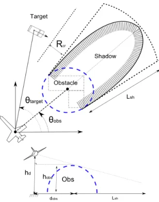
Shadow an area for the target where it is not seen by the UAV (shadows are caused by “visibility obstacles” or “occluding obstacles”), 17
Target The object moving on the ground to be
tracked by the UAV, also called the “evader”, 16
UAV Unmanned Aerial Vehicle, also called the pur-suer, 15
Chapter 1
Introduction
1.1
Motivations
During the past ten years, there has been a significant increase in interest towards Unmanned Aerial Vehicles (UAVs) and this is probably because UAVs have come a long way since their early remote controlled days. Nowadays, UAVs can take off, fly and land almost without any human intervention. Following this trend, global production of UAVs has increased as well: while in 2004, the global production of unmanned aircraft systems (UAS) produced 477 different types of UAVs, some civilian but most military and by 2007 that figure had increased almost by 65% reaching the figure of 789 [International, 2007].
Some of these platforms are by all means impressive: they address many important issues such as flying capabilities, airspace integration, air worthiness and operational capacities. However, they seem to be missing one very important: autonomy. There is often a miscon-ception that as a UAV has the capability to fly by itself during some parts of its mission, it is autonomous. The distinction should be made immediately: on the one hand, automatic flight offers a system the capability to perform actions according to a set of predefined rules in a highly predictable environment, a classical example being the automatic pilot. Whereas on the other hand, true autonomy offers a drone the capability to act without any supervision in an environment that changes and that can face a wide range of conditions. An autonomous system should provide an interface with a very high abstraction level, where the user could command the aircraft to ”Explore(Area)” or ”GoTo(City)” and the system could be left com-pletely unsupervised to perform these tasks. In order to get an idea on the level of autonomy that modern UAVs provide, we should note that for most aerial platforms produced today, the plan following a communication loss is to command the aircraft to go to some deserted area and perform circles until communication is re-established or until all fuel are consumed and the aircraft hard lands.
UAVs have slowly evolved from piloted aircraft and no matter how fast they can fly or maneuver, they still bear a lot of similarities with their piloted counterparts: there is still somewhere a pilot taking the decisions and pulling the strings and the fact that he is not on the aircraft does not change much. On the other hand, robotics research has advanced significantly the past years and it can now offer many elaborate solutions in artificial vision, path planning, decision making, obstacle avoidance and environment modeling – all these work aiming at endowing mobile machines with autonomy. One of the leading motivations of this thesis is to examine the technologies leading to UAV autonomy and attempt to expand
Figure 1.1: Aerosonde: First robotic aircraft to cross the North Atlantic.
some of them.
The second motivation comes from the nature of most UAV applications. They come in a widening range: airborne surveillance, military information gathering, military offensive actions, automated search and rescue, gas pipe line monitoring and automated forest fire surveillance. The common point to most of these applications is that they are defined with respect to the ground environment: ground target tracking, be the target static, slowly moving or maneuvering at high speeds, is an essential task for UAVs. For such tasks, fixed wing UAVs have the advantage over helicopters to reach high speeds at low energy consumption, but their dynamics constrain the visibility of the ground target. This thesis considers this issue, and introduces various strategies to achieve ground visual target tracking, aiming at maximizing the target visibility.
1.2
Challenges and objectives
1.2.1 Problem characteristics
The overall objective of this thesis is to provide methods to endow a drone to autonomously track a moving ground target, under the following conditions:
• UAV dynamics: we consider fixed wing UAVs. This type of aircraft has motion limita-tions and dynamic constraints, and behaves as a non-holonomic vehicle. A fixed wing aircraft cannot stop and change direction as easily as a ground target can do and this raises difficulties, leading to the UAV being out maneuvered by the target. Also, we consider that the UAV motions are constrained by the presence of no fly zones.
• Presence of obstacles: UAVs are unlikely to be allowed to fly over all areas and in the case of a low flying micro drone this assumption is more than often true. One should consider that there exist areas over which the drone cannot venture either because they are tagged as no-fly-zones (NFZs), or because there are buildings to avoid. In any of the above cases one should find ways to pilot the drone in such a manner that it will maintain visibility without entering in the NFZ.
• Field of view restrictions: in many cases, UAVs and especially micro-drones do not have a full Field of View (FOV) leading to a greater complexity of the problem. We will examine the consequences of field of view restrictions for the UAV (panoramic full field of view with respect to limited field of view).
• Target dynamics and behavior: The target may be either moving on an open field or on a road network, and also has dynamic constraints (the model used in this thesis is that of a car). It can be neutral or evasive: in the latter case, it can exploit the presence of obstacles, denoted as “shadows”, to avoid being seen by the UAV, making the problem akin to a hide and seek game.
1.2.2 Thesis objective
Overall, there is a need for the UAV to anticipate the movements of the target in order to be ”a step ahead”. This brings the interest to the level of the decision process: a target that is evasive is going to actively attempt to hide behind obstacles and use the road network in a predictable way. In order to maximize its visibility time, the UAV(s) must be able to predict such situations and to react or plan before they even happen in order to maintain visibility.
The objectives of the thesis is to provide a decision framework that maximizes the target visibility under all these constraints. Additionally, the case of two chasing UAVs will also be considered.
1.3
Contributions and Thesis Outline
The main contributions of this thesis are:
• The presentation of a control based navigation method that permits a UAV to track a ground target, in the absence of obstacles and shadows
• The presentation of a predictive method that permits a UAV to track a target based on its position, while avoiding obstacles and areas that the target can use as hiding places. The method considers the case of an evasive target that moves either in an off road environment or within a road network, and is extended to the case of two cooperative drones.
• The presentation of a discrete game theoretic approach that permits a UAV to track a target based on its position among NFZs and shadowing obstacles, and the extension of this approach to a two UAV collaboration scheme.
1.3.1 Outline
The thesis is structured in six chapters:
• In the second chapter, we review the state of the art on problems similar to the one at hand.
• In the third chapter, we present the problem details, i.e. the numerical models and constraints that we use.
• The fourth chapter presents a method that maximizes visibility under the assumption of a neutral target and a limited visibility, using a reactive navigation approach. • The fifth chapter introduces a predictive method that tracks non cooperative ground
targets, in an environment with obstacles and shadowing obstacles.
• The sixth chapter tackles the same problem, but using an approach based on classical game theory.
• Finally, all implementation tools used during this thesis are briefly presented in annex A.
1.3.2 Implementation Grid
Most of the control based methods presented in the state of the art as well as the one presented in the fourth chapter are rather control based and thus reactive. The methods presented in the planning section of the state of the art as well as the approaches proposed in chapters 5 and 6 are more planning based. The figure 1.2 presents how we locate our contributions in two dimensional “problem complexity” / “solution abstraction” space:
Figure 1.2: Location of our contributions with respect to the state of the art. Note that this figure does not measure the effectiveness of a method, it only illustrates the tackled problem complexity and the solution abstraction.
• “Problem complexity” qualifies the number of constraints to satisfy. For instance, a single UAV tracking a single passive target in an open environment is much less complex than 2 UAVs tracking an evasive target in an urban environment.
• “Solution abstraction” denotes the capacity of a proposed solution to be applied in a wide variety of applications. Low abstraction means a solution tailored to a very specific problem, e.g. a given UAV with a specific FOV, whereas a high abstraction solution mean that it can cope with numerous different problems, such as game theory, which can be applied in economic theories as well as in UAV ground tracking.
The approach proposed in chapter 4 consists of a double control loop that commands a trajectory that permits to the drone to maximize visibility. It tackles a problem a bit more constrained problem than the usual control-based approaches. It however is restricted to open environment, for UAVs with a limited FOV.
The approach presented in the fifth chapter is based on predicting and evaluating future UAV/target configurations to select the action that yields the most satisfying results. It is located a bit more left than the planning solutions on the figure because it has not been proven to work in very dense areas. It however does not require any preplanning, an adapts more easily to the problem as long as mission criteria remain the same.
Finally the game theory approach presented in chapter 6 relies on transforming the con-figuration to a game and then proceeds to find out the best game concon-figurations by using classical game theory tools. It can easily be used for any kind of robotic applications. It is though more on the left than some other applications, because in complex environments, the Nash tabu search will not give always the best solution.
Chapter 2
State of the art
This chapter presents work that has been done in domains that are closely related to this thesis. One must remember that research on UAVs has involved experts from different and distinct domains. However, most early research programs on UAVs were traditionally attached to aeronautics university departments and as a result all experts involved at those programs where some-how related to Guidance, Navigation and Control fields. The result was that those researchers produced solutions heavily influenced by their research fields. As technology on UAVs was evolving, the cost and complexity of UAVs greatly diminished, and powerful and easy-to-use simulators can now be used by almost anyone having a personal computer. This makes it easier for researchers without any aeronautics background to enter the race: robotics and artificial intelligence researchers seized this opportunity. With their elaborate algorithms and with their iterative solutions, they not only provided new ways to tackle the UAV problems but they also produced new tools.
• The first body of research, is based on Guidance, Navigation and Control. It’s main interest is how to change a trajectory in order to achieve maximum visibility of the target. Most of the scientific papers published in this domain also deal with the control aspects of the problem. However, very few deal with the presence of No-Fly zones or any other type of visibility obstructing obstacle. The typical scenario is the following: a target moves in an open field, while the UAV flies at a steady altitude and with steady speed, while trying to remain close to some ground target.
• The second body of research draws its forces from planning based solutions and moves a step further to autonomy.
• The third type of work presented in this chapter is game theory, that has been his-torically one of the most influential in the domain of decision making.
• This chapter would be incomplete without a presentation of multi agent environ-ments and the two main type of interactions that can arise: competitive interac-tions in the sense that target and UAV try to outsmart each other and cooperative interactions in the sense that two or more UAVs may cooperate to maximize some common utility.
2.1
Guidance, Navigation and Control
The first Unmanned Aerial Vehicle to ever fly autonomously was the Hewitt-Sperry Automatic Aeroplane, also known as the ”flying bomb” [Pearson, ]: it performed its first flight on 12 September 1916. Its control was achieved by the use of gyroscopes and signaled the start of the UAV era. For the following forty years, the research on UAVs remained essentially a research on control theory. We could define this period as the control and guidance problem phase of UAV research. The question that researchers were seeking to answer was the following: How can one make an unmanned aircraft closely follow a predetermined heading, altitude and speed ?
As electronics and control theory evolved fast, this problem soon became trivial and led to a new research phase for UAVs: What kind of system should we use on an aircraft, in order to be able to get from point A to point B successfully and without any form of direct human control ? This problem was known as the navigation problem and it was especially interesting when point B was moving.
2.1.1 Waypoints VS Continuous Navigation
The guidance, control and navigation methods can be divided into three different approaches: • In the waypoint approach, every trajectory is first divided into a series of waypoints that the drone must attain. Each waypoint is reached, one at a time, before the next waypoint is fetched from the list. As a result, any desired trajectory must first be divided in a series of waypoints before it is fed back to the control level.
• On the other hand, in continuous navigation approaches, waypoints are not neces-sary at all. Instead, a continuous stream of commands is passed directly to the control level. Most visual servoing [Bourquardez and Chaumette, 2007] and missile guidance approaches fell under this category. As every guidance law is tuned to optimize some problem specific criterion, there doesn’t exist any generic method for Continuous Nav-igation control and as such each problem has to be treated individually.
• There exists also a mixed third type of approaches: mixed strategy. This approach makes use of both characteristics and shows quite good results in terms of trajectory following.
2.1.2 Missile Guidance
There are many similarities between UAV guidance and missile guidance. There exist many missile guidance laws that can assure that, a missile starting from a position A can most times hit an evading target B, with a reasonable probability.
Missiles are relatively simple flying machines that fly at a maximal (and most of the times, not controllable) speed. Even if there exist missiles that change their speed as part of their strategy, in most cases the missile guidance problem involves one control variable only: a force αm applied normally on the missile’s vector Vm. When the missile reaches a critical
distance from the target, it detonates and this is known as a capture.
Figure 2.1: This is a 2D graph of Proportional Navigation applied on the lateral plan.
Proportional Navigation (PN) (Fig. 2.1) is one of the oldest and most classic method used by missiles in order to capture targets. The idea has been proved to work so well, that it remains still in use today, five decades after its first appearance in scientific papers.
PN is based on the fact that two vehicles are on a collision course when their Line-of-Sight (LOS) angle does not change. In order to achieve that, the normal angle αm remains
proportional to the rate of change of the LOS ˙ρ, using the following formula: αm= N ˙ρ
N is a gain that permits to tune the behavior of the missile trajectory: a gain of N = 1 yields a curved trajectory, while a gain of N → ∞ guides the missile straight to the position of the target with no curvature1
Pursuit Guidance (Fig. 2.2 (a)) is a very simple method that makes sure that the missile always flies towards the evading target. Even if this method can some times be impractical for closing the final distance and ’capturing’ the target, it still remains an excellent method for approaching closer to the target.
Deviated pursuit Guidance (Fig. 2.2(b)) is quite similar to the pursuit Guidance with one significant difference. The missile angle leads the LOS angle with a fixed angle λ. This is like anticipating where the target will be and thus covering less distance than the target.
Three Point Guidance (Fig. 2.2(c)) makes sure that the missile will always lie some-where between the target and the target tracker. It is known also as constant bearing guidance. For a good introduction on these methods, the reader might want to look at the classical work of Siouris [G.M.Siouris, 2004]. For more details, in [M.Guelman, 1971] one can find a good study on Proportional Navigation in one of the oldest publications that exist on the subject. [D.Ghose, 1994] and [Yang and Yang, 1997] treat the problem of a maneuvering target and they show how proportional navigation achieves capturing evasive targets. Finally, in [U.S.Shukla and P.R.Mahapatra, 1990] an alternative method of PN is presented, where the applied force is not normal on the missile speed vector, but on the LOS vector instead.
One very interesting application of PN on a wheeled, ground robot is given in
[F.Belkhouche and B.Belkhouche, 2007], where the authors use a more relaxed version of the law:
1The curvature should not be confused with unwanted oscillations that may arise. A missile can move along
Figure 2.2: Different forms of missile guidance.
θR= N ρ + λ
where θR is the robot heading with the reference frame, ρ is the LOS angle and λ is the
lead angle that if different from zero can have the same effect as in deviated pursuit guidance. It should be noted that during the simulations the robot manages to find its way in the presence of obstacles.
2.1.3 Mixed strategy trajectory following
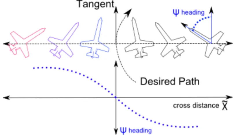
Nicolescu [Niculescu, 2001] proposed a lateral track law that manages to hold a UAV very close to its trajectory. This approach, behaves very well in straight lines. However, a method that could behave well both on straight lines and on curved trajectories was proposed by Park et al in [Park et al., 2004].
Park (Fig. 2.3) proposed a nonlinear guidance law that performs better than conventional Proportional Derivative controllers. This approach has been shown to be mathematically equivalent to a PN guidance law with a gain of N = 2.
The law of the guidance law is:
αcmd = 2
Vd
L1
sin η
where αcmd is the lateral acceleration command, Vd is the drone speed, L1 is the distance
between the reference point and the drone and finally η is the angle between the drone speed vector and the UAV / reference point LOS. The method has been used for obstacle avoidance as we will see later in [Ducard et al., 2007].
Figure 2.3: Diagram of Shangyuk Park’s proposed guidance law.
Figure 2.4: Diagram of the ’good helmsman’s’ Guidance.
2.1.4 Waypoint Guidance
One of the most classic methods in the UAV Guidance literature, comes from waypoint tracking control of ships [Pettersen and Lefeber, 2001]. The idea behind this principle is to model the behavior of a ’good helmsman’ (Fig. 2.4), the person that has the task to steer a ship, a submarine or any type of maritime vessel. The idea was presented to the UAV community by Rysdyk in [Rysdyk, 2003], who fine tuned it for the aircraft case.
2.1.5 Potential Fields
These methods use repulsion from undesired configurations and attraction towards goals in order to compute a path. A useful method to generate motions is the Potential Field (PF) (Fig. 2.5) [Latombe, 1991]. The primary advantage is that PF approaches were developed for real time applications. The idea behind PFs is that every point, which has to be avoided is surrounded by a repulsion field while every desired goal point is surrounded by a attraction field. This way the robot will move around the obstacles that repulse it and move towards the points that attract it. Using this simple formulation the task of path planning becomes much easier: the robot always moves towards the area that attracts it the most and this can be done using any greedy local search method like e.g. steepest descent. A similar approach
Figure 2.5: Trajectory of a robot that avoids two obstacles while heading for some distant goal with using a Potential Field method.
uses probability density functions as evaluations functions [Dogan, 2003][Kim et al., 2008]. However, the biggest caveat of this method is that robots can be easily trapped into local minimum and remain there in the absence of an external aid [Koren and Borenstein, 1991]. A good mechanism to break cyclic behaviors is proposed in [Dogan, 2003]: Every time a change in UAV heading is detected a counter measures how much the aircraft has turned: If a full 360 degrees heading change is detected, the behavior is noted as cyclic and the aircraft enters an exiting pattern. Another solution proposed for overcoming cyclic behavior in potential field methods is the change of altitude [Helble and Cameron, 2007].
2.1.6 On Non-holonomic Aircrafts and Time Optimal Paths
Aeroplane dynamics are constrained by various laws, spanning from aerodynamics to struc-tural engineering. However, the most influential law for target tracking are those of lateral movement, as they can help the selection of a UAV optimal path.
A robot whose configuration space has l dimensions is a non-holonomic robot, if it is constrained by k non-integrable constraints Gi with i ∈ k and (0 < k < l) of the form :
Gi(q, q0) = 0
An aeroplane behaves exactly as a Non-holonomic vehicle when it is examined with respect to its lateral movement. A Non-holonomic vehicle is a vehicle whose current posture (position and orientation) depends on the path it took to get there.
The model that seems to correspond the most is that of the Dubins car as it is known in the Robotics community from the ground breaking work of L.E.Dubins [Dubins, 1957], published in 1957. 2
2
However, what until recently was not known is that, another researcher under the name of Pecsvaradi published a paper in 1972, covering the same aspects, arriving at the same results and focusing solely on aeroplanes. However, as he published in a journal that was read almost only by researchers from the Control and Guidance community, his work did not reach the Robotics community, until very recently. The two researchers arrived at the same results but did it using two different approaches: Pecsvaradi used the Pontryagin Maximum Principle (PMP) and found what guidance law is appropriate, when an aircraft wishes to get from one point to another, in a time optimal manner. On the other hand, Dubins achieved the same result but this time using Topology elements, without mentioning the application. For a good introduction on PMP , one can read [L.M.Hocking, 2001] and for an introduction on Topology, one can look at [Lipschutz, 1968].
The term Dubins Aircraft was coined in [Chitsaz and LaValle, 2007], where three dis-tinct cases where examined all using the Pontryagin Maximum Principle (PMP): what are the time optimal paths in order to attain three different goals of low, medium and high al-titude. This type of work has been applied for years in the Robotics community in order to find optimal paths for ground robots. Good examples can be seen in [Bui et al., 1994] and [Tang and Ozguner, 2005].
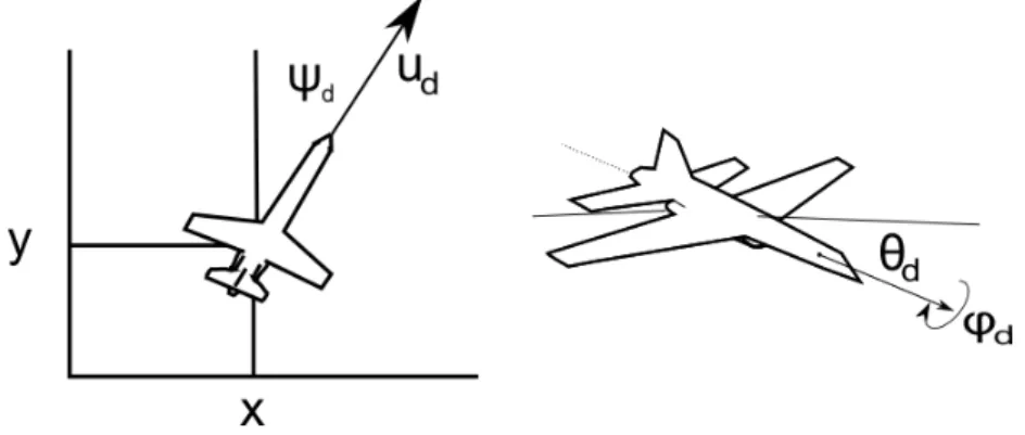
The model of the Dubins aeroplane is given by:
˙ x = v cos ψ (2.1) ˙ y = v sin ψ (2.2) ψ = −(g/v) tan φ (2.3) (2.4) where x and y are the Cartesian coordinates of the aeroplane, ψ is the heading angle of the aeroplane, v is the speed of the aeroplane, φ is the bank angle and g is the gravity acceleration. It should be noted that the bank angle is bounded:
|φ| ≤ φmax
For any aeroplane (or robot) following the above equations, any given initial and final configuration can be attained using six types of paths (Fig. 2.6), constructed from three arcs only. This means for every UAV, moving in the absence of obstacles, only three type of commands are necessary to attain any point on the horizon under any type of heading:
• An arc of a counterclockwise, left circle (L) ψ = −(g/v) tan φmax • An arc of a clockwise, right circle (R) ψ = (g/v) tan φmax
• A straight line segment (S) ψ = 0
2.1.7 UAV Trajectory Optimization for Target Tracking
Target tracking includes a series of methods that permit a UAV to bring in or to maintain the target within its camera frame. This is done by adjusting accordingly the UAV trajectories and camera postures in order for the drone maintains target visibility. The key aspects of these methods are to maintain target proximity and proper camera orientation.
Lee et al [Lee et al., 2003] propose the following strategy in order to track a ground target: the UAV enters in two different modes accordingly to the speed of the ground target. If the target moves too slow, then the UAV enters a loitering mode that looks like a rose curved trajectory (Fig. 2.8) and by this it remains close to the target. If however the target starts to move faster, it enters into sinusoidal mode. During this mode the UAV follows a sinusoid wave pattern trajectory, whose frequency and amplitude depend on the targets speed and thus staying close to the target. The target’s position is supposed to be known already, while a full FOV visibility is assumed for the camera. The authors have proved the functionality of the algorithm in a real flight test.
Stolle et al [Stolle and Rysdyk, 2003] make use of the helmsman’s guidance law in order to track a ground target. They examine different types of camera visibilities and provide
Figure 2.6: Two examples of optimal trajectories for a Dubins aeroplane. Note the different headings of the waypoints.
Figure 2.7: Different configurations of cameras. We can see cameras that are of static, roll only and pan-roll, depending of their capabilities to turn on certain axes. β is the roll (or tilt) axis and α is the pan axis
different type of trajectories. They show that for a full FOV camera, a circular path around the target will guarantee visibility. However, when the camera has limited camera angles (Fig. 2.7) and it is in the presence of wind, they propose to add a sideslip angle in order to maintain the target within the camera FOV without changing flying path. They remark the negative effects of the sun and the wind and they propose segmented circular orbits (Fig. 2.8) around the target of different radius in order to avoid the angles where visibility is deteriorated.
Figure 2.8: Different strategies for tracking a ground target.
Husby during his master thesis added a square wave pattern trajectory that achieves the same result as the sinusoidal method and demonstrated that the methods presented in [Stolle and Rysdyk, 2003] work equally well with moving targets.
The case of a roll only camera (Fig. 2.7) has been examined in [Thomasson, 1998] by Thomasson. He proved that for such a configuration only three type of trajectories are viable: spirals, circles and ellipses, all depending from the wind vector. He then provided the guidance laws required for a UAV to perform a search. The author of [Rysdyk, 2003] decided to work on a ’clock-angle’ frame of reference, with each algorithm evaluating every bearing angle around the UAV. This time the camera is considered to be of pan and roll type (Fig. 2.7). The author looks for the trajectory that maintains the geometry between target and drone constant. He then arrives at results similar the roll only camera case. The idea of an ellipse trajectory that compensates wind presence has been examined in [Sun et al., 2008], where the authors described the pan, roll camera guidance law. Also in [Rafi et al., 2006] the authors propose a circular pattern around a target and offer the guidance algorithms to achieve that.
In [Quigley et al., 2005b] the authors proposed an attraction field generated by a super critical Hopf bifurcation in order to keep the UAV close to the target. A Hopf bifurcation is a phenomenon appearing to certain dynamical systems, causing a limit cycle attraction field. An interesting application of the Dubins aeroplane in order to follow a slower target (in this case a helicopter) has been presented in [Ryan and Hedrick, 2005] where the methods reminds us the work on sinusoidal guidance, seen earlier. In [Rathinam and Sengupta, 2004] the authors assume that a fast moving UAV will not have the time to scan the areas for threats. So they propose to delay the forward speed using circle trajectories in order to scan the area.
2.1.8 Synthesis of Guidance, Navigation and Control Bibliography
Missiles, drones and cars all behave as non-holonomic vehicles and as such any law that can guide successfully one type of engine can guide another one too – when we examine them in the lateral plane. Missile guidance laws provide a good set of tools that can permit a UAV to approach a target, a waypoint or a trajectory path. In essence this is what Sanghyuk guidance
achieves, as under some circumstances, it closely resembles to proportional navigation. It was shown that for any UAV, three commands are enough to successfully plan a path. This can be of great use when graph search algorithms will be implemented.
In the domain of reactive path planning there exist numerous trajectory patterns that can achieve a good observability. However, these methods depend from the type of camera:
• For roll only cameras, Ellipses and Circles seem to be the trajectories that provide a good target visibility through the trajectory.
• For full FOV cameras, a circular path seems to track the target the best.
• For 180 degrees FOV cameras, a circular path may not be good enough in the presence of wind, as it can easily throw the target out of view. Two solutions are proposed: Either add a sideslip angle if that option is available on the drone or perform an ellipse based trajectory.
These trajectories are actively constructed with predefined patterns by examining the Cartesian coordinates of the drone. The knowledge of when to switch from one type to another is assumed to derive either from the position of the drone or from measuring its speed. Very few of these cases consider an obstacle that obstructs either the UAV path or the target image. As a result they can function only under special conditions.
Furthermore there doesn’t exist a comparison that can show us which of these methods presents the best target tracking score under different target movements.
Another point that varies significantly is the way the target’s position is acquired. In most cases the position is known via some external source and very few actually test the method with a real flight camera feedback.
Overall, there seem to exist several methods that address the visibility issues but there lacks a unification, a single method that can be used in all of the above combinations of camera types, target position input types and aeroplane types.
2.2
Planning based methods for UAVs
Some of the methods examined in the section are:
• The use of predictive methods in order to select the best future path.
• Research of all possible configurations in order to find the best path possible using search algorithms.
• Anticipation of target movement in order that the drone will position itself in such a way that it will be easier to track the target, even if the target tries to avoid capture. This capability falls under the category of adversarial searching and the applications arising are known as pursuit evasion games.
2.2.1 Path Finding for UAVs
Path or Motion Planning in Robotics, is the process where a machine produces a collision-free path from a point A to a goal point B. However, this section does not address only methods that pre-plan a path, but also expands to methods that simply search to find a near optimal path under several constraints as obstacle avoidance and target visibility (Fig. 2.9).
Figure 2.9: Summary of the tools and application domains presented in the Path Finding bibliography.
2.2.2 Search algorithms
Despite the real world fluctuations, in the AI world drones are considered to be flying in a 3-D space known as a State Space.
The problem as it is proposed by Path Planning is: What kind of process should a machine use in order to find an optimal path starting from an initial state towards some desired goal. Most search algorithms used in the Robotics literature are mainly of graph search type. [Russell et al., 1995][Korf, 1985] The basic idea behind graph search algorithms is to use the nodes of a search graph to store information for every state space available. Each node also stores information regarding the path cost one would use to get to that node, based on problem related criteria. This way the question of path planning becomes a question of finding the optimal path within the search tree. After one node is examined and found that it is not the goal node, all or some of its descendant nodes are generated and examined in order to see, if any of them is the goal node. The total cost of each candidate path is the sum of all individual costs of every node participating in the path. Here, some complexity issues arise as the search tree expands (also known as the depth limit or diameter of the graph), so do the calculations necessary to complete the process. For an on board computer, this may bring up issues of memory usage and processor time allocation.
There exist two main categories of search algorithms:
• Informed methods use some form of heuristics in order to select which node will they open.
• Uninformed methods where no information exists concerning which node should the algorithm explore next. As a result nodes are opened one by one until an end goal is
reached.
Uninformed search algorithms
In this category we find the following algorithms: • Uniform-cost search algorithm
• Breadth-first search algorithm • Depth-first search algorithm
• Depth-first iterative deepening search algorithm Informed search algorithms
• Branch and bound search algorithm • Dijkstra’s search algorithm.
• A* and all its descendants (IDA*, D* etc) • Steepest Descent search algorithm
Example 2.1.
Local search algorithm - Tabu search
The tabu search method is an optimization solution that uses local search methods. This specific search method overcomes local minimum by using a special memory structure known as the tabu list T . As the algorithm proceeds evaluating different solutions using some termina-tion conditermina-tion, it places in the tabu list all solutermina-tions that it has already examined. Once a solu-tion is put in that list the algorithm can no longer reuse it, forcing thus the algorithm to search for new, alternative solutions. When the algorithm is applied to a graph this leads to constantly exploring new paths until a solution is found [Gendreau, 2003, Glover and Laguna, 1993].
Example 2.2.
Heuristics graph search - for Robots
A* algorithm is a widespread search algorithms used in Robotics and AI. It is used to find the least cost path from an initial node to the desired end goal. It is a best first, informed search algorithm. While most algorithms will expand all nodes one by one until they arrive to the end goal, A* uses a shortcut in order to arrive to the end goal. This is achieved using an evaluation function f (x) that helps select only the most promising nodes to expand. For this reason, the algorithm keeps in memory a whole front of nodes and keeps expanding only the best one at a time. Once a node has been examined and found not to be the end goal, it is
removed from the front and its successors are placed in memory, restarting the whole process again.
The evaluation function f (x) of every node consists of two parts:
• g(x) where the cost of the path from initial-node-to-the-present-node is stored. • h(x) a Heuristic function where the estimated-to-the-end-node cost is stored.
In order for A* to be optimal an admissible heuristic h(x) is needed, something that can be achieved if the heuristic underestimates the actual cost left to reach the goal. In other words, this means that the heuristic must always be optimistic and a way to do that is by adopting a relaxed version of the problem. In the case of a robot that seeks to find the shortest path to a goal, the Cartesian distance between the node in question and the goal is admissible.
Figure 2.10: Diagram of a robot that uses A* for path planning.
Furthermore A* is complete, meaning it will always find a solution if there exists one. The worst case for time and space complexity is O(bd) where b is branching factor or the
maximum number of successors of any node and d is the depth of the goal in steps. Fig. 2.10 shows a robot using A* while trying to find the shortest path to some desired goal.
2.2.3 Variants of Potential Fields
Another local method that avoids some of the local minimum problems is the vector field histogram (VFH) [Borenstein and Koren, 1991][Ulrich and Borenstein, 1998]
[Borenstein and Koren, 1990]. This approach constructs a polar histogram containing a value representing the polar obstacle density in every direction. As the method is bearing oriented as opposed to Cartesian position oriented, it can avoid some forms of local minimum. However, this can lead to dead-end situations and exhibit cyclic behaviors, where the robot moves from one obstacle to another.
2.2.4 Path Finding and Obstacle Avoidance
A classical approach to ground robot path planning is the construction of a traversability map [Singh et al., 2000] [Gennery, 1999] followed by a graph search method to find the best route to the desired goal.
A related method is the arcs approach [Lacroix et al., 2002] [Langer et al., 1994], where a series of arcs is generated and compared one to each other in order to select the one with the least cost. The robot then chooses steers along its way. The cost function is the sum of traversability values along its path. This type of search is called greedy as instead of searching a sequence of commands along the way, it selects the immediate best command. It is situated somewhere between control and planning.
A commonly used method is that of behavior based algorithms [Langer et al., 1994] [Seraji and Howard, 2002] where every task in the path planner generates its own heading and speed setpoints. In the case of a conflict a behavior arbitrator fuses the different setpoints and finds the common decision.
The organization of path geometry around obstacles is also a quite important subject in robotics. A very common technique is the use of Voronoi graphs [Latombe, 1991]
[Barraquand et al., 1992] to find the routes between obstacles. Voronoi graphs are used to separate the neighbor areas from two or more obstacles at equal distances. In UAVs this has been applied in [Bortoff et al., 2000][Chandler et al., 2001]. This method permits to find a safe path among two or more obstacles. A very closely related method is the separation of the space with the Finite Element Method [Pimenta et al., 2005].
A method that searches a route among obstacles is the Roadmap method [Latombe, 1991] [Isler et al., 2005]. The method creates a graph consisting of lines connecting all edges of an object (or tangents leading to the object) including: the end goal, the obstacles positions and the robot position. It then proceeds at finding the optimal path at that graph. In [Isler et al., 2005] this is done in order to minimize time.
In [Rathinam and Sengupta, 2004] the authors use the Dijkstra’s algorithm along with a risk map in order to navigate the drone through safe areas. Finally, a very good application of Park’s lateral guidance law was proposed by Ducart et al in [Ducard et al., 2007]. The authors proposed the use of tangent lines starting from the drone and touching the security circle around the obstacle. The points of contact are then used as waypoints for the lateral guidance law and drive the UAV around the obstacle. This method can be very useful in the case of a drone that is moving and detecting obstacles in real time as it does not need beforehand trajectory calculation.
Another method that is lately gaining a lot of ground is that of Rapidly-exploring Ran-dom Trees (RRTs). This method permits to perform a research in highly multidimensional
Figure 2.11: Trajectory of a robot that avoids an obstacles, while heading for some distant goal with the use the method proposed in [Ducard et al., 2007].
non convex areas and in drones is applied by exploring random arcs and then choosing the ones that are the closest to the end goal and not in contact with any obstacles. RRTs perform really well with path planning problems that involve obstacles and differential con-straints. Work on RRTs can be found in [Tan et al., , LaValle, 1998, Bruce and Veloso, 2003, Kuffner Jr and LaValle, 2000].
2.2.5 Synthesis of planning methods
The basic tool presented in this section involve variants of potential field methods and graph searching tools. Robotics provides a set of tools that allow any type of robot to navigate from one point to another, while avoiding any obstacles that it may encounter. Overall, we can consider that the solutions are robust enough and with some slight changes they could be used for fixed-wing UAV path finding. However, one should not forget that fixed wing UAVs have two very important constraints: in contrast to ground robots and helicopter UAVs, they cannot stop. Furthermore, small UAVs may have computation limitations. The work that should be done in this domain would be to adapt somehow the above methods in order to produce a fixed-wing UAV path-finding algorithm that respects the above constraints.
2.3
Decision: game theory
This section deals with a basic analytic tool of decision theory. Decision theory is a framework that permits one to take the best decision under a set of rules and based on the information that the decision maker has at a given moment.
Game theory: introduction
Game theory [Fudenberg and Tirole, 1991, von Neumann and Morgenstern, 1953] is a branch of applied mathematics that tries to capture behaviors in strategic situations as the ones en-countered in multi-agent environments. It deals with the decisions that an individual or a team has to take, when its success depends on the choices of others. It has applications that
span in various domains: social sciences, economics, biology, engineering and political science being some examples.
Example 2.3.
Game theory: Quick Review
A game G is a mathematical object that describes the interaction of a group of players i ∈ N , where N = 1, ..., n is the set of players. Each player can choose among a set Ai of
actions σi ∈ Ai (aka pure strategies) or among a set of mixed strategies ∆(Ai). Furthermore
the player is considered to be rational and thus seeking to optimize a certain utility or payoff ui: A → <.
Games can be found in different categories depending on several parameters:
• Cooperative vs non-cooperative games. In a cooperative game, players can form coali-tions, as opposed to non-cooperative games, where each player is trying individually to optimize his own utility.
• Zero sum vs non-zero sum games. A zero sum game is a game where the sum of all payoffs of all players is equal to zero: PN
i ui = 0.
• Sequential vs simultaneous games. During simultaneous games, both players move si-multaneously as opposed to sequential, where players alternate moves.
• Perfect information sequential games vs imperfect information sequential games. If all players know all actions performed by other players previously, then the game is said to be of perfect information.
• Complete information sequential games vs incomplete information sequential games. In incomplete information games, the players may not know exactly what their or their co - player’s payoffs may be.
• Discrete vs continuous games. When players can choose actions only from a discrete set of actions, then the game is said to be discrete as opposed to continuous games, where players can choose a strategy from a continuous strategy set.
Games can be represented in the following forms:
• The extensive form (Fig. 2.12). Here the games are represented with a tree and each node (or vertex) represents an action (or decision) taken by a player. The payoffs are noted at the bottom of the tree. The extended form can represent both sequential and simultaneous games. For the later case, while one player is moving, there is uncertainty on what the other players are doing. To symbolize this, one has only to connect the nodes with a dotted line where this uncertainty arises – or circle them. The connected nodes represent the possible alternatives of that move and show what information is missing. This is known as the information set.
To put it alternatively, an information set of a certain player P, is the set of all possible moves that could have taken place so far, based on the information that player P may have. For a perfect information game, every such set consists only from singletons: sets that have only one member.
Figure 2.12: A game with imperfect information represented by its extensive form.
Figure 2.13: Normal form of the Prisoner’s Dilemma. Two friends are arrested by the police as suspects for committing a crime. However, the police does not have enough evidence against them and decide to separate them in order to offer them a deal: if one testifies (”betrays” his friend) for the prosecution against the other and the other remains silent, the betrayer goes free and the silent accomplice receives a full 10-year sentence. If the both remain silent, they both receive only six months. If each suspect betrays each other, they both receive five years each.
• The normal or strategic form (Fig. 2.13). Here the games are represented with a matrix and each cell depicts the outcomes of the moves for each player. Within the cell, one marks the payoffs of that combination. This representation is used only for simultaneous games or games of imperfect information.
• The characteristic function form. For games of cooperation, no individual payoffs are assigned but instead one can use a group payoff v : 2N → < for every coalition S arising from a set N of players.
Dominance Strategies, Non-cooperative games and Individual Decisions
An event E is mutual knowledge if everybody knows E. E is common knowledge if everybody knows E, everybody knows that everybody knows that everybody knows E with this pattern continuing towards infinity.
A strategy σi∗ strictly dominates σi (σi∗ σi) if:
∀σ−i ∈ ∆(A−i) : ui(σi∗, σ−i) ≥ ui(σi, σ−i)
In the case of the Prisoner’s Dilemma (Fig. 2.14) the silent strategy is strictly dominated by the betrayal strategy. Regardless, what the other player may choose, a player will be better off if he decides to betray his co-player. However, this can mean that he will be trapped in a sub optimal outcome. This concept shows that rational, selfish decisions are not necessarily optimal for a player.
Figure 2.14: Strong Nash Equilibrium in Prisoner’s Dilemma: Always betray your friend.
∀αi ∈ Ai: ui(α∗i, σ−i) ≥ ui(σi, σ−i)
A strategy profile σ∗ = (σi∗, ..., σn∗) ∈ ∆(A1) X ... X ∆(An) is a Nash equilibrium
[Nash, 1950, Nash, 1988] if for any i ∈ N :
∀σi ∈ ∆(Ai) : ui(σi∗, σ ∗
−i) ≥ ui(σi, σ∗−i)
Coalitions and Cooperative games
A cooperative game is a game where players form coalitions and they compete against other coalitions for some common utility. In a mathematical form every coalition S of a set N of players is assigned a payoff value v : 2N → < describing how much value can a group of players earn by forming that coalition S.
There exist different methods for finding ways to fairly allocate the collective payoff to players of the coalition. Some of those solution concepts are known as the Core, the stable set (known as “von Neumann-Morgenstern solution”) [von Neumann and Morgenstern, 1953], the Shapley value [Shapley, 1953] and many others. However, these methods are interesting when more than two players are involved, something that is not the case for this thesis where only two drones cooperate to guarantee visibility of a target.
However, there exists a concept in game theory that can be of interest for cooperation and that is Pareto efficiency. If one imagines that there is more than one way to distribute a common good or utility to a group of players, then a movement from one type of wealth allocation x to another type of allocation y that augments the wealth of one player, with-out making the situation worse for another player of the coalition, is called a Pareto im-provement: y x. Thus, a good allocation is called Pareto optimal or Pareto efficient [Fudenberg and Tirole, 1991], when no further Pareto improvements are possible within that set of players. The set of choices within a coalition that are Pareto efficient are known as the Pareto frontier (Fig. 2.15) or Pareto set. The Pareto frontier describes the maximum possible welfare for a given group of players. If one returns to the example of the Prisoner’s Dilemma as it was seen earlier (Fig. 2.14), we can see that while the Betray-Betray strategy is a Nash Equilibrium, it is not Pareto efficient and that is why it seems so counter intuitive to us.
Differential games
Classical game theory representations like the matrix form and the extensive form seem to be excellent tools for formulating and proving the basic theorems of game theory but they seem to be unsatisfactory tools for solving real life problems.
Figure 2.15: This graph depicts the Pareto frontier. Each axis is the welfare of a player, in an imaginary game where more utility is best. While decision C is better than decision B for player 1, it is a much worse decision for player 2 as it provides less wealth and thus it is dominated by point B. As a matter of fact, the only decisions that are not dominated by other decisions, are the ones that are on the Pareto frontier. In other words, the Pareto frontier depicts the maximum possible welfare for a given group of players.
Unless the problem is very simple, (e.g. very few players, with few discrete options for each player) the problem matrix becomes astronomically large, quite difficult to track and even more difficult to solve. This is why another method is needed to tackle the problems by analyzing the inner logical patterns of the games and producing some set of equations that one can solve.
Differential games [Isaacs, 1999] is a branch of game theory where players move sequen-tially instead of alternatively, and is mostly used in economic applications. It uses notions as barriers, zones and backward induction to deduce whether a pursuer can ’capture’ an evader or not. In most cases the strategies are not discrete but continuous and in several cases, it can provide the control trajectory and use it to optimally guide a pursuer to a capture.
Classical problems for differential games are battles, pursuit-evasion games, dogfights, football, missiles intercepting aircrafts and many others.
One must bear in mind that in most cases differential games treat two-player zero sum games with perfect information. While there exist differential games that are discrete, for most cases differential games are considered to be continuous. This means, that players are making their decisions by adjusting the values of certain control variables that are the equivalent to strategies from classical game theory.
These decisions affect the values of certain quantities in the game that are known as state variables. These variables contain all necessary information for the game so that if one of the players had to stop and be replaced by a new player during the game, the new player would have all necessary information in order to continue the game from that point on – without an external viewer noticing the switch.
UAV applications for game theory
In [Sujit and Ghose, 2005, Sujit and Ghose, 2004] the authors present a game theoretic method for searching an area using N ≥ 2 drones. As utility they use the uncertainty of the existence of a target in a given area or not.
In [Tomlin et al., 2000, Mitchell et al., 2005] the authors provide an algorithm that based on the above rationale permits to backwards calculate the initial configurations for collision avoidance. In [Reimann, 2007] the author provides three ideas related to differential games. For a multi UAV, multi target scenario he either proposes to decompose the problem in many mono UAV, mono target problems that he resolves using either differential games or the principle of maximum.
2.4
Competitive Approaches
When there are more than one agents acting in an environment and when each agent’s success depends on the other agent’s actions, then we are dealing with a multi-agent environment. The interactions that can arise in such an environment can be either cooperative, neutral or competitive.
Tracking a ground target is a multi-agent environment and in the quest for an optimal decision, the behavior of the target should be taken into account. Here we will consider the case where the target is trying to evade the drone and as such it enters in the context of game theory, the game being a zero-sum game [Fudenberg and Tirole, 1991]: if one agent wins then the other one loses. The notion of winning and losing is evaluated using an evaluation function which is tied individually to each problem i.e. a common class of problem is that of pursuit-evasion games, where one group tries to track down another group in a given environment. Even more both targets are considered to be rational players: they both seek to play optimally.
Pursuit evasion games
Any problem that involves a group trying to track down another group is called a pursuit evasion game. In UAV literature the solutions for this class of problems could be divided in two types: theoretic based and planning based approaches.
the most widely planning based method is a control method known as Non Linear Model Predictive Control (NMPC). It was used in robotics for the first time in 2000 as an application for an autonomous submarine that could follow the seabed at a fixed depth.
[Sutton and Bitmead, 2000]
NMPC is a method that was originally designed to be used for control of non-linear processes using a predictive iterative optimization. It consists of a two step loop:
1. First, a non-linear model projects the future state of the process using the optimal command found during the previous iteration,
2. An iterative optimization method based on Lagrange multipliers and steepest descent gradient optimizes a certain cost function, deriving the command that will be used during the next iteration.
[Kim and Shim, 2003], helicopter obstacle avoidance, helicopter autonomous navigation [Shim et al., 2003][Lee et al., 2003][Shim et al., 2005] and path finding for a swarm of ground vehicles in the presence of obstacles [Xi and Baras, 2007].
The above iterative optimization step can be replaced and one can instead use an approach based on either Mixed Integer Linear Programming [Richards and How, 2003] or Convex Quadratic Programming [Singh et al., 2001] to derive the optimal command. These methods have been applied in spacecraft rendez-vous, automated air traffic control and autonomous ground robot navigation applications.
Autonomous pursuit is a class of applications where an autonomous drone tracks one or multiple targets in the presence of areas with threats, obstacles and restricted zones. One approach to this class of problems is the use of a state prediction in combination with a rule based method [Zengin and Dogan, 2007].
Studies that examine visual pursuit include the work presented in [Muppirala et al., 2005], where the pursuer and evader are considered to be connected with an imaginary fixed length bar. This way, the problem is transformed to a motion planning problem with sole goal to find a trajectory where the bar does not touch any obstacles.
However, in all the above cases it was considered that the UAVs have a complete FOV which often is not the case. There exist methods that show analytically a way to perform tracking using pursuit-evasion games [Bopardikar et al., 2007] for ground robots having only disk visibility. The theoretic case of search under limited visibility has been given an analytic solution in [Gerkey et al., 2006].
Adversarial searching
Adversarial search is a process that seeks to find the optimal decision for one player, while taking into account the actions of its opponent. This is done by trying to get the Minimax value, which is the best achievable payoff against the best possible play of the opponent. The algorithm that achieves that is the Minimax algorithm which is known to be complete, optimal (if the opponent is rational), it has a time complexity of O(bm) and a space complexity of O(bm) for depth first exploration – with b being the branching factor and m the depth of the calculations.
Another well known method is α − β pruning. It ignores the nodes of the of the search tree that do not influence the final decision. This way it is possible to compute the correct minimax decision without having to process the whole search tree.
Example 2.4.
Chess and adversarial searching
Few games have been studied as much as chess. In May 1997, news circled the globe that world champion Garry Kasparov had been defeated by a computer. The machine, named Deep Blue, apart from a massive parallel array of processors and custom made VLSI chips, used adversarial searching as its core algorithm. Deep Blue used an iterative deepening α − β pruning searching algorithm [Campbell et al., 2002] [Marsland et al., 1991] that permitted it to calculate an average of 126 million positions per move in a game that has a search branching factor of 35, leaving no place for resource allocation errors. Only the evaluation function, included 6000 to 8000 features. To enhance this effect, it searched the top levels of the chess tree, examining interesting positions and developing them beyond the standard processing horizon [Campbell et al., 2002].
Figure 2.16: During the last, famous sixth game, world champion Garry Kasparov loses against IBM Deep Blue computer.
Minimax [Norvig, 1992] is an algorithm used very often in adversarial searching. Each configuration is given a numerical cost using an evaluation function. In the game of chess that would be the total value of pieces at their current position, plus their possible capability of taking an opponent’s pawn. Then the algorithm predicts all possible movements and selects one based on its value. The basic, single depth step is known as a ply.
Figure 2.17: The basic round of any game, is the move of one of the two participants of the game and it is called a Ply. Here for reasons of simplicity the game is considered to have only two possible moves. In chess the average branching factor is about 35 and in the case of a robot path planning it can be all possible directions and speeds of movement. The minimax algorithm will choose either f1 or f2 (evaluation function costs), depending on whether it
wants to maximize or minimize the outcome of the game at that ply.
Iterative deepening minimax search is a minimax search of N-ply depth that is preceded by all N separate searches from 1 to N − 1-ply depth. At each round, it either maximizes (if it is its own round) or it minimizes the evaluation function – if the round belongs to its adversary.
However, what really won Kasparov was something even more quirky: a form of minimax algorithm designed to sacrifice short sighted wins in order to win bigger moves further in the horizon. This was what made Deep Blue ignore the bait of Garry Kasparov, when in a critical