Stray-light calibration and correction for the MetOp-SG 3MI mission
L. Clermont*
a, C. Michel
a, E. Mazy
a, C. Pachot
b, N. Daddi
c, C., Mastrandrea
d, Y. Stockman
aa
Centre Spatial de Liège, Avenue du Pré-Aily, 4031 Angleur, Belgium
bESA-ESTEC, European Space Agency, Keplerlaan 1, 2201 AZ Noordwijk, Holland
c
Altran Italia S.p.A., via Benedetto Croce 37, 56125 Pisa, Italy
d
Leonardo S.p.A, Airborne and Space Systems, Via delle Officine Galileo 1, 50013 Campi Bisenzio, Italy
ABSTRACT
The MetOp-SG 3MI mission is part of the EUMETSAT Polar System Second Generation (EPS-SG), an Earth observation Program for Operational Meteorology from Low Earth Orbit. It consists of two multi-spectral cameras, one operating in VNIR and one in SWIR. With 13 spectral channels between 410nm and 2130nm, including polarized channels, the instrument covers a semi-field of view of 57°. Due to tight stray-light specifications, on-ground calibration and post-processing correction are required. This paper covers the stray-light correction and calibration methods. The correction is indeed based on the on-ground measurement of Spatial Point Source Transmittance (SPST) maps. Due to the limited amount of maps which can actually be calibrated within a reasonable amount of time, an interpolation method was developed to deduce the stray-light behavior in the whole field of view of the instrument. Furthermore, dynamic range decomposition was required during the acquisition of the maps to get a high signal to noise ratio. Ray-tracing data from the 3MI optical model were used to evaluate the performance of the correction algorithm, including the contribution of SPST maps interpolation and acquisition errors.
Keywords: Stray-light, Earth observation, correction algorithm, calibration, optical ground support equipment
1. INTRODUCTION
The MetOp Second Generation 3MI mission is part of the EUMETSAT Polar System Second Generation [1]. It consists of two multi-spectral cameras, one operating in VNIR and one in SWIR [2, 3]. With 13 spectral channels between 410nm and 2130nm, including polarized channels, the instrument covers a field of view of ±57°. The instrument is fully refractive and each of its 2 cameras consists of 12 lenses. The multi-spectral and polarization properties are obtained thanks to bandpass filters and linear polarizers placed in a filter wheel. During operation mode, the filter wheel rotates continuously while the instrument observes the Earth. Thanks to the extent of the field of view across-track, each point on the scanning area is acquired for the different channels [2, 3].
A critical factor for the mission is stray-light, which was also the case for the POLDER mission from which 3MI is the extension [2, 4]. Defined as unwanted light reaching the detector [5], stray-light comes from multiple origins. For example, multiple reflections between optical elements, scattering on the optical surfaces due to roughness or particulate contamination and scattering due to the mechanical parts. Even though the instrument was optimized against stray-light using an appropriate combination of optical surfaces and anti-reflection coatings [2], the instrument still presents a quantity of stray-light above the level required by the end user. Ghosts represent the largest source of stray-light in 3MI, for example some major contributors are reflections inside the filter stack and between the detector and the filter stack [2]. When considering a scene giving a uniform nominal signal at detector level, the nominal image is superimposed by a stray-light pattern of about 3% maximum. The consequence of these unwanted features will be a degradation of the instrument’s performance. Consequently, to reach the performance required by the users, a post-processing correction of the stray-light is necessary.
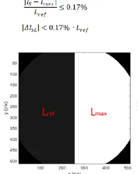
The stray-light correction algorithm performance requirement for 3MI is defined relative to an extended scene consisting of one part of the field of view illuminated at a level labelled Lmax and the other side at a level Lref ≈0.1∙Lmax. Figure 2
shows the nominal signal for an extended scene with the transition between Lmax and Lref at the center, however the
transition could be located at any position and orientation inside the field. The illustration also emphasizes the vignetted areas in the corners of the detector, which come from the fact that the instrument field of view is smaller than the detector array. If IS represents the nominal signal, free of stray-light, and Icorr is the signal numerically corrected from
stray-light, then the stray-light correction performance requirement is given by equation (1) below. This requirement should be fulfilled on pixels located at a distance larger than 5 pixels from the transition between Lmax and Lref. The
requirement translates as a maximum residual stray-light ΔISL allowed after post-processing (equation (2)). With an
initial stray-light of 3%∙Lmax, the performance target corresponds to a stray-light reduction by a factor of about 176.
(1) (2)
Figure 2. Nominal signal for an extended scene with half of the scene at Lmax radiance level and half of it at Lref radiance
level (illustration on the VNIR camera).
In this paper, the stray-light correction principle is described as well as its performances for the VNIR camera. The algorithm is based on the prior on-ground calibration of the stray-light as a function of the field of view. The on-ground calibration method is described, as well as the consequences of inaccuracies during the calibration process.
2. STRAY-LIGHT CORRECTION PRINCIPLE
2.1 Algorithm principle and performance
To understand the stray-light correction principle, it is necessary to introduce the concept of Spatial Point Source Transmittance (SPST) map. An SPST map corresponds to the stray-light profile at detector level assuming a punctual field (point source) illumination of the instrument (i.e. collimated beam for instruments like 3MI with object at infinity). Moreover, the SPST is normalized with respect to the nominal signal at detector level. If (i,j) is the subscript of a pixel on the detector, SPSTi,j is the SPST map associated to the field of view position which hits nominally and with a signal
equal to 1 the pixel (i,j), i being the row and j the column numbers. Given an input scene which gives a nominal signal Inom at detector level, the total signal obtained is the nominal one superimposed to the stray-light signal. As equation (3)
below shows, the total stray-light signal is the result of the linear combination of the SPST maps associated to pixel (i,j) by the nominal signal at that pixel.
(3) This equation (3) can be written in a matrix form (equations (4) and (5)), where a signal at detector level is reshaped from a matrix to a vector. By building matrix ASL where each column contains the SPST maps reshaped as vector, the
stray-light map ISL is obtained by multiplying ASL by the vector-shaped Inom.
(4) (5) An iterative approach was used to get the image corrected from stray-light, which can be implemented with the set of equations (6) to (8) below. The principle is that it is possible to get an estimation of the stray-light signal by calculating the matrix product of ASL by the measured signal Imes. The estimated stray-light is slightly overestimated as the
modulation is made by a signal which is larger than the nominal signal. The residual error can be decreased by modulating the ASL matrix by the measured signal to which the estimated stray-light is subtracted. By performing this
operation iteratively, the residual stray-light error converges toward zero in the way of a dump harmonic oscillator. (6) (7) (8) To evaluate the converging method performance, the algorithm was tested on the ray-tracing optical model of the VNIR instrument. The SPST maps associated to each pixel inside the instrument field of view were computed by ray-tracing. The stray-light pattern for an extended scene was then calculated by modulation of the SPST maps by their associated nominal signal. Then, the correction algorithm was applied to the total extended scene signal, containing both the nominal and stray-light signals. At first iteration, the maps are modulated by the total signal while at the next iterations the maps are modulated by the estimated corrected signal. At each iteration, the estimated stray-light was compared with the real stray-light pattern and the statistical error at 2 sigma was computed. It was expected that the convergence would be affected by the initial level of stray-light. Thus to investigate this effect the exercise was performed by applying different scale factors to the SPST maps (1/5; 1; 5; 10). Figure 3 below shows the residual stray-light error as a function of the iteration number for the different initial levels of stray-light. For the real level of stray-light of 3MI, the residual error is below 10-4∙L
max=10-2∙Lref and thus the required stray-light correction by a factor of about 176 is already reached
with 1 iteration. However, in practice 2 iterations are performed to take some margin, giving a stray-light residual error 2 orders of magnitude lower.
Figure 3. Residual stray-light error of the stray-light correction algorithm as a function of the iteration number (curves normalized to Lmax).
From the results of figure 3, it can be deduced that the residual error increases quadratically with the initial stray-light level. Furthermore, the convergence speed increases when the initial stray-light level decreases. Provided a few approximations, a mathematical model can be derived to predict the residual error as a function of the iteration number (equation (9)). As shown in equation (9), the residual error evolves as a power law of average stray-light level multiplied by the total number of pixels (N×N=512×512 for the VNIR detector). When compared to simulation results, this mathematical model provides an excellent fit and represents thus an efficient way of predicting the convergence behavior based on knowledge of the average stray-light level.
(9) Zong et al. [6] proposed another way to recover the stray-light free signal, Inom, by a matrix inversion method which can
be derived from equations (4) and (5). The iterative method was selected over the matrix inversion method for several reasons. The intrinsic error of the iterative method is already slightly below requirement at first iteration, and 2 orders of magnitude below at second iteration. It doesn’t require calculating the inversion of a matrix, an operation which can be above the computer capabilities (and required computation time) in the case where ASL is large. For example, the full
resolution ASL matrix of the VNIR instrument has 512²×512² elements, which means 67 billion elements! Also, a method
involving matrix inversion is subject to error amplification. Furthermore, the iterative method allows a non-square dimension for ASL, which means that the binning scheme in the spatial and field domains does not necessarily need to be
identical.
2.2 Impact of errors in ASL
In practice, the SPST maps are affected by errors leading to an error dA on the ASL matrix (equation 10). These errors
can come from multiple sources, for example the acquisition noise during the calibration of the SPST maps or even the binning of the maps. It can be shown that such errors doesn’t affect the convergence speed or the residual stray-light at first iteration. However, errors on ASL will limit the convergence to dS, which is equal to the modulation of dA by the
nominal scene (equation 11).
- (10)
- (11)
It can be assumed that all elements in matrix dA are random variables with gaussian distribution and centered on 0. Hence, the residual error of each elements of dS is random variable with gaussian distribution and centered on 0 (equation 12). The standard deviation of dS at each pixel is equal to the modulated root squared sum (RSS) of the standard deviation of elements of dA (equation 13).
- (12)
- (13)
A simple case to derive is when the error dA has the same property on each pixel, which means that std[dA(m,k)]=δ can be written. In that case, equation 13 can be simplified and it is possible to derive a specification on δ from the stray-light correction performance requirement. Indeed, in that case the term δ simply multiplies the root squared sum of the nominal signal at pixel k. Equation 14 below shows the requirement on δ for an extended scene with a transition between Lmax and Lref at the center of the detector. In that equation, the number 333.78 comes from the root squared sum of the
nominal signal. The transition could possibly be located at any position/orientation and the requirement will be the most stringent when a larger part of the detector is illuminated at Lmax. Consequently, a worst case to the requirement would be
when the full scene is at Lmax as given in equation (15). Because δ is a standard deviation, these requirements are to be
understood at 1 sigma. A factor 1/2 and 1/3 must be considered to fulfill the performance requirement at 2 and 3 sigma respectively. These numbers are very useful to write the error budget and perform the dimensioning of the test setup.
Extended scene (Lmax/Lref) (14)
Uniform scene (Lmax) - (15)
2.3 Stray-light correction with interpolated maps
The 3MI VNIR camera’s detector contains 512×512 pixels. Obviously, it is not possible within reasonable time frame to calibrate the SPSTs associated to each and every pixels. Consequently, the calibration is performed on a field of view grid which is less dense than the detector array. Hence, when the ASL matrix is built with these maps, the nominal signal
Inom which is used to modulate ASL must be binned spatially to the same grid as the calibration grid. This leads to two
effects: first the spatial frequencies of the nominal scene are smoothened, second it assumes that the stray-light property doesn’t vary for fields within binned area, which is of course a very strong approximation. This would lead to errors on the estimated stray-light, for 3MI in particular where 27×27 maps are calibrated this would lead to a very poor correction performance.
The proposed solution is to increase artificially the number of SPST maps by interpolation. Several methods were tested, from optical flux interpolation to interpolation in the field domain. Finally, the selected approach is based on an assumption of local symmetry of the stray-light property and is implemented by applying a combination of rotation and scaling of the neighboring SPST maps. Because the local symmetry assumption is valid especially far from the center of the detector, the calibration grid close to the center was doubled. Figure 4-left shows the calibration grid, it consists of 735 fields, regularly spaced with a density doubled at the center.
The interpolation method was implemented and tested with SPST maps obtained by ray-tracing in the 3MI optical model. SPST maps were traced for field points belonging to the calibration grid as well as at intermediate field positions. The idea was to apply the interpolation method to the maps on the calibration grid and compare the result with real SPST maps at intermediate/in-between fields. The target was to obtain interpolated SPST maps close enough to the real SPST maps such that the statistical error is below the value required by equation 15. Once the interpolation method was optimized, it was tested with the full stray-light correction algorithm applied on an extended scene. The blue curve on figure 4-right shows a profile of the stray-light as estimated with the interpolated stray-light maps, considering an extended scene with the transition at the center of detector. ASL was indeed constructed with full spatial resolution SPST
stray-light to which the requirement is both added and subtracted. The stray-stray-light correction algorithm reaches the target performance if the blue curve remains within the 2 red curves. This exercise was also done for extended scenes with transitions located at different positions. Table 1 gives the statistical residual error after stray-light correction for the different scenes considered. As shown in table 1, the residual stray-light is below the required value for all cases except when the transition is at x=128pix where it is very slightly above. This latter result can be explained by the fact that the detector is filled with a larger quantity of signal at Lmax, thus yielding a larger initial absolute level of stray-light.
Figure 4. (Left) Field of view calibration grid for the SPST maps in the 3MI VNIR camera. (Right) Profile of the stray-light (normalized to Lmax) in the 3MI VNIR instrument for an extended scene with transition at center of the detector. The blue
curve corresponds to the estimated stray-light obtained with interpolated SPST maps, the red curves correspond to the frontier in which the blue curve should stay for the algorithm performance to reach its target.
Table 1. Residual error on the estimated stray-light with interpolated SPST maps, considering an extended scene with transition between Lmax and Lref at different positions on the detector.
Transition position
Residual stray-light
1 sigma 2 sigma
x=385 pix 0.024 %∙ Lref 0.060% ∙ Lref
x=256 pix 0.061 %∙ Lref 0.148 %∙ Lref
3. CALIBRATION
3.1 SPST maps calibration
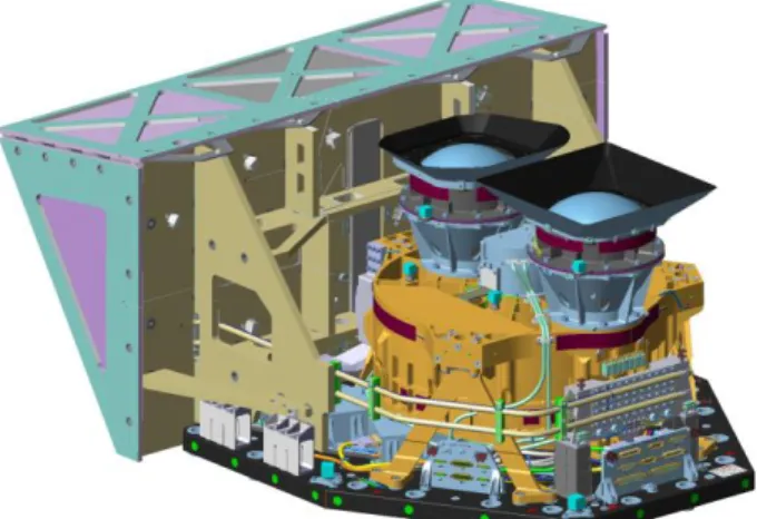
The calibration of the SPST maps is to be performed in CSL’s clean room, under thermal operation conditions inside a vacuum chamber. The Optical Ground Support Equipment (OGSE) consists of a collimator, whose position and orientation relative to the instrument is varied with a mechanical positioner to illuminate the instrument at different fields. The collimator consists of an off-axis parabola, illuminated with a fiber fed with white light. A pinhole limits the extent of the source so that the beam has an angular extent smaller than one pixel at instrument level. Because the source is polychromatic, the SPST maps can be calibrated for all the channels while rotating the filter wheel. This is indeed necessary as the stray-light properties vary with the wavelength, both in geometry and in intensity. Hence, the ASL matrix
in the correction algorithm depends also on the wavelength.
To ensure that the each SPST map acquired contains the stray-light of the instrument only, a set of baffles are used to limit the stray-light generated by the OGSE and test facility themselves (figure 5). The stray-light analysis of the OGSE has shown a rejection ratio by more than 4 orders of magnitude around the direction of the beam. The stray-light drops very fast to reach 10 orders of magnitude rejection at only 10 degrees the beam. Consequently, the contribution of the OGSE stray-light in the acquired SPST will be negligible.
Figure 5. (Left) SPST maps calibration optical ground support equipment. (Right) Stray-light from the OGSE
With a square aperture of 38 mm, the collimated beam is large enough to illuminate the entrance pupil of 3MI but is too small to cover the full 170 mm first lens of the instrument. However, if most of the stray-light of the instrument is generated after the aperture stop, some stray-light will occur before that element in the camera. Hence, it is necessary to illuminate more than the entrance pupil to grasp the full stray-light contributions in the SPST maps. For that, the collimated beam is scanned on the first lens and the different images acquired are recombined to form the full SPST map. With no prior knowledge of the instrument, this means that the scan should cover the full first lens. However, it can be shown that not all areas are generating stray-light at detector level. In that frame, the stray-light entrance pupil has been defined as the area which generates stray-light at detector level, either from ghosts reflections of scattering [7]. In the case of ghost reflections, the main contributor to stray-light in 3MI, it was shown that the stray-light entrance pupil is localized close to the entrance pupil. By performing between 2 and 7 scans the full SPST maps from ghost reflections can be obtained. In the case of scattering due to either roughness or contamination, the stray-light entrance pupil has a larger extent as the scattering occurs on ±90°, however the areas far from the nominal entrance pupil contribute to stray-light levels orders of magnitude lower than the ghost contributions. The stray-stray-light entrance pupil was calculated/defined by simulations and will be used as a baseline/input for the on-ground calibration of the SPST maps. For a few field of view positions, however, the full first lens will be illuminated to verify the validity of the stray-light entrance pupil simulation results. The stray-light entrance pupils obtained by simulation were used to estimate the error contribution due to inaccuracies in the scan of the OGSE, it was shown that the contribution was much smaller than required by equation 15 [7].
The noise at detector level is a very critical parameter to be taken into account as it affects significantly the accuracy of the SPST maps on-ground calibration. For the VNIR camera, the detector has 14 bits, which means that variations of the stray-light below (214-1)-1 =6.1∙10-5 cannot be measured. In addition, the signal at detector level is submitted to a noise
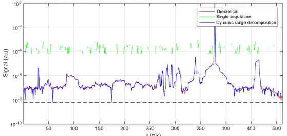
whose standard deviation is given by equation (16) below. In that equation, I is the nominal signal received by the detector, a=3 is the read-out noise and b=0.01333 is a parameter intrinsic to the detector (VNIR). Consequently, if a SPST map is acquired in a single acquisition with the nominal signal slightly below the saturation of the detector, the details in the SPST maps are completely lost. The solution to this problem is to acquire SPST maps by decomposing the dynamic range. For that, three acquisitions are performed with different input flux levels. The different images are recombined bottom-up. For the image acquired with the highest flux, only the signal which is below 0.9 times the saturation is kept. For the second acquisition, the values kept are those which are 0.9 times the saturation and which were not already kept in the first acquisition. The same principle applies for the first iteration and finally the three images are recombined with a normalization factor corresponding to the ratio of the input flux.
- (16)
Figure 6 below shows an example of the map acquired with the dynamic range decomposition. The green curve corresponds to the result of a single dynamic range acquisition and demonstrates the need of doing such decomposition. The blue curve corresponds to the recombination of images acquired on three different dynamic ranges and shows excellent correspondence with the red curve which represents the theoretical curve.
Figure 6. Example of SPST map acquisition result with either a single acquisition or the dynamic range decomposition.
The performance of the stray-light correction algorithm was verified considering the SNR on the detector as obtained with the dynamic range decomposition. For that the ray-tracing SPST maps on the calibration grid were considered and interpolated on the 256×256 field of view grid. The noise model together with the dynamic range decomposition principle was applied to each SPST map. Finally, the estimated stray-light with such maps was compared with the real stray-light, deriving the statistical residual stray-light error. Table 2 below shows the results, considering extended scenes with transition between Lmax and Lref at different positions on the detector. As shown in table 2, the stray-light correction
performance is slightly decreased compared to the case without SNR which was shown in table 1. If the performance at 2 sigma for the case of a transition at x=128 pixel is slightly above the requirement, in all other cases the residual stray-light remains below the required value.
Table 2. Residual error on the estimated stray-light with interpolated SPST maps, considering an extended scene with transition between Lmax and Lref at different positions on the detector. The noise at detector is considered and a the
dynamic range is subdivided in 3 Transition
position
Residual stray-light
1 sigma 2 sigma
x=385 pix 0.029 %∙ Lref 0.063% ∙ Lref
x=256 pix 0.067 %∙ Lref 0.156 %∙ Lref
x=128 pix 0.086 %∙ Lref 0.189 %∙ Lref
4. CONCLUSION
A stray-light correction algorithm was implemented for the 3MI instrument with the goal to reduce the stray-light from its initial level of about 3%∙Lmax down to 0.17%∙Lref, considering as a reference for performance evaluation an extended
scene with a transition between Lmax spatially uniform radiance level and Lref≈0.1∙Lmax. The correction method principle
is based on the calibration of spatial point source transmittance maps, which corresponds to the stray-light pattern associated to a punctual illumination of the instrument. The estimated stray-light associated to the scene is first estimated by modulating the SPST maps by the measured scene. The residual stray-light error is then reduced iteratively by modulating the maps by the estimated corrected signal. It was shown that 1 iteration was already enough to fulfill the instrument requirement, 2 iterations were however selected to take some margin. The stray-light algorithm performance was discussed and exercised with ray-traced SPST maps from the 3MI optical model, implemented in the FRED software. Moreover, the accuracy requirements for the SPST maps calibration was presented. The calibration test setup consists of a collimated beam which illuminates the instrument. Baffles are used to avoid recording the stray-light contribution of the test setup itself. Scan of the first lens is performed to acquire the different stray-light contributors of 3MI, and dynamic range decomposition is performed to obtain a high signal to noise ratio. Because it is not possible to calibrate the SPST maps associated to each pixel of the detector, an interpolation method was implemented to increase artificially the number of available maps. The performance of the algorithm was verified with ray-tracing data, considering the detector noise with dynamic range decomposition. When considering an extended scene with the transition at the center, the residual stray-light level is below the maximum level required by the end users.
REFERENCES
[1] Manolis, I., Caron, J., Grabarnik, S., Bézy, J-L., Betto, M., Barré, H., Mason, G., Meynart, R., "The MetOp Second Generation 3MI mission", Proc. SPIE 10564, International Conference on Space Optics — ICSO 2012, 105640A (20 November 2017)
[2] Manolis, I., Bézy, J.-L., Meynart, R., Porciani, M., Loiselet, M., Mason, G., Labate, D., Bruno, U., De Vidi, R., "The 3MI instrument on the MetOp Second Generation", Proc. SPIE 10563, International Conference on Space Optics — ICSO 2014, 1056324 (17 November 2017)
[3] Bruno, U., Mastrandrea, C., Mosciarello, P., Gabrieli, R., Boldrini, F., Porciani, M., Langevin, M-N., “3MI: multi-viewing, multi-channel, multi-polarization imaging for METOp second generation”, Proc. International Astronoautical Congress, IAC-17-B1.3 (25-29 September 2017)
[4] Laherrere, J-M., Poutier, L., Bret-Dibat, T., Hagolle, O., Baque, C., Moyer, P., Verges, E., "POLDER on-ground stray light analysis, calibration, and correction", Proc. SPIE 3221, Sensors, Systems, and Next-Generation Satellites, (31 December 1997)
[5] Fest, E., "Stray Light Analysis and Control", SPIE press, March 2013
[6] Zong, Y. Brown, S., Meister, G., Barnes, R., Lykke, K., "Characterization and correction of stray light in optical instruments", Proc. SPIE 6744, Sensors, Systems, and Next-Generation Satellites XI, 67441L (26 October 2007)
[7] Clermont, L., Michel, C., Mazy, E., Pachot, C., Stockman, Y. “Stray-light characterization and correction in the MetOp-SG 3MI instrument”, CNES Stray-light Workshop, Toulouse, 15th November 2017