HAL Id: halshs-00193374
https://halshs.archives-ouvertes.fr/halshs-00193374
Submitted on 3 Dec 2007
HAL is a multi-disciplinary open access archive for the deposit and dissemination of sci-entific research documents, whether they are pub-lished or not. The documents may come from teaching and research institutions in France or
L’archive ouverte pluridisciplinaire HAL, est destinée au dépôt et à la diffusion de documents scientifiques de niveau recherche, publiés ou non, émanant des établissements d’enseignement et de recherche français ou étrangers, des laboratoires
If only I could borrow more! Production and
consumption credit constraints in the Philippines
Marie Godquin, Manohar Sharma
To cite this version:
Marie Godquin, Manohar Sharma. If only I could borrow more! Production and consumption credit constraints in the Philippines. 2005. �halshs-00193374�
Maison des Sciences Économiques, 106-112 boulevard de L'Hôpital, 75647 Paris Cedex 13
http://mse.univ-paris1.fr/Publicat.htm
If only I could borrow more ! Production and consumption credit constraints in the Philippines
Marie GODQUIN, TEAM Manohar SHARMA, TEAM
If only I could borrow more!
Production and consumption credit constraints in the Philippines.
Marie Godquin
∗and Manohar Sharma
∗∗Fist draft: September 2004 This version: January 2005
∗ TEAM (University of Paris I – La Sorbonne) and CNRS, 106-112, Bd. de l’Hôpital, 75013 Paris,
marie.godquin@univ-paris1.fr
This paper provides a new approach to analyzing credit constraints by differentiating which of the household’s production and consumption decisions are affected by credit constraints. It also provides a first attempt to estimate of the extent and determinants of credit constraints in the Philippines. Based on direct questions on households’ experiences in credit markets, we estimate the percentage of credit-constrained households at 65%. The lack of credit constrained the level of agricultural production of 37% of the farming households; it also constrained the level of family business production of 31% of the households operating such businesses. Credit constraints also limited consumption choices of 21% of the sample households. We found that the presence of credit programs operating in the village and proximity to commercial banks and rural banks reduced the probability of credit constraints in production decisions. Further, some types of households are more likely to experience credit constraints. These are the households with little education, households that own little or no titled land, and sugar-producing households.
Keywords: Credit constraints, Philippines, Asia.
Ce papier propose une nouvelle approche des problèmes de contraintes de crédit en ce qu’il différencie quelles décisions de production ou de consommation du ménage sont affectées par les contraintes de crédit. Ce papier constitue également la première analyse de l’étendue et des déterminants des contraintes de crédit aux Philippines. A l’aide de questions sur l’expérience des ménages sur le marché du crédit, nous estimons le pourcentage de ménages contraints à 65%. Le manque de crédit contraignait ainsi les choix productifs agricoles de 37% des ménages agricoles de même qu’il contraignait 31% des choix productifs des ménages opérant une activité non agricole. Les contraintes de crédit affectaient également les choix de consommation de 21% des ménages enquêtés. Certains ménages sont plus exposés aux contraintes de crédit. Ce sont les ménages ayant un faible niveau de capital humain, les ménages possédant peu de terres avec titre de propriété et les ménages producteurs de canne à sucre. La présence de programmes de crédit opérant dans le village de même que la proximité de banques rurales ou commerciale permet de réduire les contraintes de crédit, tout du moins dans le domaine productif.
Mots clefs : Contraintes de crédit, Philippines, Asie. JEL codes: O12, O16
1. Introduction
The Philippine rural financial sector has undergone dramatic changes in the past quarter century. It has evolved from a supply-led finance approach in the 1970s and 1980s characterized by loan targeting, credit subsidies and directed loans to certain sectors, to market-oriented financial and credit policy. Interest rate caps were lifted in the
early 1980s, government banks and rural banks1 were restructured in 1986-1987, bank
entry and branching was liberalized in the early 1990s, the Central Bank was restructured in 1993, foreign banks were allowed to enter the market in 1994, and the country’s largest bank, the Philippine National Bank, was privatized. However, the government was still heavily engaged in highly subsidized directed credit programs (DCPs) in the 1990s with 21 government agencies implementing 86 such programs (Llanto, Geron and Tang, 1999). As detailed in Llanto (2001), the Filipino rural financial sector in the 1990s was characterized by the huge fiscal cost of unsustainable DCPs and low financial discipline among borrowers, a weakened rural banking system dependent on subsidized funds, and inefficient targeting. This situation led the government to phase out all DCPs
by 2002 for both the agriculture sector and the non-agricultural sector2 and adopt a
demand-driven approach to rural finance.3 Aside from providing financing opportunities,
access to credit indeed stimulates productive investments and reduces the risk-vulnerability of rural households that might be therefore more willing to adopt new technologies (Eswaran and Kotwal, 1990). The Medium-Term Philippine Development Plan (MTPDP) for 2001-2004 recognizes the importance of an efficient, sustainable and demand-driven rural financial market and emphasizes the importance of increasing access to credit, including long term financing of small farmers and indigenous peoples and promoting a savings-led approach to agricultural and small off farm business financing.
1 Between 1980 and 1987, the total volume of loans from formal institutions declined by 44% in real terms;
three commercial banks, 147 rural banks and 32 thrift institutions failed (Cho and Khatkhate, 1990).
2 The Agriculture and Fisheries Modernization Act (AFMA) passed in 1997 is the legal basis for the
withdrawal of the government from agricultural DCPs. Its equivalent for the nonagricultural sector is Executive Order 138, passed in 1999.
3 The Agricultural Modernization Credit and Financing Program (AMCFP) of 1997 specifies that all
lending decisions and credit delivery should be made through banks and strong or viable cooperatives and NGOs, excluding the government or non-government non-financial institutions from that field.
How credit constrained are rural households after financial liberalization? Previous studies on rural financial markets in the Philippines have described its policy environment (e.g. Esguerra, 1996 and Adams, Chen and Lamberte, 1993), the nature of interlinkages with the credit market (Floro and Yotopopulos, 1991 and Nagarajan, David and Meyer, 1992), the demand for agricultural loans (Nagarajan, Meyer and Hushak, 1998) and the role of credit market in mitigating shocks (Fafchamps and Lund, 2003; Fafchamps and Gubert, 2002). Empirical studies on access to credit and credit constraints are still lacking for the Philippine rural sector.
Thus, this paper aims to provide information on the extent of credit rationing and its determinants in the rural Philippines. We develop a method of elicitation of credit constraints based on the approach of Feder, Lau, Lin and Luo (1990) that allows us to differentiate which of the household’s decisions on consumption and agricultural and off-farm production are affected by credit constraints. We use this information to develop models of the joint probability of being constrained across multiple activities, including agricultural production, a non-farm family business and consumption.
The remainder of the paper is organized as follows: section 3 reviews approaches that have been used in the literature to measure households’ access to credit and credit constraints. Section 3 develops our empirical model and section 4 describes the setting, sample and survey instruments. Section 5 presents the results of the empirical model while the final section concludes and discusses some policy implications.
2. Identification of credit constraints in the literature
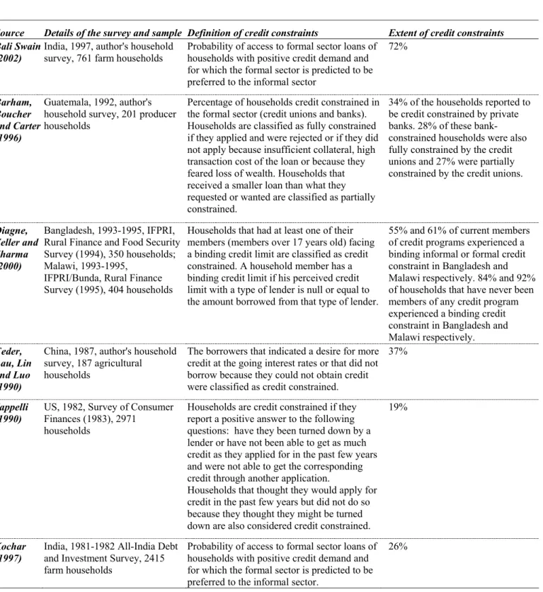
Previous studies have found that the percentage of credit constrained households ranges from 19% to 72% as shown in Table 1. However, it is difficult to compare these estimates given the differences in the study samples and the methodologies used for eliciting credit-constrained status. The following of this section will thus review the different approaches to measure credit constraints.
Table 1 Prevalence of credit rationing
Source Details of the survey and sample Definition of credit constraints Extent of credit constraints Bali Swain
(2002)
India, 1997, author's household survey, 761 farm households
Probability of access to formal sector loans of households with positive credit demand and for which the formal sector is predicted to be preferred to the informal sector
72% Barham, Boucher and Carter (1996) Guatemala, 1992, author's household survey, 201 producer households
Percentage of households credit constrained in the formal sector (credit unions and banks). Households are classified as fully constrained if they applied and were rejected or if they did not apply because insufficient collateral, high transaction cost of the loan or because they feared loss of wealth. Households that received a smaller loan than what they requested or wanted are classified as partially constrained.
34% of the households reported to be credit constrained by private banks. 28% of these bank-constrained households were also fully constrained by the credit unions and 27% were partially constrained by the credit unions.
Diagne, Zeller and Sharma (2000)
Bangladesh, 1993-1995, IFPRI, Rural Finance and Food Security Survey (1994), 350 households; Malawi, 1993-1995,
IFPRI/Bunda, Rural Finance Survey (1995), 404 households
Households that had at least one of their members (members over 17 years old) facing a binding credit limit are classified as credit constrained. A household member has a binding credit limit if his perceived credit limit with a type of lender is null or equal to the amount borrowed from that type of lender.
55% and 61% of current members of credit programs experienced a binding informal or formal credit constraint in Bangladesh and Malawi respectively. 84% and 92% of households that have never been members of any credit program experienced a binding credit constraint in Bangladesh and Malawi respectively.
Feder, Lau, Lin and Luo (1990)
China, 1987, author's household survey, 187 agricultural households
The borrowers that indicated a desire for more credit at the going interest rates or that did not borrow because they could not obtain credit were classified as credit constrained.
37%
Jappelli (1990)
US, 1982, Survey of Consumer Finances (1983), 2971
households
Households are credit constrained if they report a positive answer to the following questions: have they been turned down by a lender or have not been able to get as much credit as they applied for in the past few years and were not able to get the corresponding credit through another application.
Households that thought they would apply for credit in the past few years but did not do so because they thought they might be turned down are also considered credit constrained.
19%
Kochar (1997)
India, 1981-1982 All-India Debt and Investment Survey, 2415 farm households
Probability of access to formal sector loans of households with positive credit demand and for which the formal sector is predicted to be preferred to the informal sector.
There are three main approaches to measuring credit constraints in the literature. The first type is an indirect method that infers the presence of credit constraints based on predictions from theory, such as the violation of the permanent income hypothesis, a difference between the shadow price of capital and the cost of credit, or changes in production activities in response to a change in eligibility status to formal credit. The second type of methodology is a semi-direct method as it uses access to the credit market to identify credit constraints. The third approach uses direct questioning of households or production units on their realized and latent credit experiences. We detail in the following these approaches and their most influential papers.
2.1. Indirect methods of eliciting credit constraint
One of the testable implications of the permanent income/ consumption-smoothing hypothesis is that in the absence of liquidity constraints, consumption changes are correlated with significant changes in lagged earnings or predicted changes in earning but not with transitory income shocks (Hall, 1978; Deaton, 1992). Various studies have thus used the rejection of the permanent income hypothesis as a test for the existence of liquidity constraints. Zeldes (1989) is one of the most influential of these studies, which used an a priori classification of liquidity constraint. Zeldes divides his sample based on whether the household holds at least two months of income as assets. His test relies on the fact that, if the ratio of wealth and financial assets to disposable income is a good indicator of liquidity constraints, the permanent income hypothesis is likely to be verified for households with high assets and rejected for low-wealth households. Indeed, Zeldes finds that lagged income is only significant for the low asset group.4 Several other papers
have tested the permanent income hypothesis but no consensus has been reached on whether there is excess sensitivity of consumption to transitory income shocks that would be attributed to credit constraints (see Browning and Lusardi (1996) and Besley (1995) for a review). Moreover, Browning and Lusardi (p1832-1833) list several empirical and theoretical reasons that might lead to the rejection of the permanent income hypothesis
4 Jappelli (1990) however shows that the use of exogenous and fixed ratios is inappropriate to proxy
liquidity constraints because it leads to the inclusion of unconstrained households in the low-wealth group and constrained households in the high-wealth group (see Jappelli, 1990, p. 232-233 for a numerical example).
even in the absence of liquidity constraints. Carroll (1992), for example, explains the rejection of the permanent income hypothesis due to precautionary savings behavior.
Sial and Carter (1996) used another type of indirect method to test for credit constraints. They estimate the shadow price of credit for small Pakistani farmers and find a large gap between the shadow price and the prevailing formal market loan rates. They attribute this large gap (around 190% for non borrowing farmers and around 60% at the mean loan size) to credit constraints faced by the farmers. However, this approach requires detailed information on revenues, cost and technology and is difficult to implement when there is heterogeneity of production activity and technologies both within and across households. Moreover, as explained earlier, other element of the credit contract such as collateral requirement or repayment schedules might generate a substantial difference between the nominal interest rate and the total credit cost.
Banerjee and Duflo (2002) provide a new approach to determine whether firms are credit rationed based on firms’ reaction to a change in eligibility of directed lending programs. Both constrained and unconstrained firms are likely to be willing to borrow more from the formal sector if it is cheaper than other credit sources. If the increase in formal borrowing does not translate to production growth, the authors argue that firms are unconstrained and use the additional credit as a substitute for other borrowing. Credit constrained firms on the contrary will use it to expand their production. While this approach provides an interesting test of credit rationing it is applicable only in a context where a policy change in the supply of credit can be clearly identified. Furthermore, translating this approach to rural households might be problematic if credit is fungible and the increase in formal credit does not translate to an increase in agricultural or non-agricultural production but an increase in asset accumulation or consumption expenditures.
2.2. Approaches based on realized credit transactions
A second class of methods uses observable market outcomes to elicit credit rationing. Earlier studies have proxied credit rationing by the absence or non-use of formal loans. However, this is likely to be a crude approximation since, as previously shown, there is no simple relationship between credit rationing or credit constraints and
borrowing. Borrowing households could be willing to borrow more without having access to additional credit. Other households may also choose not to borrow because they are risk averse. In addition, these studies often assume that borrowing from the formal credit market is always preferable to borrowing from the informal credit market given the high value of local moneylenders’ interest rates.
Kochar (1991, 1997) presents a model of access to credit that relaxes these assumptions. Using estimates of the informal and formal marginal interest rate for both borrowers and non-borrowers, she is able to determine whether the formal sector should
be preferred to the informal sector.5 Unfortunately Kochar cannot distinguish between
constrained and unconstrained non-borrowing households and assumes that non-applicant households have no demand for credit. This prevents us from classifying as credit constraints discouraged borrowers that did not apply because they thought they would be denied or because they were too far from a lender. While Kochar mentions that borrowers that borrow from both the formal and the informal sector are likely to be quantity constrained by the formal sector, this is not taken into account in the analysis that focuses on access and only indirectly on credit rationing. Bali Swain (2002) uses Kochar’s model and adjusts its empirical specification using information on rejection of loan applications. As the author recognizes, the empirical specification still lacks information on quantity credit constraints and discouraged borrowers, which does not allow her to provide a complete picture of credit constrained borrowers.
2.3. Direct elicitation of credit constraints
Three types of direct questions have been used to elicit credit constraints based on household’s experiences of rejection and need for credit. The first approach first applied by Jappelli (1990), and followed by Zeller (1994), classifies households as credit constrained if they report any rejected application of credit or report being granted less than the amount they initially asked for and were not able to get the corresponding amount through another credit application. Households that did not apply because they thought they would have been turned down are also classified as credit constrained.
5 The preference of the formal sector is also likely to depend on other elements of the loan contract such
Diagne, Zeller and Sharma (2000) asked all adult households members their perceived credit limit with different types of lenders and classify the households as credit constrained if at least one of its members has reached this credit limit. This approach still lacks information on excess demand and relies on the hypothesis that the household members that have reached their credit limit with a certain type of lender would have liked to borrow more from that lender and thus can be classified a credit constrained. It is also unclear why credit constraints of individual household members can easily translate to household level binding credit limit.
The strength of the type of questions used by Feder, Lau, Lin and Luo (1990) is that they rely on no assumptions and directly ask borrowing households whether they would have liked more institutional credit at the going rates of interest. Non-borrowing households were also asked the reason for not borrowing. Borrowing households, which would have liked more institutional credit and non-borrowing households, which reported that they did not borrow because they could not obtain credit, were classified as credit constrained. This approach has been subsequently used by Braham, Boucher and Carter (1996). It relies on the ability of the respondent to perceive credit constraints and report them, but the perception of the households on their credit experience is also more likely to have a more significant impact on their behavior than their ‘true’ credit constraint status. The type of classification by Feder, Lau, Lin and Luo is the one that we will follow in this paper as it relaxes all assumptions on credit constraints and is the one that fits best our definition of credit constraints in terms of unsatisfied positive marginal demand for credit.
2.4. Findings of the empirical literature on the determinants of credit constraints
From the above-mentioned literature, only the papers by Jappelli (1990) and by Feder, Lau, Lin and Luo (1990) and Zeller (1994) have proceeded to an estimation of the determinants of credit constraints. The three empirical models estimate a reduced form of credit constraints since both demand (how much the household would like to borrow) and supply (how much the financial intermediaries are willing to lend to that household) affect credit constraints. All three studies differ in terms of samples and estimation methods. Japelli’s (1990) study is on American households; Feder et al. (1990) is based
on a survey of Chinese farm households (see table 1), and Zeller (1994) on individual household members from Madagascar. Moreover, the determinants of credit constraints analyzed and their impact are not directly comparable. The study by Feder and al. and the study by Japelli show that savings, income and wealth have a negative impact on credit rationning whereas the number of adults in the households and the family size has a positive impact on credit rationing. In the study by Japelli, other demographic variables such as age, marital status and race reduce the probability of being credit constrained6.
These studies identify savings and income as significant determinants of credit constraint status but these variables are also subject to endogeneity bias. Exogenous measures of income and wealth should thus be preferred.
3. The empirical model
Our empirical model is based on an agricultural household model from which we derive
the demand for funds of the household.7 Most of our sample households (72.5%) have
some productive activity: 44% of them are engaged in farming only, 10% are engaged in agricultural activities only and another 18.5% are engaged in both farming and non-agricultural activities. We thus allow for two productive activities in our model. We assume that household members pool their resources and that decisions on expenditures on production and consumption are taken at the household level. In this model, credit constraints are thus defined at the household level and not at the individual level. Our estimations are based on reduced forms of credit rationing.
Every household maximizes a utility function subject to a budget and a time constraint. For simplicity of exposition, we will present a simple two period model where the household maximizes the utility that it derives from its consumption of undifferentiated goods C and of leisure L:
) , , , ( 1 2 1 2 2 1 2 1 L L C C U
Max
L L C C (1)6 Other variables used in the estimation but with no impact on credit rationing include for the study by
Feder et al.: land, capital, number of dependents, education, farm experience, total initial liquid assets, outstanding debt in financial institutions, total outstanding debt and previous loan default and for the study by Japelli: debt, education, unemployment and sex.
where the time subscript 1 refers to the recall period of the survey and the time subscript 2 refers to the “future” period and is meant to capture the duration of the relevant repayment period. The maximization of this function is subject to a budget and time constraint for each of the two periods:8
b a b b b b b a a a a a f K H N p f K H N wM F C I I p1 ( 1, 1, 1)+ 1 ( 1, 1, 1)+ 1 1+ = 1+ + (2a) ) 1 ( ) , , ( ) , , ( 2 2 2 2 2 2 2 2 2 2 2 f K H N p f K H N wM C F r pa λa a a a + b µ b b b b + = + + (2b) 1 1 1 1 H M L H T = a + b + + (2c) 2 2 2 2 H M L H T = a + b + + (2d)
where the subscript a refers to agricultural activity and b to non agricultural businesses, and:
pa, pb: price of agricultural and non agricultural output
Ka1, Kb1: initial endowment of productive capital used for agriculture production and
non-agricultural business, respectively
Ha, Hb: family labor used in the household farm and in the household’s non-agricultural
business, respectively
Na, Nb: on-farm hired labor, hired labor used for the family business.
M: net market labor supply w: market wage rate
F: level of fund requirements C: consumption
Ia, Ib: farm and off-farm business investment and input expenditures such that K2=K1+ϕI
and ϕ is the share of investment expenditures in investment and input expenditures. λ,µ: technical improvement parameter of the farm and non farm sector
r: interest rate or cost of funds T: total household available time L: leisure or non-market time
8 The model of Iqbal (1986) included only the agriculture sector. We have separated hired labor used in
pa and pb should be interpreted as price vectors and fa, fb, vectors of production functions
when the household produces different crops or is engaged in different non-agricultural businesses.
The demand for funds (F) is defined in the previous system as the difference between investment and savings and can be rewritten as:
FA LE B
F = − − 9 (3)
Where the demand for fund (F) is the sum of change in liabilities (B, borrowing – LE,
lending) and change in internal borrowing (FA, net change in financial assets).
We define credit constraints as the situation where the household cannot avail the credit it desires at the prevailing relevant market conditions. The prevailing relevant market conditions, Pm, are in this case defined by the expected rates of interest (r) in the area
associated to loan sizes (L), repayment schedules (RS) and level of guaranties (G);
Pm={rm, Lm, RSm, Gm}.
A household will thus be credit constrained if:
b a b b b b b a a a a a f K H N p f K H N wM F C I I p * * 1 * 1 1 1 1 1 1 1 1 1 1 ( , , )+ ( , , )+ + < + + (4a) b a b b b b b a a a a a f K H N p f K H N wM B L FA C I I p * * 1 * 1 1 1 1 1 1 1 1 1 1 ( , , )+ ( , , )+ + − − < + + (4b)
or, using simplified notation:
FA LE Y I I C P B B< *( m)= 1*+ a*+ b*− 1+ + (4c)
where Y1, the total income in the first period, equals
1 1 1 1 1 1 1 1 1 1f (K ,H ,N ) p f (K ,H ,N ) wM pa a a a a + b b b b b + * B
B< corresponds to C1<C1* or Ia<Ia* or Ib<Ib* or any combination of these sub
constraints and where B is the credit limit of the household and B* its optimal level of borrowing at the prevailling relevant market conditions. C1*, Ia*, Ib* are respectively the
optimal level of consumption expenditures and farm and off-farm level of investment and input expenditures that would be chosen in the absence of credit constraints.
Equation (4c) shows that two factors determine whether the credit constraint will be binding. The left hand side of the inequality represents the credit taken by the household or the household’s credit limit when the constraint is binding, i. e. how much
9 We did not include the variation of the stock of consumer durables in this equation since rural Filipino
financial intermediaries are willing to lend to the household. The right hand side determines the amount the household would like to borrow.
The life-cycle model does not deliver a closed-form solution for the optimal consumption level C* in the presence of borrowing constraints. Moreover, production and consumption are no longer separable. We follow the assumptions made by Jappelli (1990) for his empirical model for the estimation of consumption credit constraints:10
Assumption 1: The reduced form of C*, Ia*, Ib* can be expressed as C*=αcX + εc,
Ia*=αIaX + εIa, Ib*=αIbX + εIb, where X is a matrix of observable variables such as
household demographic characteristics, age and education of the household head, wealth, production choices and accessibility of lenders.
Assumption 2: The debt ceiling, B, can also be expressed as a function of the same observable variables: B=βX + η.
We can thus provide the following reduced form of equation (4c):
Z FA LE Y X c I I c Ia Ib b a + − − + + + + + − = + < (α α α β) 1 ε ε ε η 0 (5)
The optimal level of consumption and investment of the household as well as its credit limit is unobservable but we can identify the households that were credit constrained based on their answer to the question “During the past 12 months, would you have used more credit if it was available to you?”. Furthermore, since we have asked this question by use, for agricultural production, non-agricultural business and non-food expenditures, we can identify which decision is affected by the credit constraint. We can thus define the following three latent credit constraints equations:
Za*= λaX+µa
Zb*= λbX+µb
Zc*= λcX+µc
where λi are linear combinations of the parameters in (4c) and Za*, Zb*, Zc*, the latent
variables representing respectively the reduction in the level of agricultural (Ia*-Ia)
investment, reduction in the level of non-farm business investment (Ib*-Ib) and reduction
in the consumption level (C1*-C1), attributed to credit constraints.
The corresponding index function for consumtion is the following: Zc=1 if λcX+µc >0
Zc=0 if λcX+µc ≤0
which reads: when Zc=1, the household is credit constrained and its consumption decision
is affected (C1*>C1), otherwise, C1*=C1
The two production index functions are defined similarly with the subscript a for agricultural production and b for non agricultural business.
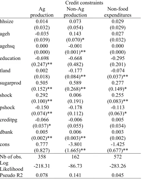
Following the previous discussion, the set of regressors to be used in the estimation of credit constraint will be composed of variables that influence the demand for credit as well as variables that influence the credit limit the household faces. Since we estimate reduced forms, we will not be able to separately identify supply and demand influences on credit constraints. When supply and demand have opposite effects, some variables may not have a significant impact. Furthermore, some variables might have some impact on the demand for funds for production but not for consumption and vice versa. In the following, we discuss the variables we used in our analysis and their impact that we summarize in table 2.
The demand for consumption funds 11 is increasing with the size of the household
but the demand for production funds12 is decreasing with the size of the household as
household labor substitutes for hired labor.
The productive experience of the household increase with the age of the household head and so does the demand for productive funds. We use a quadratic form of the age of the household head to allow for the diminishing impact of age.13 Credit limit should also increase with the productive experience of the household leading to an ambiguous sign of age of the household head.14
11 In the following, we refer to non-food expenditure as consumption to ease the reading. 12 When unspecified, production refers to both agricultural and non-agricultural production.
13 The diminishing impact of age could be explained by a reduction of marginal experience gain with age.
The stock of productive assets also increases with age and could aslo lead to diminishing impact of age on the demand for fund.
14 A diminishing impact of age on credit ceiling could also be explained by reduced marginal experience
gain with age. It could also be explained by higher probabilities of death as age increase if debt is difficult to transfer to children in case of death.
Better-educated households are expected to be better able to exploit investment opportunities when they arise and generate higher incomes in the future. Therefore, the demand for production funds is likely to increase with education of the household head. Education is also supposed to increase the demand for funds for consumption through expectations of a higher income in the future. The same arguments play in the same direction for the assessment of repayment capacity on the demand side, leading to an ambiguous sign. We use the percentage of households members over 14 years old with six or more years of education for the education of the household.
Size of cultivated land increases with the area of titled land and so do farm working capital. On the supply side, titled land can serve as collateral and increase the credit limit of the household. The area of titled land is also a proxy for wealth and is associated with better repayment capacity. Sugar producers have higher working capital requirements as each sugar cane sapling can be used for two to three planting seasons only, while expense in fertilizer and harvesting costs (use of harvesters and transportation costs) are higher. Sugar producers are thus more likely to use more credit for their agricultural production and thus have less external funds available to finance their other needs.
Households often cope with negative shocks by incurring loans or liquidating part of their financial assets. In the aftermath of such a shock, their stock of financial assets available for production and consumption is depleted which translate in a larger demand for external funds to keep the level of production and consumption expenditures constant. On the supply side, the increase in the level of household debt or the decrease in its financial assets (and capacity to cope with future shocks) affects negatively the amount the lenders are willing to lend to the household for production and consumption expenditures. Positive covariant shocks affecting the households increase their investment opportunities and thus their demand for credit.
The last group of variables that we will consider refers to the accessibility of financial intermediaries. The availability of credit services in a village is increasing with the number of government and NGO credit programs and decreasing with the distance to commercial banks. If lenders are constrained in the total amount they can lend or if there is little flexibility in their contractual arrangements, making their financial services de
facto unavailable for some of the households, then the availability of credit services in the village can increase the credit limit of some households.
To limit the extent of endogeneity bias, we did not include direct measures of savings, debt, income and non-food expenditures in our set of regressors as was done in previous studies, even if lenders use them to assess creditworthiness.
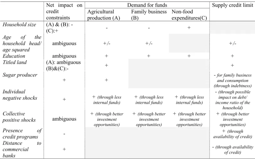
The following table summarizes the expected impact of our regressors on the external optimal demand for funds and credit limit. Variables that have a positive impact on the demand for funds increase the probability that the household is credit constrained whereas variables that have a positive impact on the household credit limit decrease its probability of being credit constrained.
Table 2 Predicted impact of the regressors on demand and supply side of credit constraints
Demand for funds Net impact on
credit
constraints Agricultural production (A)
Family business (B)
Non-food expenditures(C)
Supply credit limit
Household size (A) & (B): -
(C):+ - - + Age of the household head/ age squared ambiguous +/- +/- +/- Education ambiguous + + + +
Titled land (A): ambiguous
(B)&(C):- + +
Sugar producer
+ + - for family business and consumption
(through indebtness)
Individual
negative shocks + + (through less internal funds) + (through less internal funds) + (through less internal funds) - (through possible impact on debt/ income ratio of the
household)
Collective
positive shocks ambiguous
+ (through better investment opportunities) + (through better investment opportunities) + (through better investment opportunities) + (through better investment opportunities) Presence of
credit programs - availability of credit)+ (through
Distance to commercial
banks
+ - (through availability
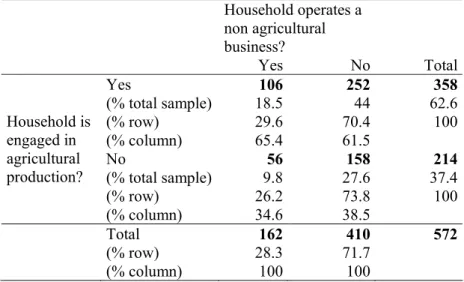
There are alternative candidate econometric strategies to estimate these three index functions. The first one is to estimate the three equations using three independent probits. However we observe the agricultural credit constraint outcome only on the subsample of agricultural producers (62.6%) and we observe the non agricultural credit outcome only on the subsample of households (28.3%) that operate a non agricultural business (table 3). It is possible that the agricultural households don’t share the same characteristics as the non agricultural households resulting in biased coefficients of these two probit models. We thus tested for selection bias for these two equations.
Table 3 Repartition of the sample households based on their production status
Household operates a non agricultural business? Yes No Total Yes 106 252 358 (% total sample) 18.5 44 62.6 (% row) 29.6 70.4 100 (% column) 65.4 61.5 No 56 158 214 (% total sample) 9.8 27.6 37.4 (% row) 26.2 73.8 100 Household is engaged in agricultural production? (% column) 34.6 38.5 Total 162 410 572 (% row) 28.3 71.7 (% column) 100 100
The probit model with sample selection assumes that we observe the binary outcome (Zjprobit =(Zj*>0)) of an underlying relationship (Zj=λXj+µj) and that this binary
outcome is however only observed if:
Sjselect=(γWj +φj>0)=1 , where µ ~ N(0,1); φ ~ N(0,1) and corr(µ,φ)=ρ
When ρ≠0, standard probit will yield biased results. The test of the selection bias is based on the comparison of the likelihood of the full model with the sum of the log likelihoods for the probit and selection models, which are equal if ρ=0 (see Van de Ven and Van Pragg (1981) and Greene (2003)).
Performing this test for the probit of agriculture specific credit constraint (Za)
controlling for the probability of being an agricultural producer household did not reject the hypothesis that ρ=0, suggesting that estimates from the simple probit do not suffer
from selection bias.15 Similarly, the same test for the non-agriculture business specific credit constraint (Zb) did not lead us to reject the null hypothesis of the absence of sample
bias.16
The coefficients of the three independant probit might still be biased as it is likely that some household level omitted variables jointly determine the error terms, µc, µa, µb,
of these three index functions. Indeed, on the demand side, in the presence of credit constraints, production and consumption are jointly determined. On the supply side, we could argue that the household faces different credit limits based on the use of credit. This is justified when the lender can monitor loan uses or when the terms of the contracts like the repayment schedule do not allow the borrower to divert part of the loan from the use agreed with the lender. But at least part of the credit limit (if not all) is determined at the household level.17 The structure of the error terms therefore could be written as: µc=vcµhh+ucµhhc
µa=vaµhh+uaµhha µb=vbµhh+ubµhhb
If vc= va= vb=0, then estimating the three probit models separately will yield the
same results as estimating them simultaneously, otherwise, estimating the three equations simultaneously will yield less biased coefficients. The trivariate probit (for further details, see Greene, 2003) assumes that we observe the binary outcomes (Zajprobit =(Zaj*>0),
15 The likelihood ratio test estimated the probability that ρ=0 was of 49%. The instruments used for the
identification of the selection equation for being an agricultural producer are the size of the farm of the household in 1984 and the size of the farm in 1984 interacted with a dummy for being a split household (a split household is a new household in 2003 formed by one of the children of a household interviewed in 1984). These instruments have been tested with a Wald test that the coefficients of the instruments in the second equation are equal to zero.
16 The likelihood ratio test estimated the probability that ρ=0 was of 82%. For the non-agricultural business
producers, the instruments used are the net revenue from non-agricultural business in 1984 and its interaction with the dummy for split households. These instruments have been tested with a Wald test that the coefficients of the instruments in the second equation are equal to zero.
17 In this case, B=B
hh+Bc+Ba+Bb. The credit limit of the household is the sum of a household level credit
limit and additional credit limits specific to consumption, agriculture and off-farm business respectively. We provide some examples that can illustrate such cases: a household could avail of a loan from a relative to finance education expenditures but that relative might not be willing to provide the same loan to finance production expenditures; a farmer credit cooperative might be willing to provide the household with a loan for financing its agricultural production but no other needs.
Zbjprobit =(Zbj*>0) and Zcjprobit =(Zcj*>0)) of three underlying relationships (Zaj=λaXaj+µaj,
Zbj=λbXbj+µbj andZcj=λcXcj+µcj) that might be interrelated.
In this case, a general specification is to assume that the errors terms in the three latent equations jointly follow a trivariate mormal distribution so that (µaj, µbj, µcj)’ ~
N(0,Σ), where the variance-covariance matrix Σ is given by:
1 ρab ρac
Σ = ρba 1 ρbc ,
ρca ρcb 1
where ρij denotes the correlation coefficient of µi and µj (i,j=a,b,c; i≠j).
Separate probit models are “nested” in the trivariate probit model and occur when ρab=ρac=ρcb=0, which means that we can test whether the trivariate probit model fits the
data better than separate models. A likelihood ratio test rejected the joint absence of correlation in the error terms (each correlation coefficient being also significant and positive) and supported the use of the trivariate probit models to better estimate the impact of the different variables.18 The trivariate probit model will thus provide the best technique to estimate the different dimensions of credit constraints that the sample households are facing. As previously mentioned, we don’t observe the three index functions for all households as only producing households were asked the production credit constrained questions. Our model can therefore be estimated maximising the following log-likelihood function:
)) / ( log( )) / , ( log( )) / , ( log( )) / , , ( log( 1 0 572 1 1 0 1 0 572 1 1 0 1 0 572 1 1 0 1 0 1 0 572 1 j c l c j j j c b l bc j n j j c a l ac j m j j c b a l abc j n m j X l Z p I X l Z n Z p I X l Z m Z p I X l Z n Z m Z p I LogL = + = = + = = + = = = =
∑
∑
∑
∑
∑
∑
∑
∑
∑
∑
∑
∑
= = = = = = = = = = = =18 The likelihood ratio test rejected the hypothesis that the covariance of the error terms of the three models
Where the subscript j refers to the household and abc j
I is a dummy variable that
takes the value of one if we can observe Za, Zb, and Zc, i.e. if the household j is engaged
in both agricultural and non agricultural productive activities. ac
j I , bc j I , and c j I are
similarly constructed with ac j
I taking the value of one if the household is engaged in
agriculture production only; bc j
I taking the value of one if the household is engaged in
non agriculture production only and c
j
I taking the value of one if the household doesn’t
operate any productive activity for itself. ) / ,
,
(Za m Zb n Zc l Xj
p = = = is derived from the cumulative distribution of the
standard trivariate normal distribution that we simulated with the Geweke-Hajivassiliou-Keane (GHK) simulator.
) / ,
(Za m Zc l Xj
p = = and p(Zb =n,Zc =l/Xj) are derived from the cumulative
distribution function of the standard bivariate normal distribution andp(Zc =l/Xj) form the standard normal distribution.
Results of the three independent probit models as well as results of the production probit with sample selection are reproduced in annex 1.
4. Setting, sample and survey instruments 4.1. Description of the survey setting and sample
This study uses an original household survey conducted by IFPRI during the months of September 2003 to January 2004 in Southern Bukidnon, province of Mindanao in the Philippines. In 1995, Bukidnon represented 1.4% of the population of the Philippines (PPDO, 2003). According to the 2003 National Statistical Coordination Board estimates on poverty, 39.6% of the population of Bukidnon falls under the national poverty line. Bukidnon is a landlocked province that derives most of its income from agriculture with corn (42.9% of the total cultivated crop area), rice (21.19%) and sugar (13.75%) being the major crops cultivated (PPDO, 2003). The setting of this study thus differs from previous studies on credit markets in the Philippines that were focused on rice growing areas (Floro and Yotopopulos, 1991; Nagarajan, David and Meyer, 1992; Nagarajan, Meyer and Hushak, 1998; Fafchamps and Lund, 2001 and Fafchamps and
Gubert, 2002). Our sample is composed of 572 rural households, 311 of whom were previously surveyed in 1984. The remaining 261 households are splits of these original households (new households established by son/daughters and their spouses) who settled
in the same survey barangays.19 The sampling design in 1984 reflects the primary
objective of the previous study, to examine theimpact of agricultural commercialization. At that time, agricultural commercialization occurred through a a switch from the cultivation of corn, a subsistence crop, to the cultivation of sugar, a cash crop. Consequently, the sample was designed to include adequate representation of both corn and sugarcane-farming households. This was done by choosing households from barangays (villages) in the vicinity of the (then) only sugar mill, as well barangays outside this vicinity. Within the chosen barangays, household samples were drawn to provide adequate representation of different categories of cultivator groups as determined by a village census conducted prior to that survey.20
4.2. Participation in the credit market.
Rural households in Bukidnon are frequent users of credit. Three quarters (75.35%) of the sample households were engaged in at least one credit transaction within the past year.21 The sources of credit prevalent in the area can be classified into three groups, namely formal, semi-formal, and informal institutions. Formal institutions include banks and pawnshops. Among banks, rural banks traditionally lend to small farmers and microenterprises, while commercial banks finance large-scale agriculture. Some private thrift banks cater to small and medium enterprises located in the countryside and government financial institutions such as the Land Bank of the Philippines lend to private rural financial institutions such as rural banks and cooperatives on a wholesale basis. The latter in turn provide retail loans to small farmers and other small-scale economic agents. Semi-formal institutions comprise cooperatives, non-government organizations, credit association, commercial store that provide appliance or
19 The barangay is the smallest political unit in Philippine government.
20 Further details on the 2003 sample and on the evolution of financial transactions between 1984 and 2003
are provided in Godquin and Sharma (2004). An overview of financial institutions in Bukidnon is also provided in Morales (2004).
21 If we exclude the loans that were outstanding prior to the beginning of the one-year recall period, 71% of
consumer durable loans and “lending investors”. Lending investors are companies that are engaged in lending with minimum regulatory requirement and supervision but are not allowed to collect saving deposits of any kind. The informal lenders are composed of relatives, friends, farmers, traders or local moneylenders. Twelve percent (12.24%) of our sample households had incurred at least one loan from a formal institution, 28.15% from a semi-formal intermediary and 54.72% from an informal intermediary.22
4.3. Survey instruments for eliciting credit constraint status.
In this paper, we use the type of questions used by Feder, Lau, Lin and Luo (1990) to classify the households as credit constrained. In order to have a more detailed approach to credit rationing, we differentiated these questions by credit use so that we could construct production and consumption specific credit rationing variables. The rationale for this differentiation was that in our survey area as well as in other parts of the world, many cooperatives, banks and targeted programs have developed many types of production loans, but fewer options are available to finance consumption related expenditures such as health or education expenditures. The above-mentioned specialization of the type of loans financed by the different lenders gives some support to this statement.
Owing to the heterogeneity of loan sources and of credit needs, it is thus possible that the households face use-specific credit limits. Households that have no access to credit due to the absence of lenders or because their credit limit is equal to zero are more likely to be credit constraints across different credit uses, conditional on having a positive demand for credit across all credit uses. If credit is not perfectly fungible because of repayment schedules, monitoring of the lender, or timing issues in the allocation of funds, then it is possible that household that could avail of more credit for production if they wanted to could be credit constrained for consumption loans.
We therefore constructed three credit constraint dummy variables reflecting credit constraints affecting agricultural production, non-agricultural business and non-food
22 Further details on the loan contracts, on the use of the loans, on the segmentation of the credit market and
on the role of credit in financing health and education expenses, agricultural cost and setting up of non-agricultural business are provided in Godquin and Sharma (2004).
consumption (clothing, health expenditures, education are some of the items covered)23. These variables take the value of one if the household answered positively to the following questions respectively:
- If more production credit had been available to you in the past 12 months, would you have used it?24
- If more credit had been available to you for your business in the past 12 months, would you have used it?25
- If more credit had been available to you in the past 12 months to finance any of those items, would you have used it?26
The households that answered yes to any of these questions should thus borrow more if more credit is made available to them. No specific restrictions were mentioned on the contractual arrangements and it was understood that the respondent had their relevant expected market conditions in mind responding to these questions. The first question was asked to households that reporting farming activity only (358 of the 572 survey households, 63%) and the second was asked to only those households that were operating a non-agricultural business (162 households, 28% of the sample).
The last question was asked uniformly to all the households. The same type of question has also been asked for major consumption durables and non-land assets. However the potential credit uses covered by that question are overlapping with the needs covered by the above-mentioned questions and we used the response to the question on the intended use of this additional credit to update the responses to the three selected credit constraint variables.27
23 No question related to credit constraints affecting food consumption was asked in the food consumption
module even though credit use was collected in this module.
24 This question was asked at the end of the block collecting information on agricultural production
activities and input use.
25 This question was asked at the end of the block collecting information on non-agricultural business. 26 This question was asked at the end of the non-food expenditure block.
27 If a household responded to that question that it would have liked more credit to purchase farm inputs, it
was classified as agricultural production credit constrained (2 households reclassified). This question had no impact on the classification of households regarding the non-agricultural business and consumption credit constraint variables. However, 9 households that had no family businesses expressed the need for credit to invest in such a business. We did not use this information since we will need to control for selection of the households and need to keep only the households that operated a family business for estimations of family busines specific credit constraints.
We also asked all households whether, during the past year, they “needed any credit for which they didn’t apply”. For the households that responded positively to this question, we further asked what they would have done with the corresponding credit. The three credit constraint variables were further checked with the response to this question.28 This led us to the following credit constraint classifications of the households:
Table 4 Production and consumption credit constraint variables
Agricultural production Family business Consumption
Unconstrained 224 (63%) 111 (69%) 450 (79%)
Constrained 134 (37%) 51 (31%) 122 (21%)
Number of
households 358 162 572
There are 414 households engaged in either agriculture or off farm businesses or both, 39% of which are credit constrained in their production decisions.29
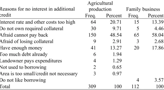
We also asked the households that reported they did not want more credit why they were not interested in more credit, allowing the households to give up to three responses. The analysis of these responses (table 5) indicates that the level of credit rationing might actually be higher. Only 18% of the responses for agricultural production could be associated with a real absence of credit need (have enough money, landowner pays expenditures, too much debt already, not used to borrowing, credit not necessary). Thirty households reported that they did not own the required collateral and 64 reported that the interest and other costs were too high, indicating some extent of price rationing.
If we consider that the households that report that interest rates and other costs were too high or that they didn’t own the required collateral are credit constrained, we
28 This has lead to 14 reclassifications of households as agriculture production credit constrained, 1 as
non-agricultural business credit constrained and 19 as consumption credit constrained. Among households that were not agricultural producers, 4 expressed agriculture related credit need and 2 households that were not operating any family business reported business related credit need.
29 This figure doesn’t derive directly from table 4 as some households that are engaged in both agricultural
and non agricultural activities can be constrained on one of their production activity only but be counted as constrained in their production decisions.
observe a sharp increase in the level of credit rationing:30 59% of the agricultural producers31 and 43% of the non agricultural producer would be constrained.
Table 5 Reasons why the households didn’t want more credit to finance their production
Agricultural
production Family business
Reasons for no interest in additional
credit Freq. Percent Freq. Percent
Interest rate and other costs too high 64 20.71 15 13.39
Do not own required collateral 30 9.71 5 4.46
Afraid cannot pay back 150 48.54 65 58.04
Afraid of losing collateral 9 2.91 3 2.68
Have enough money 41 13.27 20 17.86
Too much debt already 6 1.94
Landowner pays expenditures 4 1.29
Not used to borrowing 2 0.65
Area is too small/credit not necessary 3 0.97
Do not like borrowing 4 3.57
Total 309 100 112 100
This reclassification of production-constrained status would lead to an increase in the overall level of credit rationing from 39% up to 52%. If the credit market is competitive, interest rates should reflect the risk faced by the lender and only changes in the level of risk of the demand side can reduce price rationing. The high proportion of households that report that they would not have used more credit because interest rates were too high suggest a need for interventions such as implementation of risk reducing agricultural technologies or credit bureaus aimed at reducing risk. In the remainder of the paper, we will use the direct answers of the households regarding their marginal credit needs and use the variables as defined in table 4.
Households can have unsatisfied credit needs other than production or non-food consumption credit needs as revealed by the response to the question on the use of the
30 Households that reported that they did not want more credit for consumption were not asked why they
were not interested in more credit for consumption.
31 Two households reported that the interest rates and other costs were too high but also that either it had
enough money or that it already had too much deb. These two households were not reclassified as credit constrained.
credit that the household needed in the past year but didn’t ask for (see above).32 Around 20% of the households (104 households) reported that they needed credit that they didn’t ask for food consumption.
Table 6 Purpose of the ‘discouraged’ loan needs
Purpose of the discouraged loans Freq. Percent
Food expenditures Food consumption 104 28.73
Education 29 8.01 Health 25 6.91 Clothing 1 0.28 Traveling expenses 4 1.1 Marriage/family events 4 1.1 Non-food expenditures
Improving dwelling unit 16 4.42
Means of transport 4 1.1
Assets and consumer
durables Consumer durables 29 8.01
Farm inputs 66 18.23
Farm equipments 2 0.55
Purchase animals 18 4.97
Agricultural production
Purchase/lease of agricultural lands 6 1.66
Purchase of goods for trade 24 6.63
Purchase of inputs and working capital 19 5.25
Purchase of equipment 3 0.83
Non-agricultural business
Additional capital for business 1 0.28
Refinancing Debt repayment/refinancing 7 1.94
Total 362 100
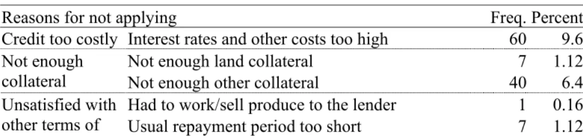
The analysis of the reasons why the households did not apply for these loans indicate that most of these are discouraged credit transactions:
Table 7 Reason why the households didn’t apply for some loan need
Reasons for not applying Freq. Percent
Credit too costly Interest rates and other costs too high 60 9.6
Not enough land collateral 7 1.12
Not enough
collateral Not enough other collateral 40 6.4
Had to work/sell produce to the lender 1 0.16
Unsatisfied with
other terms of Usual repayment period too short 7 1.12
32 303 (53%) of the households reported that they needed credit in the past year that they didn’t ask for and
Usual frequency of installment inadequate 2 0.32
Too much time before the credit is given 4 0.64
Did not like to mortgage 3 0.48
Too many requirements 6 0.96
Didn't like the terms & conditions of the loan 2 0.32
Loan need too small 6 0.96
the contract
Loan need too large 1 0.16
Lender too far 7 1.12
No available
lender Did not know anybody who could lend me 8 1.28
Afraid to lose collateral 16 2.56
Afraid to incur extra fees for late repayment 179 28.64
Afraid of the consequences of
credit Afraid of having bad repayment reputation 50 8
Think lender would not approve loan 18 2.88
Not able to meet with lender/ ashamed to borrow 2 0.32
Self-selection, other
Did not understand the agreement 1 0.16
Too much debt already 63 10.08
No stable job/income to pay loan 10 1.6
Found work/receive remittance from children 9 1.44
Spouse did not give consent 1 0.16
Disliked borrowing 67 10.72
No interest in additional loan
No longer need any loan 55 8.8
Total 625 100
We also asked the households whether any loan they applied for in the past year had been rejected. Thirty one percent of the households (180) were rejected for at least one loan and only 38% of these were able to get one of these rejected loans from another lender. In an attempt to provide a global picture of credit constraints we considered the following types of households as credit constrained:33 (1) households that experienced at least one rejection for a loan they had asked for, and were not able to get any of these loans elsewhere; and (2) households that reported they needed credit for which they did not apply. 34 Adding to these constrained households (52%) the households that reported they would have liked more credit for agricultural production, for their family business or for
33 In the regressions however, we use the variables of credit constraints differenciated by use as defined in
table 4.
34 Fifty households expressed a latent credit need for which they did not apply, but would not have been
interested in obtaining a loan if credit had been available to them. These households were not considered as credit constrained. Their answer to the question on why they did not apply was one of the following: they disliked borrowing, they had too much debt already, they found work or received remittances from their children, the spouse did not consent, or they no longer needed any loan.
their non-food expenditures, we reach a total number of 372 credit-constrained households, corresponding to 65% of our sample.
We will concentrate our subsequent analysis on credit constraints for production or for non-food expenditures.
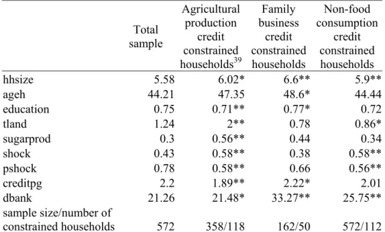
4.3. Selected descriptive statistics of the survey households
Table 8 presents the definitions, means, standard deviations, minimum and maximum of the variables used for our estimations of credit constraints and table 9 presents the means of these variables for the total sample, for agricultural producers, for family business owners and for households engaged in both farm and non farm production. Households engaged in agricultural or non-agricultural production tend to be larger and have an older household head. Smaller households typically young
households35 who typically start working for somebody else before being able to
accumulate assets and start a business on their own. Although the Philippine constitution provides for universal primary education, only 50% of the households in which all members aged 14 and above have at least six years of schooling. In 29% of the households, only half or less of the members above 14 years old have at least six years of education. 27% of the household heads had 4 years of education or less in our sample. There is substantial variation in the area of titled land owned by the farming households with 25% of the farming households owning more than 75% of the total titled land area of farming households. The Gini coefficient of 0.96 indicates that landownership concentration is very high. There are on average more households operating family business in barangays where governmental or NGO credit programs operate. These credit programs usually support livelihood activities and seem to have been successful in
expanding off-farm businesses.36 Agricultural producers are on average closer to a
commercial or rural bank than non-farm households.
35 A test of difference of means for the age of the household head reveals that non-producers households
have significantly younger heads.
Table 8 Description and descriptive statistics, the whole sample
Variables Description Mean Std.Dev. Min Max
hhsize Size of the household 5.58 2.236 1 20
ageh Age of the household head in years 44.21 13.629 17 78
education
Proportion of household members over 14 years old with at least six years of
education
0.75 0.311 0 1 tland Area of titled land owned by the household, in hectares 1.24 3.428 0 42.65 sugarprod Dummy=1 if the area planted to sugar by the household is at least 0.25 hectares 0.3 0.457 0 1 shock Number of negative shocks experienced by the household between 2001 and 2003 0.43 0.698 0 4 pshock
Number of shocks that have made 10% or more of the barangay households worse off during the years 2001 to 2003
0.78 1.005 0 3 creditpg
Number of NGO or governmental programs that provide credit services in the barangay
2.2 1.801 0 8 dbank Distance to the nearest commercial or rural bank, in kilometers 21.26 32.228 0 100
Table 9 Comparison of means based on productive activity
Total sample Agricultural producer households Households operating a family business Households engaged in farming and family business hhsize 5.58 5.78** 5.91** 6.1** ageh 44.21 46.74*** 46.57** 47.76** education 0.75 0.75 0.83*** 0.75** tland 1.24 1.98*** 1.23 1.87** sugarprod 0.3 0.4737 0.37** 0.57*** shock 0.43 0.44 0.38 0.4 pshock 0.78 0.77 0.81 0.77 creditpg 2.2 2.22 2.55** 2.65** dbank 21.26 18.05** 23.74 23.53
***Difference of means significant38 at the 1% level; **significant at the 5% level; * significant at the 10% level.
37 Test of difference of means not performed since non-agricultural households cannot be sugar producers. 38 Difference in the means of farm households compared to non-farm households for example.