Aggregation of Statistical Data from Passive Probes: Techniques and Best Practices

HAL Id: hal-01396470

https://hal.archives-ouvertes.fr/hal-01396470

Submitted on 14 Nov 2016

HAL is a multi-disciplinary open access

archive for the deposit and dissemination of

sci-entific research documents, whether they are

pub-lished or not. The documents may come from

teaching and research institutions in France or

abroad, or from public or private research centers.

L’archive ouverte pluridisciplinaire HAL, est

destinée au dépôt et à la diffusion de documents

scientifiques de niveau recherche, publiés ou non,

émanant des établissements d’enseignement et de

recherche français ou étrangers, des laboratoires

publics ou privés.

Distributed under a Creative Commons Attribution| 4.0 International License

Aggregation of Statistical Data from Passive Probes:

Techniques and Best Practices

Silvia Colabrese, Dario Rossi, Marco Mellia

To cite this version:

Silvia Colabrese, Dario Rossi, Marco Mellia. Aggregation of Statistical Data from Passive Probes:

Techniques and Best Practices.

6th International Workshop on Traffic Monitoring and

Analy-sis (TMA), Apr 2014, London, United Kingdom. pp.38-50, �10.1007/978-3-642-54999-1_4�.

�hal-01396470�

Aggregation of statistical data from passive probes:

Techniques and best practices

Silvia Colabrese1_{, Dario Rossi}1_{, Marco Mellia}2

1

Telecom ParisTech, Paris, France - {silvia.colabrese,dario.rossi}@enst.fr

2

Politecnico di Torino, Torino, Italy - marco.mellia@polito.it

Abstract. Passive probes continuously generate statistics on large number of metrics, that are possibly represented as probability mass functions (pmf). The need for consolidation of several pmfs arises in two contexts, namely: (i) when-ever a central point collects and aggregates measurement of multiple disjoint van-tage points, and (ii) whenever a local measurement processed at a single vanvan-tage point needs to be distributed over multiple cores of the same physical probe, in order to cope with growing link capacity.

In this work, we take an experimental approach and study both cases using, when-ever possible, open source software and datasets. Considering different consoli-dation strategies, we assess their accuracy in estimating pmf deciles (from the 10th to the 90th) of diverse metrics, obtaining general design and tuning guide-lines. In our dataset, we find that Monotonic Spline Interpolation over a larger set of percentiles (e.g., adding 5th, 10th, 15th, and so on) allow fairly accurate pmf consolidation in both the multiple vantage points (median error is about 1%, maximum 30%) and local processes (median 0.1%, maximum 1%) cases.

1

Introduction

Passive probes collect a significant amount of traffic volume, and perform statistical analysis in a completely automated fashion. Very common statistical outputs include, from the coarsest to the finest grain: raw counts, averages, standard deviations, higher moments, percentiles and probability mass functions (pmf). Usually, computations are done locally at a probe, though there may be cases where the need for consolidation of multiple statistics, in a scalable and efficient way, arise.

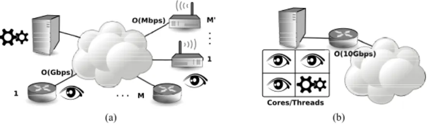
We would now like to mention two completely orthogonal scenarios where this need arises, which we describe with the help of Fig. 1. In the figure, a number of monitors (denoted with an eye) generate statistics that are fed to a collector (denoted with gears) for consolidation. The figure further annotates the amount of traffic to be analyzed that flows across each monitored link.

First, in case of multiple vantage points of Fig. 1-(a), consolidation of several data sources is desirable as it yields a more statistically representative population sample. In cases where these probes are placed at PoP up in the network hierarchy, a limited number of M monitors suffices in gathering statistics representative of a large user pop-ulation. However, in cases where probes represent individual house-holds, the number of M0 monitors possibly grows much larger. As monitors and collector are physically disjoint, statistics have to be transferred to the collector – a potential system bottleneck.

1 M' 1 . . . _M . . . O(Gbps) O(Mbps) O(10Gbps) Cores/Threads (a) (b)

Fig. 1.Consolidation scenarios: statistical data is either produced by (a) multiple physically dis-joint probes (heterogeneous traffic), or (b) a single multi-threaded probe (homogeneous traffic).

Second, even in the case of a single vantage point of Fig. 1-(b), due to the sheer amount of traffic volume, it may be necessary to split traffic processing over multi-ple independent cores. Considering a high-end off-the-shelf multi-core architecture, the number of available CPUs limits the number of parallel processes to a few handful (we are not considering, at this stage, GPU-based architectures). In contrast to the previous case, monitors and collector are in this case colocated – so that processing power, rather than transfer of statistical data, becomes a potential system bottleneck.

While these two scenarios seem rather different at first sight, we argue that they translate into similar constraints. Thus we suggest using a single, flexible methodology to cope with both cases. In the case of multiple vantage points, using the least possible amount of statistical data is desirable to avoid a transfer bottleneck. In the case of par-allel processing at a single vantage point, elaborating the least possible amount of data is desirable to limit the computational overhead tied to the consolidation process.

The above constraints possibly trade-off with the amount of data that is required to meet the desired accuracy level in the consolidation process, which additionally de-pends on the specific statistic of interest. Whenever the statistic X to be consolidated has the coarsest (i.e., count, averages or second moment) or finest (full pmf) grain, then the full set{Xj}Mi=j of statistics gathered over all M vantage points is needed for the

consolidation process: the consolidation process then trivially combines these affine in-puts (e.g., averaging the average, or maximum over all maximums, or summing the pmf frequency counters), weighting them on the ground of the amount of traffic Tithat each

vantage point represents wi = Ti/

∑M j=1Tj.

Instead, consolidation of intermediate-grain statistics, such as higher moments or quantiles of the distribution, raises a more interesting and challenging problem. For example, consider the problem of accurate estimation of the 90th percentile of a given metric, and assume for the sake of simplicity that all vantage points correspond to the same amount of traffic (i.e., unit weights wi = 1∀i). It is clear that, while the fine

grained knowledge of the pmf at all vantage points is not necessary to estimate the 90th percentiles of the aggregate pmf, the mere knowledge of the 90th percentiles over all vantage points is not sufficient.

While our aim is to propose a general methodology, and to obtain general design and tuning guidelines, in this paper we report on a specific instance of metrics gathered through the Tstat [1] measurement tool, a passive flow-level monitor that we developed

over the last years [8]. We point out that, as other tools, Tstat produces both detailed flow-level logs at several layers (e.g, transport, application) as well as periodic statis-tics, stored as a Round Robin Database (RRD). While statistics are automatically com-puted, they offer only limited flexibility providing a breakdown depending on the traffic direction (e.g., client-2-server vs server-2-client, incoming vs outgoing). Hence, while aggregate statistics are useful, as they offer a long-lasting automatic of several networks indicator, in order to study correlation or conditioned probabilities across metrics, logs are ultimately needed. As such, consolidation of automatic statistics possibly tolerate slight inaccuracies if that provides sizable savings in terms of computational power or bandwidth.

In this paper, we focus on the estimation of pmf deciles (from the 10th to the 90th), considering vantage points located into rather different networks (open dataset when-ever possible) and a large span of metrics (at IP, TCP and UDP layer). We employ different consolidation strategies (e.g., Linear vs Spline interpolation techniques) and a varying amount of information (i.e., considering the deciles, or also additional quantiles of the distribution). In the remainder of this paper, we outline the methodology (Sec. 2) and dataset (Sec. 3) we follow in our experimental campaign (Sec. 4). A discussion of related work (Sec. 5) and guidelines (Sec. 6) concludes the paper.

2

Methodology

2.1 Features

The most concise way to represent a pmf or the related distribution is by the use of percentiles. Tstat computes two kinds of percentiles:

Per-flow percentiles.For these fine-grained metrics, Tstat employs an online tech-nique based on constant-space data structures (namely, PSquare [13]): percentiles of per-flow metrics are then stored in flow-level logs. Though PSquare is very ef-ficient in both computational complexity and memory footprint (namely, requiring only 5 counters per percentile), due to the large number of flows it is only seldom used (e.g., to measure 90th, 95th and 99th percent of queuing delay to measure bufferbloat [5]).

Aggregated percentiles.For this coarse grain metric, Tstat employs standard fixed-width histograms: percentiles of the distribution are then evaluated with linear in-terpolation, and stored in Round Robin Databases (RRD). Generally, each flow contributes one sample to the aggregate distribution, and several breakdowns of the whole aggregated are automatically generated depending on the traffic direction (e.g., client-2-server vs server-2-client, incoming vs outgoing).

For reasons of space, we are unable to report the full list of traffic features tracked by Tstat as aggregate metrics (for a detailed description, we refer the reader to [1]). We point out that these span multiple layers, from network (i.e., IP) to transport (i.e., TCP, UDP, RTP) and application layers (e.g., Skype, HTTP, YouTube). Since not all kinds of traffic are available across all traces (e.g., no Skype or multimedia traffic is present in the oldest trace in our dataset), we only consider the IP, TCP and UDP metrics.

Fig. 2.Synopsis of the experimental workflow

2.2 Consolidation workflow

In this work, we focus on the coarse-grain dataset and estimate quantiles of the distri-bution. We describe our workflow with the help of Fig. 2, considering a generic traffic feature. Shaded gray blocks are the input to our system. Such blocks represent quantiles vectors qi, gathered from multiple (local or remote) Tstat probes running at location i,

with i ∈ [1, NP]. We interpolate each quantile vector to get a cumulative distribution

function (CDF). These functions are weighted by the amount of traffic they represent (weights can be computed in terms of flows, packets or bytes), and added to get the total CDF. Finally, as output of our workflow, we obtain the consolidated qi deciles vector

from the total CDF with the bisection method.

It is worth noticing that the procedure implicitly yields continuous CDF functions, whereas the empirical CDFs computed through Tstat histograms are piecewise constant functions instead. To cope with this, it would be possible to quantize a posteriori the gathered quantiles for discrete variables (e.g., packet length, IP TTL). However, we neglect this step because (i) we aim for a fully automated process, whereas this per-feature optimization would require manual intervention and (ii) we expect the impact due to missed rounding of integer values to be minor anyway.

Finally, the consolidated continuous output is compared to the real quantiles q_iof the aggregated distribution, obtained from running Tstat on the aggregated traces. In what follows, we evaluate the accuracy of the overall workflow via the relative error

erri= (qi− ˜qi)/˜qiof the consolidation process.

2.3 Interpolation

To obtain the CDFs, we employ two kinds of interpolation.

Linear (L).For each couple of consecutive deciles, linear interpolation reconstructs the CDF by using an affine equation y = mx + q. Being (qi, pi) and (qi+1, pi+1)

the given points, m = pi+1−pi

qi+1−qi and q = pi. If the function to approximate were

continuous in both their first and second derivative (i.e., f ∈ C2_{) then we could} upper bound the error through the Rolle’s Theorem. Yet, these assumptions do not

hold in the majority of real cases, so that we can just expect that, the steeper the first derivative, the higher the errors.

Monotonic Spline (S).Cubic Splines are Piecewise polynomial functions with n = 3. Given that CDF (a)≤ CDF (b) when a ≤ b we need to ensure the monotonicity of the data. This constraint is met employing the Piecewise Cubic Hermite Interpo-lating Polynomial [9]. The obtained polynomial is∈ C1: i.e., the first derivative is continuous, whereas continuity of the second derivative is not guaranteed.

2.4 Input vs Output

As output, we are interested in evaluating all deciles of the distribution: along with min-imum and maxmin-imum values, these represent compact summaries of the whole CDF. Our methodology exploits quantiles to reconstruct the distributions, and operate over CDFs. In principle, this allows to gather any set of output quantiles from CDFs reconstructed from a set of different input quantiles. In this work, we consider two cases:

Single (S).In the simplest case, we consider deciles as both input and output of our workflow.

Double (D).We argue that CDF interpolation can benefit from a larger number of samples (i.e., knots in Spline terms), providing a more accurate description for the intermediate consolidation process. As such, we additionally consider the possi-bility of using additional intermediate (i.e., 5th, 15th, 25th to 95th) quantiles of the distribution (i.e., that carry a double amount of information with respect to the previous case).

While the above two scenarios are not fully representative of the whole input vs output space (where in principle the full cross-product of input vs output quantiles sets could be considered) however, we point out that they already provide insights about the value of additional input information. We expect these settings to quantify the relative importance of information available at the ingress of the system, with respect to the specific methodology used for, e.g., interpolation in the workflow.

3

Datasets

We use several traces, some of which are publicly available. Vantage points pertain to different network environments (e.g., Campus and ISP networks), countries (e.g., EU and Australia) and have been collected over a period of over 8 years. This extreme heterogeneity attempts to obtain conservative accuracy values: our expectation is that, as not only the environment and the geography largely differ, but also since the traffic patterns, application mixtures and Internet infrastructure have evolved, this setup should be significantly more challenging than a typical use case. In more details, traces refer to:

Campus.Captured during 2009 at University of Brescia (UniBS), this publicly avail-able trace [3] is representative of a typical data connection to the Internet. LAN users can be administrative, faculty members and students.

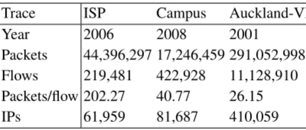
Table 1.Summary of dataset used in this work.

Trace ISP Campus Auckland-VI

Year 2006 2008 2001

Packets 44,396,297 17,246,459 291,052,998 Flows 219,481 422,928 11,128,910 Packets/flow 202.27 40.77 26.15

IPs 61,959 81,687 410,059

ISP.Collected during 2006 from one of the major European ISP, which we cannot cite due to NDA, offering triple-play services (Voice, Video/TV, Data) over broadband access. ISP is representative of a very heterogeneous scenario, in which no traffic restriction are applied to customers.

Auckland. Captured during 2001 at the Internet egress router of the University of Auckland, this publicly available trace [2] enlarges the traffic mix and temporal span of our dataset.

While we are unable to report details of the above dataset for lack of space, we point out that these are available at the respective sites [2, 3], of which we additionally provide statistics on [16]. To simplify our analysis, we consider a subset of about 200,000 ran-domly sampled flows for each trace1, which implies equal weights. Given that each flow represents a sample for the CDF, we observe that CDFs are computed over a statistically significant population.

4

Experiments

4.1 Scenario and settings

Starting from the above dataset, we construct two consolidation scenarios: for the local parallel processing case (Homogeneous), we uniformly sample flows from the ISP trace, that we split into N ∈ [2, 8] subtraces (in the N = 8 case, the population accounts to about 25,000 flows for each individual CDF). For the multiple remote vantage points case (Heterogeneous), we instead consider the three traces (about 600,000 flows).

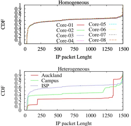
To give a simple example of the variability of metrics we report in Fig. 3 the distri-bution of an IP-level (i.e., IP packet length) metric in the parallel processing (left) and multiple vantage point (right) scenarios. As expected, differences in the parallel pro-cessing case are minor: as sampling is uniform, each of the N subsamples already yields a good estimate of the overall aggregate distribution. Conversely, significant differences appear in the multiple vantage points scenario: in this case, the application mixture im-pacting the relative frequency of packet sizes (e.g., 0-payload ACK vs small-size VoIP packets vs full-size frames data packets). has significantly evolved2.

1

Actually, we consider the full ISP trace, so sample size is 219,481 flows for each trace

2

Additionally, changes in the MTU size due to Operating System and Internet infrastructure evolution are possible causes, that would however need further verification.

0

0.1

0.2

0.3

0.4

0.5

0.6

0.7

0.8

0.9

1

0

250

500

750

1000 1250 1500

CDF

IP packet Lenght

Homogeneous

Core-05

Core-06

Core-07

Core-08

0

0.1

0.2

0.3

0.4

0.5

0.6

0.7

0.8

0.9

1

0

250

500

750

1000 1250 1500

CDF

IP packet Lenght

Homogeneous

Core-01

Core-02

Core-03

Core-04

0

0.1

0.2

0.3

0.4

0.5

0.6

0.7

0.8

0.9

1

0

250

500

750

1000 1250 1500

CDF

IP packet Lenght

Heterogeneous

Auckland

Campus

ISP

Fig. 3.Example of variation of an IP-level metric (i.e., IP packet length) in Homogeneous vs Heterogeneous settings.

Overall, we consider four consolidation settings, arising from different combina-tion of interpolacombina-tion techniques and inputs, namely: Linear Simple (LS), Linear Double (LD), Spline Simple (SS), Spline Double (SD) – that correspond to different computa-tional complexity and data amount settings. Our aim is to assess the extent of accuracy gains that can be gathered through the use of more complex interpolation techniques, or through the exchange of a larger amount of information.

4.2 Methodology tuning

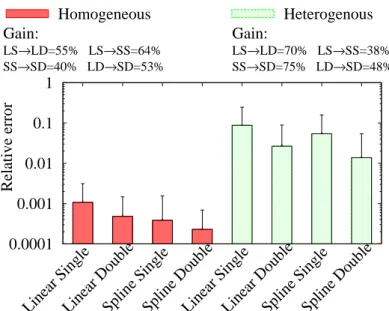
We first assess the consolidation accuracy in the LS, LD, SS, SD settings, for both homogeneous and heterogeneous scenarios. We report the average error (with standard deviation bars) in Fig. 4. The plot is additionally annotated with the accuracy gain over the naive LS setting.

First, notice that in the homogeneous scenario the error is very low, but grows of about two orders of magnitude in our heterogeneous one (where all techniques are largely ineffective). Second, it can be seen that while Spline interpolation has an

0.0001

0.001

0.01

0.1

1

Linear Single

Linear Double

Spline Single

Spline Double

Linear Single

Linear Double

Spline Single

Spline Double

Relative error

Gain:

Homogeneous

Heterogenous

Gain:

Fig. 4.Methodology tuning: Consolidation error in the Linear vs Spline, Single vs Double case for the IP TTL metric considering Homogeneous and Heterogeneous cases

portant impact (at least 38%), doubling the amount of quantiles however has an ever higher impact. Moreover, this is especially true in the more difficult heterogeneous sce-nario, where gains are in excess of 70% when interpolation happens over a denser set of quantiles, whereas Spline interpolation gain at most 48%. While this is an interest-ing observation, it raises an important question, which we leave for future research: namely, to precisely assess in which conditions, over all metrics and input-output possi-bilities, having a larger amount of information is more beneficial than employing more sophisticated interpolation techniques.

As a consequence, in what follows we limitedly consider the SD setting (i.e., Spline interpolation over Double set of quantiles), as it yields to the best consolidation results.

4.3 Breakdown

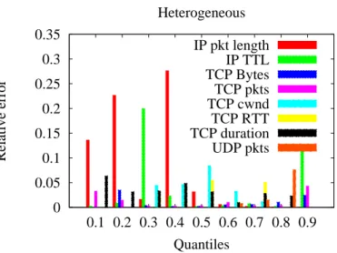
Next, we show a per-percentile per-metric breakdown of the relative error in Fig. 5. For the sake of illustration, we consider a few metrics that are representative of different layers (IP, TCP, UDP). To get conservative results, we consider only the most challeng-ing heterogeneous scenario. As it can be expected, errors are not tied to a particular decile, as the error is rather tied to the steepness of the change in the CDF around that decile for that particular metric. For exanoke, considering the IP packet length metric, due to significant CDF differences across traces depicted early in Fig. 3-(b), it can be expected that deciles below the median are hard to consolidate: this is reflected by large errors for the corresponding deciles in Fig. 5.

0

0.05

0.1

0.15

0.2

0.25

0.3

0.35

0.1 0.2 0.3 0.4 0.5 0.6 0.7 0.8 0.9

Relative error

Quantiles

Heterogeneous

IP pkt length

IP TTL

TCP Bytes

TCP pkts

TCP cwnd

TCP RTT

TCP duration

UDP pkts

Fig. 5.Methodology tuning: Breakdown of relative error under the Spline Double consolidation strategy for different percentiles and metrics under the Heterogeneous case.

As we previously have observed, rather than trying harder to correct these esti-mation errors a posteriori (i.e., using Spline instead of Linear interpolation), greater accuracy is expected to come only at a price of a larger amount of information (i.e., quantiles for CDF interpolation), and are ultimately tied to the size of the binning strat-egy in Tstat. Otherwise stated, our recommendation is to selectively bias the amount of quantiles: instead of indiscriminately increasing the amount of quantiles for all metrics, one could use denser quantiles (or finer binning) only for metrics with a high subjective value in the scenario under investigation. This could be facilitated by a integer “overfit” factor extending beyond the values Simple(=1), Double (=2) explored in this work, that could be easily set during an initial probe configuration phase.

4.4 Homogeneous vs Heterogeneous

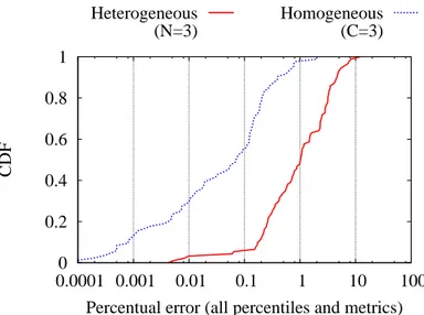
We now report a complete CDF of the relative error over all Tstat metrics and per-centiles in Fig. 6, where we compare the heterogeneous and homogeneous case (to get a fair comparison, we consider only N = 3 subsets in both cases). As previously ob-served, there is a sizable difference in terms of accuracy, with median relative error in the homogeneous (heterogeneous) cases of 0.1% (1%), and maximum error of 1% (30%). Notice that we are considering Spline with Double quantiles, otherwise errors in the heterogeneous settings could grow even further. It follows that, while the con-solidation appears to be rather robust in homogeneous settings, it may serve as a mere visual indication depending on the specific metric and decile (recall Fig. 5), but cannot otherwise be considered reliable (or, at least, a calibration phase is needed in to assess the relative error with any different set of remote vantage points).

0

0.2

0.4

0.6

0.8

1

0.0001 0.001 0.01

0.1

1

10

100

CDF

Percentual error (all percentiles and metrics)

Heterogeneous

(N=3)

Homogeneous

(C=3)

Fig. 6.Accuracy of Double Spline consolidation strategy: CDF of relative error, all metrics and deciles, in the homogeneous vs heterogeneous scenarios.

4.5 Parallel local probes

Finally, we verify the effect of splitting the trace in an arbitrary number of parallel pro-cesses: we do so by artificially splitting the ISP trace into multiple N ∈ [2, 8] subtraces, and process them independently. In principle, it would be desirable to use an arbitrarily high number of cores, as this would allow the monitoring tool scale with the link load. At the same time, we expect consolidation accuracy to decrease with growing N, so that an empirical assessment of its error is mandatory, so to gauge to what extent paral-lelization could compromise the accuracy of the statistical results. Results are reported in Fig. 7 averaged over all metrics (bars report this time the error variance, as the stan-dard deviation of a numbere∈ [0, 1] produce otherwise a too large visual noise). It can be seen that the error, though very limited for any N > 1, grows logarithmically with

N . This implies that the largest accuracy loss happens whenever a monolithic process

is split into 2 parallel processes, suggesting that a monitoring tool can safely scale to N cores.

5

Related work

Statistical data processing and aggregation in distributed systems is surely not a novel research field. Yet, in the telecommunication network domain, the problem has so far been treated in rather different settings (e.g., sensor vs peer-to-peer networks).

From a system level, this is easily understood since only very recent work offered high-speed packet capture libraries [4, 10, 17] enabling parallel processing of network traffic. Work such as [10] or [6] leverage this possibility for packet forwarding or traffic

0.12

0.13

0.14

0.15

0.16

0.17

1

2

3

4

5

6

7

8

Relative error [%]

Number of cores

Homogeneous

Fig. 7.Accuracy of Double Spline consolidation strategy: Average relative error for varying num-ber of cores N in the homogeneous scenario.

classification respectively, though work that focuses on traffic monitoring is closer to ours [7, 12, 15]. For example, [7] focus on making log storage cope with line rate, deferring the process of analysis and consolidation as a offline process. Other recent work defines fully-fledged frameworks for distributed processing [12, 15]. While these systems have merits, they are far more general than the issue studied in this work. Yet performance analysis is limited to show-case functionality of the tools, though neither practical algorithms nor guidelines are given for our problem at hand.

In the distributed system settings, generally the focus has been on either (i) com-pact and efficient algorithms and dat structures for quantile estimation, or on (ii) proto-cols to compute an estimate of the entire distribution in a decentralized and efficient manner. As for (i), among the various techniques, a particular mention goes to the PSquare method [13], that is still considered as the state of the art [14,18], and is imple-mented in Tstat. As for (ii), [11] proposes a gossip protocol to distribute computation of Equi-Width and Equi-Depth histograms, evaluating the convergence speed (measured in number of rounds) and quality (Kolmogorov-Smirov distance between the actual and estimated distributions). In our case, a single collector point allow us to minimize the communication overhead and perform consolidation in a single round. More recently, a number of approaches are compared in [19], that would be interesting to adapt and specialize to our settings.

Finally, it is worth mentioning that this problem is orthogonal to the widely used technique of traffic sampling, with which techniques considered in this work are further-more inter-operable. Indeed, traffic sampling (e.g., at flow level) is useful in reducing the sheer volume of traffic flows that have to be processed at a single probe; yet, flow sampling does not affect the volume of statistical data that is produced by the monitors,

and that is ultimately fed to collectors. Recalling our use cases, flow sampling may re-lieve CPU bottlenecks of the multi-process case of Fig. 1-(b), but it does otherwise not affect the amount of statistical data reaching the collector in Fig. 1-(a). To this latter end, a spatial sampling among monitors could reduce the amount of statistical data fed to the collector, though this could tradeoff with the representativeness of the data – an interesting question that deserves further attention.

6

Conclusions

In this work we address the problem of consolidating statistical properties of network monitoring tools coming from multiple probes, either as a result of parallel processing at a single vantage point, or collected from multiple vantage points. Summarizing our contributions, we find that:

– as it can be expected, while consolidation error is practically negligible in the case of local processes, where statistics are more similar across cores (median error is about 0.1% and maximum 1%), it is however possibly rather large in the case of multiple disjoint vantage points with diverse traffic natures (median error is about 1% and maximum 30%, though it possibly exceeds 100% for naive strategies); – the use of intermediate pmf quantiles (e.g., 5th, 15th, and so on), is desirable as it

significantly improves accuracy (up to 75% in the case of multiple vantage points), even though it tradeoffs with communication and computational complexity; – interpolation via Splines is preferable over simpler Linear interpolation, as it yields

to an accuracy gain of over 40%;

– the error in case of parallel processing grows logarithmically with the number of processes, suggesting parallel processing tools to be a viable way to cope with growing link capacity at the price of a tolerable accuracy loss.

As part of our ongoing work, we are building this consolidation system as a general tool, able to work on RRD databases. We also plan to extend our analysis of the accuracy to cover a larger set of input vs output features combination, and to more systematically analyze benefits of interpolation vs additional information in these broader settings.

Acknowledgement

This work has been carried out at LINCS http://www.lincs.fr and funded by EU under FP7 Grant Agreement no. 318627 (Integrated project “mPlane”).

References

1. http://tstat.tlc.polito.it.

2. Auckland traces. http://www.wand.net.nz/.

3. Unibs traces. http://www.ing.unibs.it/ntw/tools/traces/.

4. N. Bonelli, A. D. Pietro, S. Giordano, and G. Procissi. Pfq: a novel engine for multi-gigabit packet capturing with multi-core commodity hardware. In Passive and Active Measurement

5. C. Chirichella and D. Rossi. To the moon and back: are internet bufferbloat delays really that large. In IEEE INFOCOM Workshop on Traffic Measurement and Analysis (TMA), 2013. 6. P. S. del Rio, D. Rossi, F. Gringoli, L. S. L. Nava, and J. Aracil. Wire-speed statistical

classifi-cation of network traffic on commodity hardware. In ACM SIGCOMM Internet Measurement

Conference (IMC), 2012.

7. L. Deri, A. Cardigliano, and F. Fusco. 10 gbit line rate packet-to-disk using n2disk. In IEEE

INFOCOM workshop on Traffic Monitoring and Analysis (TMA), 2013.

8. A. Finamore, M. Mellia, M. Meo, M. Munafo, and D. Rossi. Experiences of internet traffic monitoring with tstat. IEEE Network, 2011.

9. F. N. Fritsch and R. E. Carlson. Monotone piecewise cubic interpolation. SIAM Journal on

Numerical Analysis, 17(2):238–246, 1980.

10. S. Han, K. Jang, K. Park, and S. Moon. Packetshader: a gpu-accelerated software router. In

ACM SIGCOMM, 2010.

11. M. Haridasan and R. van Renesse. Gossip-based distribution estimation in peer-to-peer net-works. In USENIX Internet Peer-to-Peer Symposium (IPTPS), 2008.

12. F. Huici, A. Di Pietro, B. Trammell, J. M. Gomez Hidalgo, D. Martinez Ruiz, and N. d’Heureuse. Blockmon: A high-performance composable network traffic measurement system. ACM SIGCOMM Computer Communication Review, 42(4):79–80, 2012.

13. R. Jain and I. Chlamtac. The p2 _{algorithm for dynamic calculation of quantiles and}

his-tograms without storing observations. Communications of the ACM, 28(10):1076–1085, 1985.

14. J. Kilpi and S. Varjonen. Minimizing information loss in sequential estimation of several quantiles. Technical Report, 2009.

15. C. Lyra, C. S. Hara, and E. P. Duarte. Backstreamdb: A distributed system for backbone traffic monitoring providing arbitrary measurements in real-time. In Passive and Active

Mea-surement (PAM), 2012.

16. A. Pescape, D. Rossi, D. Tammaro, and S. Valenti. On the impact of sampling on traffic monitoring and analysis. International Teletraffic Congress (ITC22), 2010.

17. L. Rizzo. Revisiting network i/o apis: the netmap framework. Commun. ACM, 55(3):45–51, Mar. 2012.

18. H. Wang, F. Ciucu, and J. Schmitt. A leftover service curve approach to analyze demulti-plexing in queueing networks. In VALUETOOLS, 2012.

19. L. Wang, G. Luo, K. Yi, and G. Cormode. Quantiles over data streams: an experimental study. In ACM SIGMOD, 2013., 2013.