O
pen
A
rchive
T
OULOUSE
A
rchive
O
uverte (
OATAO
)
OATAO is an open access repository that collects the work of Toulouse researchers and
makes it freely available over the web where possible.
This is an author-deposited version published in :
http://oatao.univ-toulouse.fr/
Eprints ID : 6278
To link to this article : DOI:10.1109/TIP.2012.2199505
URL : http://dx.doi.org/10.1109/TIP.2012.2199505
To cite this version : Park, Se Un and Dobigeon, Nicolas and Hero,
Alfred O. Semi-blind sparse image reconstruction with application
to MRFM. (2012) IEEE Transactions on Image Processing, vol. 21
(n° 9). pp. 3838-3849. ISSN 1057-7149
Any correspondence concerning this service should be sent to the repository
administrator:
[email protected]
㩷Semi-Blind Sparse Image Reconstruction
With Application to MRFM
Se Un Park, Nicolas Dobigeon, Member, IEEE, and Alfred O. Hero, Fellow, IEEE
Abstract— We propose a solution to the image deconvolution problem where the convolution kernel or point spread function (PSF) is assumed to be only partially known. Small pertur-bations generated from the model are exploited to produce a few principal components explaining the PSF uncertainty in a high-dimensional space. Unlike recent developments on blind deconvolution of natural images, we assume the image is sparse in the pixel basis, a natural sparsity arising in magnetic resonance force microscopy (MRFM). Our approach adopts a Bayesian Metropolis-within-Gibbs sampling framework. The performance of our Bayesian semi-blind algorithm for sparse images is superior to previously proposed semi-blind algorithms such as the alternating minimization algorithm and blind algorithms developed for natural images. We illustrate our myopic algorithm on real MRFM tobacco virus data.
Index Terms— Bayesian inference, magnetic resonance force microscopy (MRFM) experiment, Markov chain Monte Carlo (MCMC) methods, semi-blind (myopic) sparse deconvolution.
I. INTRODUCTION
R
ECENTLY, a new 3-D imaging technology called mag-netic resonance force microscopy (MRFM) has been developed. The principles of MRFM were introduced by Sidles [1]–[3], who described its potential for achieving 3-D atomic scale resolution. In 1992 and 1996, Rugar et al. [4], [5] reported experiments that demonstrated the feasibility of MRFM and produced the first MRFM images. More recently, MRFM volumetric spatial resolutions of less than 10 nm have been demonstrated for imaging a biological sample [6]. The signal provided by MRFM is a so-called force map that is the 3-D convolution of the atomic spin distribution and the point spread function (PSF) [7]. This formulation casts the estimation of the spin density from the force map as an inverse problem. Several approaches have been proposed to solve this inverse problem, i.e., to reconstruct the unknown image from the measured force map. Basic algorithms rely on Wiener filters [5], [8], [9] whereas others are based onS. U. Park and A. O. Hero are with the Department of Electrical Engineering and Computer Science, University of Michigan, Ann Arbor, MI 48109-2122 USA (e-mail: [email protected]; [email protected]).
N. Dobigeon is with the École Nationale Supérieure d’Électronique, d’Électrotechnique, d’Informatique, d’Hydraulique et des Télécommu-nications, University of Toulouse, Toulouse 31071, France (e-mail: [email protected]).
iterative least-squares reconstruction approaches [6], [7], [10]. More recently, this problem has been addressed within the Bayesian estimation framework [11], [12].
However, all of these reconstruction techniques require prior knowledge of the device response, namely the PSF. As shown by Mamin et al. [13], this PSF is a function of several parameters specified by the physics of the device including mass of cantilever probe, ferromagnetic constant of probe tip, and external field strength. Unfortunately, in practice the physical parameters that tune the response of the MRFM tip are only partially known. In such circumstances, the PSF used in the reconstruction algorithm is mismatched to the true PSF of the microscope and the quality of standard MRFM image reconstruction will suffer if one does not account for this mismatch. Estimating the unknown image and the partially known PSF jointly is usually referred to as semi-blind [14], [15] or myopic [16], [17] deconvolution, and this is the approach taken in this paper. The myopic image restoration problem was previously studied within a hierarchical Bayesian framework [18] with partially known blur functions in many applications, including natural and astronomical imaging [19], [20]. This previous work [19], [20] models the deviation of the PSF as uncorrelated zero mean Gaussian noise. The authors of [21] considered an extension of this model to a non-sparse, simulta-neous autoregression prior model for both the image and PSF. Compared to [21], recent papers on single motion deblurring in photography [22], [23] use heavier tailed distributions for the gradient of images and an exponential distribution for the PSF. In addition, the algorithm in [22] separately identifies the PSF using a multiscale approach to perform conventional image restoration. The authors of [23] proposed an image prior to reduce ringing artifacts from blind deconvolution of photo images. This paper considers an alternative model, appropriate to MRFM but significantly different from photography, that imposes sparsity on the image and an empirical Bayes prior on the PSF.
To mitigate the effects of PSF mismatch on MRFM sparse image reconstruction, a non-Bayesian alternating minimization (AM) algorithm [24] was proposed by Herrity et al. which showed robust performance. In this paper, we propose a hierar-chical Bayesian approach to semi-blind image deconvolution that exploits prior information on the PSF model. This is a semi-blind modification of the Bayesian MRFM reconstruction approach of Dobigeon et al. [12] that uses an adaptive tuning scheme to produce a Bayesian estimate of the PSF and a Bayesian reconstruction of the image. The contribution of this paper is a novel Bayesian approach to a joint estimation of
PSFs and images. We represent the PSF on a truncated orthog-onal basis, where the basis elements are the singular vectors in the singular value decomposition of the family of per-turbed nominal PSFs. A Gaussian prior model specifies a log quadratic Bayes prior on deviations from the nominal PSF. Our approach is related to the recent papers of Tzikas et al. [25] and Orieux et al. [26]. In [25], a pixel-wise, space-invariant Gaussian kernel basis is assumed with a gradient-based image prior. Orieux et al. introduced a Metropolis-within-Gibbs algo-rithm to estimate the parameters that tune the device response. The strategy [26] focuses on reconstruction with smoothness constraints and requires recomputation of the entire PSF at each step of the algorithm. This is computationally expensive, especially for complex PSF models such as in the MRFM instrument. Here, we propose an alternative that consists of estimating the deviation from a given nominal PSF. More precisely, the nominal point response of the device is assumed known and the true PSF is modeled as a small perturbation about the nominal response. Since we only need to estimate linear perturbations about the nominal PSF relative to a low-dimensional precomputed and truncated basis set, this leads to reduction in computational complexity and an improvement in convergence as compared to [25] and [26]. We approximate the full posterior distribution of the PSF and the image using samples generated by a Markov chain Monte Carlo (MCMC) algorithm. Simulations and comparisons to other state-of-the-art blind deconvolution algorithms are presented and quantify the advantages of our algorithm for myopic sparse image reconstruction. We then apply it to real MRFM tobacco virus data made available by our IBM collaborators.
This paper is organized as follows. Section II formulates the problem. Section III covers the Bayesian framework of image modeling and Section IV proposes a solution in this frame-work. Section V shows simulation results and an application to the real MRFM data.
II. FORWARDIMAGING ANDPSF MODEL
Let X denote the l1 × · · · × ln unknown nD positive
spin density image to be recovered (e.g., n = 2 or n = 3) and x ∈ RM denote the vectorized version of X
with M = l1l2, . . . , ln. This image is to be reconstructed from
a collection of P(= M) measurements y = [y1, . . . , yP]T via
the following noisy transformation:
y = T(κ, x) + n (1)
where T (·, ·) is the n-dimensional convolution operator or the mean response function E[y|κ, x], n is a P × 1 observation noise vector, and κ is the kernel modeling the response of the imaging device.
A typical PSF for MRFM is shown by Mamin et al. [13] for horizontal and vertical MRFM tip configurations. In (1) n is an additive Gaussian noise sequence, independent of x, dis-tributed according to n ∼ N (0, σ2IP). The PSF is assumed to
be known up to a perturbation 1κ about a known nominal κ0
κ = κ0+ 1κ. (2)
In the MRFM application, the PSF is described by an approximate parametric function that depends on the exper-imental setup. Based on the physical parameters (gathered
in the vector ζ ) tuned during the experiment (external mag-netic field, mass of the probe, etc.), an approximation κ0 of
the PSF can be derived. However, due to model mismatch and experimental errors, the true PSF κ may deviate from the nominal PSF κ0.
If a vector of the nominal values of parameters ζ0 for
the parametric PSF model κgen(ζ ) is known, then direct
estimation of a parameter deviation 1ζ can be performed by evaluation of κgen(ζ0+1ζ ). However, in MRFM, as shown by
Mamin et al. [13], κgen(ζ )is a nonlinear function with many
parameters that are required to satisfy “resonance conditions” to produce a meaningful MRFM PSF. This makes direct estimation of the PSF difficult.
In this paper, we take a similar approach to the “basis expansions” in [27, Ch. 5], [25] for approximation of the PSF deviation 1κ as linear models. We propose to model the deviation 1κ as a linear combination of elements of an a
priori known basis vk, k = 1, . . . , K
1κ =
K
!
k=1
λkvk (3)
where {vk}k=1,...,K is a set of basis functions for the PSF
perturbations and λk, k = 1, . . . , K , are unknown coefficients.
To emphasize the influence of these coefficients on the actual PSF, κ will be denoted κ (λ) with λ = [λ1, . . . , λK]T. With
these notations, (1) can be rewritten as
y = T(κ(λ), x) + n = H (λ) x + n (4)
where H (λ) is an P × M matrix that describes convolution by the PSF kernel κ (λ).
We next address the problem of estimating the unobserved image x and the PSF perturbation 1κ under sparsity con-straints given the measurement y and the bilinear function
T(·, ·).
III. HIERARCHICAL BAYESIANMODEL A. Likelihood Function
Under the hypothesis that the noise in (1) is Gaussian, the observation model likelihood function takes the form
f "y|x, λ, σ2#=$ 1 2πσ2 %P 2 exp & −ky − T (κ (λ) , x)k 2 2σ2 ' (5) where k·k denotes the standard ℓ2 norm kxk2 = xTx. This
likelihood function will be denoted f (y|θ), where θ = {x, λ, σ2}.
B. Parameter Prior Distributions
In this section, we introduce prior distributions for the parameters θ.
1) Image Prior: As the prior distribution for xi, we adopt
a mixture of a mass at zero and a single-sided exponential distribution f(xi|w, a) = (1 − w)δ (xi) + w a exp " −xi a # 1R∗+(xi) (6)
where w ∈ [0, 1], a ∈ [0, ∞), δ (·) is the Dirac function, R∗ +
is a set of real open interval (0, ∞), and 1E(x ) is the indicator
function of the set E
1E(x ) =
(
1, if x ∈ E
0, otherwise. (7) By assuming the components xi to be a conditionally
inde-pendent (i = 1, . . . , M) given w, a, the following conditional prior distribution is obtained for the image x
f (x|w, a) = M ) i=1 * (1 − w)δ (xi) + w a exp " −xi a # 1R∗+(xi) + . (8) This image prior is similar to the LAZE distribution [weighted average of a Laplacian probability density function (pdf) and an atom at zero] used, for example, by Ting et al. [11], [28]. As motivated by Ting et al. and Dobigeon et al. [11], [12], the image prior in (6) has the interesting property of enforcing some pixel values to be zero, reflecting the natural sparsity of the MRFM images. Furthermore, the proposed prior in (6) ensures positivity of the pixel values (spin density) to be estimated.
2) PSF Parameter Prior: We assume that the parameters
λ1, . . . , λK are a priori independent and uniformly distributed
over known intervals associated with error tolerances centered at 0. Specifically, define the interval
Sk =[−1λk, 1λk] (9)
and define the distribution of λ as
f (λ) = K ) k=1 1 21λk 1Sk(λk) (10)
with λ = [λ1, . . . , λK]T. In our experiment, the 1λk are set
to be large enough to be non-informative, i.e., an improper, flat prior.
3) Noise Variance Prior: A noninformative Jeffreys’ prior
is selected as prior distribution for the noise variance
f
"
σ2#∝ 1
σ2. (11)
This model is equivalent to an inverse gamma prior with a non-informative Jeffreys’ hyperprior, which can be seen by inte-grating out the variable corresponding to the hyperprior [12].
C. Hyperparameter Priors
Define the hyperparameter vector associated with the image and noise variance prior distributions as 8 = {a, w}. In our hierarchical Bayesian framework, the estimation of these hyperparameters requires prior distributions in the hyperpara-meters. These priors are defined in [12] but for completeness their definitions are reproduced below.
1) Hyperparameter a: A conjugate inverse-Gamma
distrib-ution is assumed for hyperparameter a
a|α ∼ IG(α0, α1) (12)
with α = [α0, α1]T. The fixed hyperparameters α0and α1have
been chosen to produce a vague prior, i.e., α0= α1=10−10.
2) Hyperparameterw: A uniform distribution on the sim-plex [0, 1] is selected as prior distribution for the mean proportion of nonzero pixels
w ∼ U ([0, 1]) . (13) Assuming that the individual hyperparameters are indepen-dent, the full hyperparameter prior distribution for 8 can be expressed as f (8|α) = f (w) f (a) ∝ 1 aα0+1exp " −α1 a # 1[0,1](w) 1R+(a) . (14) D. Posterior Distribution
The posterior distribution of {θ, 8} is
f (θ , 8|y) ∝ f (y|θ) f (θ |8) f (8) (15) with
f (θ |8) = f (x|a, w) f (λ) f "σ2# (16) where f (y|θ) and f (8) have been defined in (5) and (14). The conjugacy of priors in this hierarchical structure allows one to integrate out the parameters σ2, and the hyperparameter
8in the full posterior distribution (15), yielding
f (x, λ|y, α0, α1) ∝ , f (θ, 8|y) dwdadσ2 ∝ Be (1 + n1,1 + n0) ky − T (κ (λ) , x)kN Ŵ (n1+ α0) (kxk1+ α1)n1+α0 K ) k=1 1 21λk 1Sk(λk) (17) where Be is the beta function and Ŵ is the gamma function.
The next section presents the Metropolis-within-Gibbs algo-rithm [29] that generates samples distributed according to the posterior distribution f (x, λ|y). These samples are then used to estimate x and λ.
IV. METROPOLIS-WITHIN-GIBBSALGORITHM FORSEMI-BLINDSPARSEIMAGERECONSTRUCTION
We describe in this section a Metropolis-within-Gibbs sampling strategy that allows one to generate samples {x(t ), λ(t )}
t =1,... distributed according to the posterior
distri-bution in (17). As sampling directly from (17) is a difficult task, we will instead generate samples distributed according to the joint posterior f (x, λ, σ2|y, α0, α1). Sampling from
this posterior distribution is done by alternatively sampling one of x, λ, and σ2 conditioned on all other variables [12], [30]. The contribution of this paper to [12] is to present an algorithm that simultaneously estimates both the image and PSF. The algorithm results in consistently stable output images and PSFs.
The main steps of our proposed sampling algorithm are given in Sections IV-A–IV-C (see also Algorithm 1).
A. Generation of Samples According to f(x|λ, σ2, y, α0, α1)
To generate samples distributed according to
f(x|λ, σ2, y, α0, α1), it is convenient to sample according to f(x, w, a|λ, σ2, y, α0, α1) by the following three-step procedure.
Algorithm 1 Metropolis-Within-Gibbs Sampling Algorithm
for Semi-blind Sparse Image Reconstruction
1: % Initialization:
2: Sample the unknown image x(0) from pdf in (8), 3: Sample the noise variance -σ2(0) from the pdf in (11),
4: % Iterations:
5: for t =1, 2, . . . , do
6: Sample hyperparameter w(t ) from the pdf in (19), 7: Sample hyperparameter a(t ) from the pdf in (20), 8: For i = 1, . . . , M, sample the pixel intensity xi(t ) from
the pdf in (21),
9: For k = 1, . . . , K , sample the PSF parameter λ(t )k from the pdf in (23), by using Metropolis-Hastings step (see Algo. 2),
10: Sample the noise variance -σ2(t)from the pdf in (26),
11: end for
1) Generation of Samples According to f(w|x, α0, α1):The
conditional posterior distribution of w is
f (w |x ) ∝ (1 − w)n0+1−1wn1+1−1 (18)
where n1= kxk0 and n0 = M − kxk0. Therefore, generation
of samples according to f (w |x ) is achieved as follows: w|x ∼ Be (1 + n1,1 + n0). (19)
2) Generation of Samples According to f(a |x ): The joint posterior distribution (15) yields
a |x, α0, α1 ∼ IG (kxk0+ α0, kxk1+ α1). (20) 3) Generation of Samples According to f(x|w, a, λ,σ2, y.):
The posterior distribution of each component xi (i =
1, . . . , M) given all other variables is derived as
f"xi|w, a, λ,σ2, x−i, y # ∝ (1 − wi)δ (xi) +wiφ+ " xi|µi, η2i # (21) where x−i stands for the vector x whose ith component has
been removed and µi and η2i are defined as follows:
η2i = σ 2 khik2 , µi = η2i & hTi ei σ2 − 1 a ' (22) with hi and ei defined in Appendix A.
In (21), φ+(·, m, s2) stands for the pdf of the truncated
Gaussian distribution defined on R∗
+with hidden mean m and
hidden variance s2. Therefore, from (21), x
i|w, a, λ,σ2, x−i, y
is a Bernoulli truncated-Gaussian variable with parameter (wi, µi, η2i).
To summarize, generation of samples distributed according to f (x|w, σ2, a, , y.)can be performed by updating the
coor-dinates of x using M Gibbs moves (requiring generation of Bernoulli truncated-Gaussian variables). A pixel-wise fast and recursive sampling strategy is presented in Appendix A and an accelerated sparsity enforcing simulation scheme is described in Appendix B.
Algorithm 2 Sampling According to f .λk|λ−k, x, σ2, y/ 1: Sample ε ∼ N"0, s2p#, 2: Propose λ⋆k according to λ⋆k = λ(t )k + ε, 3: Draw u ∼ U ([0, 1]), 4: Set λ(t +1)k = 0 λ⋆k, if u ≤ ρλ(t) k →λ⋆k, λ(t )k ,otherwise.
where U (E) stands for the uniform distribution on the set E.
B. Generation of Samples According to f(λ|x, σ2, y) The posterior distribution of the parameter λk conditioned
on the unknown image x, the noise variance σ2, and the other
PSF parameters {λj}j 6=k is f"λk|λ−k, x, σ2, y # ∝exp 1 −ky − T (κ (λ) , x)k 2 2σ2 2 1Sk(λk) (23) with λ−k = {λj}j 6=k. We summarize in Algorithm 2 a
procedure for generating samples distributed according to the posterior in (23) using a Metropolis–Hastings step with a random walk proposition [29] from a centered Gaussian dis-tribution. In order to sample efficiently, the detailed procedure of how to choose an appropriate value of the variance sk2 of the proposal distribution for λk is described in Appendix C.
At iteration t of the algorithm, the acceptance probability of a proposed state λ⋆ k is ρλ(t) k →λ ⋆ k =min.1, ak1Sk . λ⋆k// (24) with 2σ2log ak= 3 3 3y−T"κ"λ(t )k #, x#3332−33y−T.κ.λ⋆k/, x/332. (25) Computing the transformation T (·, ·) at each step of the sampler can be computationally costly. Appendix A pro-vides a recursive strategy to efficiently sample according to
f(λ|x, σ2, y).
C. Generation of Samples According to f .σ2|x, y, λ/ Samples (σ2)(t ) are generated according to the inverse
gamma posterior f(σ2|x, y, λ) = IG & P 2, ky − T (κ(λ), x)k2 2 ' . (26) V. EXPERIMENTS
In this section, we present simulation results that compare the proposed semi-blind Bayesian deconvolution algorithms with the nonblind method [12], the AM algorithm [24], and other blind deconvolution methods. Here, a nominal PSF κ0
was selected that corresponds to the mathematical MRFM point response model proposed by Mamin et al. [13].
Using our MCMC algorithm described in Section IV, the MMSE estimators of image and PSF are approximated
TABLE I
PARAMETERSUSED TOCOMPUTE THEMRFM PSF
Parameter
Value
Description Name
Amplitude of external magnetic field Bext 9.4 × 10³ G
Value of Bmagin the resonant slice Bres 1.0 × 10⁴ G
Radius of tip R0 4.0 nm
Distance from tip to sample d0 6.0 nm
Cantilever tip moment m 4.6 × 10⁵emu
Peak cantilever oscillation oscillation xpk 0.8 nm
Maximum magnetic field gradient Gmax 125
(a) (b)
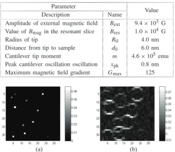
Fig. 1. Simulated true image and MRFM raw image exhibiting superposition of point responses (see Fig. 2) and noise. (a) Sparse true image (kxk0=11). (b) Raw MRFM observation.
by ensemble averages over the generated samples after the burn-in period. The joint MAP estimator is selected among the drawn samples, after the stationary distribution is achieved, such that it maximizes the posterior distribution f (x, λ|y) [31].
A. Simulation on Simulated Sparse Images
We performed simulations of MRFM measurements for PSF and image models similar to those described by Dobigeon et al. [12]. The signal-to-noise ratio was set to SNR = 10 dB. Several 32×32 synthetic sparse images, one of which is depicted in Fig. 1(a), were used to produce the data and were estimated using the proposed Bayesian method. The assumed PSF κ0 is generated following the physical model
described by Mamin et al. [13] when the physical parameters are tuned to the values displayed in Table I. This yields a 11 × 11 2-D convolution kernel represented in Fig. 2(a). We assume that the true PSF κ comes from the same physical model where the radius of the tip and the distance from the tip to the sample have been mis-specified with 2% error as
R = R0−2% = 3.92 and d = d0+2% = 6.12. This leads
to the convolution kernel depicted in Fig. 2(b). The observed measurements y, shown in Fig. 1(b), are a 32 × 32 image of size P = 1024.
The proposed algorithm requires the definition of K basis vectors vk, k = 1, . . . , K , that span a subspace representing
possible perturbations 1κ. We empirically determined this basis using the following PSF variational eigendecomposi-tion approach. A set of 5000 experimental PSFs ˜κj, j =
1, . . . , 5000, were generated following the model described by Mamin et al. [13] with parameters d and R randomly drawn according to Gaussian distribution1 centered at the
1We used a PSF generator provided by Dan Rugar’s group at IBM [13].
The variances of the Gaussian distributions are carefully tuned so that their standard deviations produce a minimal volume ellipsoid that contains the set of valid PSFs of the form specified in [13].
(a) (b)
Fig. 2. Assumed PSF κ0 and actual PSF κ. (a) Nominal MRFM PSF.
(b) True MRFM PSF.
Fig. 3. Scree plot of residual PCA approximation error in l2norm (magnitude
is normalized up to the largest value, i.e., λmax:=1).
nominal values d0, R0, respectively. Then a standard principal
component analysis (PCA) of the residuals { ˜κj−κ0}j =1,...,5000,
by allowing the maximum variance over the parameters that produce valid MRFM PSFs, was used to identify K = 4 principal axes that are associated with the basis vectors vk.
The necessary number of basis vectors, K = 4 here, was determined empirically by detecting a knee at the scree plot shown in Fig. 3. The first four eigenfunctions, corresponding to the first four largest eigenvalues, explain 98.69% of the observed perturbations. The four principal patterns of basis vectors are depicted in Fig. 4.
The proposed semi-blind Bayesian reconstruction algorithm was applied to estimate both the sparse image and the PSF coefficients of vk’s, using the prior in (6). From the
observa-tion shown in Fig. 1(b) the PSF estimated by the proposed algorithm is shown in Fig. 5(a) and is in good agreement with the true one. The corresponding maximum a posteriori estimate (MAP) of the unknown image is depicted in Fig. 6. The obtained coefficients of the PSF eigenfunctions are close to true coefficients (Fig. 7).
B. Comparison to Other Methods
For comparison to a nonblind method, Fig. 6(b) shows the estimate using the Bayesian nonblind method [12] with a mismatched PSF. Fig. 6(c) shows the estimate gener-ated by the AM algorithm. The nominal PSF described in Section V-A is used in the AM algorithm and hereafter
Fig. 4. K = 4 principal vectors (vk) of the perturbed PSF, identified
by PCA.
(c) (d)
(a) (b)
Fig. 5. Estimated PSF ˆκ of MRFM tip using our semi-blind method, Amizic’s method (using TV prior), Almeida’s method (using progressive regularization), and Tzikas’ method (using the kernel basis PSF model), respectively. For a fair comparison, we used sparse image priors for the methods. (See Section V-B for details on the methods.) (a) Proposed method. (b) Amizic’s method. (c) Almeida’s method. (d) Tzikas’ method.
in other semi-blind algorithms, and the parameter values of AM algorithm were set empirically according to the procedure in [24]. Our proposed algorithm appears to outperform the others (Fig. 6) while preserving fast convergence (Fig. 7).
Quantitative comparisons were obtained by generating dif-ferent noises in 100 independent trials for a fixed true image. Here, six different true images with six corresponding different sparsity levels (kxk0 = 6, 11, 18, 30, 59, 97) were
tested. Fig. 8 presents the two histograms of the results with the six sets in the corresponding two error criteria, kˆx − xk2, kˆxk0, respectively, both of which indicate that our
method performs better and is more stable than the other two methods.
Fig. 9 shows reconstruction error performance for sev-eral measures of error used by Ting et al. [11] and Dobigeon et al. [12] to compare different reconstruction algorithms for sparse MRFM images. Notably, compared
(a) (b)
(c) (d)
(e)
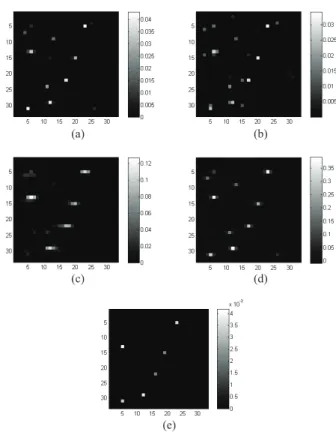
Fig. 6. True sparse image and estimated images from Bayesian nonblind, AM, our semi-blind, Almeida’s, and Tzikas’ methods. (a) MAP, proposed method. (b) MAP, Bayesian non blind method with κ0. (c) AM. (d) Almeida’s
method. (e) Tzikas’ method.
Fig. 7. Estimated PSF coefficients for four PCs over 200 iterations. These curves show fast convergence of our algorithm. “Ideal coefficients” are the projection values of the true PSF onto the space spanned by four principal PSF bases.
to the AM algorithm that aims to compensate “blindness” of the unknown PSF and the previous nonblind method, our method reveals a significant performance gain under most of the investigated performance criteria and sparsity conditions.
In addition to the AM and nonblind comparisons shown in Fig. 8, we made direct comparisons between our sparse MRFM reconstruction method and several state-of-the-art blind image reconstruction methods [22], [23], [25], [32], [33]. In all cases, the algorithms were initialized with the nominal, mismatched PSF and were applied to a sparse MRFM-type image like in Fig. 1. For a fair comparison, we made a sparse prior modification in the image model of other algorithms. The total variation (TV)-based prior for the PSF suggested by Amizic et al. [32] was also implemented. The obtained PSF from this method was considerably worse than the one
(a)
(b)
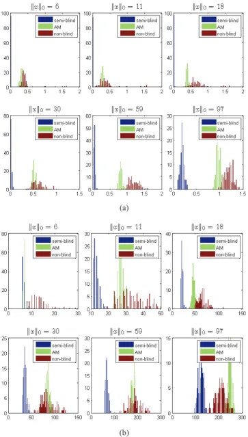
Fig. 8. Histograms of l2 and l0 norm of the reconstruction error. Note
that the proposed semi-blind reconstructions exhibit smaller mean error and more concentrated error distribution than the nonblind method in [12] and the AM method in [24]. (a) Histograms of the normalized l2 norm errors.
x-axis is k(x/kxk) − (ˆx/kˆxk)k22/kxk0. (b) Histograms of the l0 measures.
x-axis is kˆxk0.
estimated by our proposed method [see Fig. 5(b)] resulting in a very poor quality image deconvolution.2
The recent blind deconvolution method proposed by Almeida et al. [33] utilizes the “sharp Edge” property in natural images, with initial, high-regularization in order to effectively evaluate the PSF. This iterative approach has a sequentially decreasing regularization parameter to reconstruct fine details of the image. Adapted to sparse images, this method performs worse than our method, in terms of image and PSF estimation errors. The PSF and image estimates from Almeida’s method are presented in Figs. 5(c) and 6(d), respectively.
2Because this PSF is wrongly estimated and similar to the 2-D delta
func-tion, the image estimate looks similar to the denoised version of observafunc-tion, so we omit the image estimate.
(a) (b)
(c) (d)
Fig. 9. Error bar graphs of results from our myopic deconvolution algorithm. For several image xs of different sparsity levels, errors are illustrated with standard deviations. (Some of the sparsity measure and residual errors are too large to be plotted together with results from other algorithms.) (a) kˆxk0/kxk0:
estimated sparsity. Normalized true level is 1. (b) k(x/kxk)−(ˆx/kˆxk)k22/kxk0:
normalized error in reconstructed image. (c) ky − ˆyk2
2/kxk0: residual
(projection) error. (d) k( ˆκ/k ˆκk) − (κ/kκk)k22, as a performance gauge of our myopic method. At the initial stage of the algorithm, k(κ0/kκ0k) − (κ/kκk)k22=0.5627.
Tzikas et al. [25] use a similar PSF model to our method using basis kernels. However, no sparse image prior was assumed in [25] making it unsuitable for sparse reconstruction problems such as the MRFM problem considered in the paper. For a fair comparison, we applied the suggested PSF model [25] along with our sparse image prior. The results of PSF and image estimation and the performance graph are shown in Figs. 5(d), 6(e), and 9, respectively. In terms of PSF estimation error, our algorithm outperforms the others.
We also compared against the mixture model-based algo-rithm of Fergus et al. [22], and the related method of Shan et al. [23], which are proposed for blind deconvo-lution of shaking/motion blurs and do not incorporate any sparsity penalization. When applied to the sparse MRFM reconstruction problem, the algorithms in [22] and [23] per-formed very poorly (produced divergent or trivial solutions, not shown due to space limitations). This poor performance is likely due to the fact that the shape of the MRFM PSF and the sparse image model are significantly different from those in blind deconvolution of camera shaking/motion blurs. The generalized PSF model in [22] and [23] with the sparse image prior is Tzikas’ model [25], which is described above.
We used the iterative shrinkage/thresholding (IST) algorithm with a true PSF to lower bound our myopic reconstruction algorithm. The IST algorithm effectively
TABLE II
COMPUTATIONTIME OFALGORITHMS(INSECONDS), FOR THEDATA INFIG. 1
Proposed method 19.06 Bayesian nonblind [12] 3.61 IST [34] 0.09 AM [24] 0.40 Almeida’s method [33] 5.63 Amizic’s method [32] 5.69 Tzikas’ method [25] 20.31
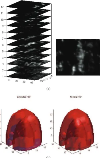
Fig. 10. Observed data at various tip-sample distances z.
reconstructs images with a sparsity constraint [34]. From Fig. 9(b) the performance of our result is as good as that of the oracle IST. In Table II, we present comparison of computation time3 of the proposed sparse semi-blind Bayes
reconstruction to that of several other algorithms.
C. Application to 3-D MRFM Image Reconstruction
In this section, we apply the semi-blind Bayesian recon-struction algorithm to the 3-D MRFM tobacco virus data [6] shown in Fig. 10. The necessary modification for our algorithm to apply to 3-D data is simple because the extension of our 2-D pixel-wise sampling method requires only one more added dimension to extend to 3-D basis vectors and 3-D convolution kernel. As seen in Appendix A, the voxel-wise update of a vectorized image x can be generalized to n-D data. This scalability is another benefit of our algorithm. The implementation of the AM algorithm is impractical due to its slow convergence rates [24]. Here, we only consider Bayesian methods. The additive noise is assumed Gaussian consis-tently with [4] and [6], so the noise model in Section III-A is applied here.
The PSF basis vectors were obtained from a standard PCA and the number of principal components in the PSF perturbation was selected as 4 based on detecting the knee in a scree plot. The same interpolation method as used in [12] was adopted to account for unequal spatial sampling rates in the supplied data for the PSF domain and the image domain. In the PSF and image domains, along the z-axis, the grid in PSF signal space is three times finer than the observation sampling density, because the PSF sampling rate along the
z-axis is three times higher than the data sampling rate. To
interpolate this lower sampled data, we implemented a version of the Bayes MC reconstruction that compensates for unequal projection sampling in the z-directions using the interpolation procedure of Dobigeon et al. [12].
3MATLAB is used under Windows 7 Enterprise and HP-Z200 (Quad
2.66 GHz) platform.
(a) (b)
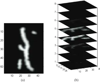
Fig. 11. Results of applying the proposed semi-blind sparse image recon-struction algorithm to the synthetic 3-D MRFM virus image. (a) Ground truth synthetic virus image obtained from data by Degen et al. [6]. (b) Semi-blind reconstruction of the synthetic virus data. Only the z-planes that have nonzero image intensity are shown.
(c)
(a) (b)
Fig. 12. PSF estimation result. (a) True PSF. (b) Initial mismatched PSF. (c) Estimated PSF.
To demonstrate that the proposed 3-D MCMC semi-blind reconstruction algorithm is capable of reconstruction in the presence of significant MRFM PSF mismatch, we first applied it to a simulated version of the experimental data shown in Fig. 10. We used the scanning electron microscope virus image reported by Degen et al. [6] to create a synthetic 3-D MRFM virus image, one slice of which is shown in Fig. 11(a). This 3-D image was then passed through the MRFM forward model, shown in Fig. 12(a), and 10 dB Gaussian noise was added. The mismatched PSF depicted in Fig. 12(b) was used to initialize our proposed semi-blind reconstruction algorithm. After 40 iterations, the algorithm reduced the initial normalized PSF error k(κ0/kκ0k) − (κ/kκk)k2 from 0.7611 to k( ˆκ/k ˆκk) −
(κ/kκ k)k2=0.0295. Figs. 11(b) and 12(c) show the estimated image and the estimated PSF, respectively.
We next applied the proposed semi-blind reconstruction algorithm to the actual experimental data shown in Fig. 10 for which there is neither ground truth on the MRFM image
(a)
(b)
Fig. 13. Semi-blind MC Bayes method results and PSF coefficient curves. 1z =4.3 nm, and pixel spacing is 8.3 nm × 16.6 nm in x × y, respectively. The size of (x, y) plane is 498 nm × 531.2 nm. Smoothing is applied for visualization. (a) MAP estimate in 3-D and the estimated image on the sixth plane, showing a virus particle. (b) Estimated (left) and nominal (right) PSFs. k( ˆκ/k ˆκk) − (κ0/kκ0k)k2 =0.0212. The difference between the two is small. (Hard thresholding with level = max(P S F) × 10−4 is applied for
visualization.)
nor on the MRFM PSF. The image reconstruction results are shown in Fig. 13. The small difference between the nominal PSF and the estimated PSF indicates that the estimated PSF is close to the assumed PSF. We empirically validated this small difference by verifying that multiple runs of the Gibbs sampler gave low variance PSF residual coefficients. We conclude from this finding that the PSF model of Degen et al. [6] is in fact nearly Bayes optimal for these experimental data. The blind image reconstruction shown in Fig. 13 is similar to the image reconstruction in Degen et al. [6] obtained from applying the Landweber reconstruction algorithm with the nominal PSF.
Using the MCMC generated posterior distribution obtained from the experimental MRFM data, we generated confidence intervals, posterior mean, and posterior variance of the pixel intensities of the unknown virus image. The posterior mean and variance are presented in Fig. 14 for selected pixels. In addition, to demonstrate the match between the estimated region occupied by the virus particle and the actual region, we evaluated Bayesian p-values for object regions. The
(a) (b)
Fig. 14. Posterior mean and variance at the sixth plane of the estimated image, as shown in Fig. 13(a). (a) MMSE solution. Gray level image intensity values range from 0 (black) to 7.34 × 10⁻¹² (white). (b) Pixel-wise square root of the image variance. White color indicates a high-variance. Gray level image intensity values range from 0 (black) to 3.29 × 10⁻¹²(white).
Bayesian p-value for a specific region Ri having nonzero
intensity is pv(Ri) = P({Ik = 1}k∈Ri|y) where P is a
probability measure and Ik is an indicator function at the kth
voxel. Assuming voxel-wise independence, the p-values are easily computed from the posterior distribution and provide a level of a posteriori confidence in the statistical significance of the reconstruction. We found that over 95% of the Bayesian p-values were greater than 0.5 for the nonzero regions of the reconstruction.
D. Discussion
Joint identifiability is a common issue underlying all blind deconvolution methods. (e.g., scale ambiguity.) Even though the unicity of our solution is not proven, given the conditions that: 1) span(κ) = κ0+span(4κi)does not cover a kernel of
a delta function, κ = δ(·) and 2) the PSF solution is restricted to this linear space of κ0, κi, the MAP estimate computed from
(17) is a reasonable solution that is not trivial the MAP criteria promises a reasonable solution that is not trivial such as ˆx = y. Due to this restriction and the sparse nature of the image to be estimated, we can reasonably expect that the solution provided by the algorithm is close to the true PSF. A study of unicity of the solution would be worthwhile but is beyond the scope of this paper as it would require study of the complicated and implicit fixed points of the proposed Bayes objective function. Note that proposed sparse image reconstruction algorithm can be extended to exploit sparsity in other domains, such as the wavelet domain. In this case, if we define W to be the transformation matrix on x, the proposed semi-blind approach can be applied to reconstruct the transformed signal z = Wx. However, instead of assigning the single-sided exponential dis-tribution as prior for z, a double-sided Laplacian disdis-tribution might be used to cover the negative values of the pixels. The estimation procedure for PSF coefficients, noise level, and hyperparameters would be the same. For image estimation, the vector hi used in (22) would be replaced with the ith column
of HW−1.
VI. CONCLUSION
We have proposed an extension of the method of the nonblind Bayes reconstruction by Dobigeon et al. [12] that simultaneously estimates a partially known PSF and the unknown but sparse image. The method uses a prior model on the PSF that reflects a nominal PSF and uncertainty about
the nominal PSF. In our algorithm, the values of the parameters of the convolution kernel were estimated by a Metropolis-within-Gibbs algorithm, with an adaptive mechanism for tun-ing random-walk step size for fast convergence. Our approach can be used to empirically evaluate the accuracy of assumed nominal PSF models in the presence of model uncertainty. In our sparse reconstruction simulations, we demonstrated that the semi-blind Bayesian algorithm has improved performance as compared to the AM reconstruction and other blind decon-volution algorithms and nonblind Bayes method under several criteria.
Possible extensions of the proposed method may include enforcing sparsity constraints on the result PSF and the eigenfunctions, by using sparse PCA type algorithms. Also, even with the selective sampling strategy that speeds up the sampling, the MCMC methods are slower than nonstochastic methods. This will be addressed in future work.
APPENDIXA
FASTRECURSIVESAMPLINGSTRATEGY
In iterative MRFM algorithms such as AM and the proposed Bayesian method, repeated evaluations of the transformation
T(κ (λ) , x) can be computationally difficult. For example, at each iteration of the proposed Bayesian myopic deconvolution algorithm, one must generate xi from its conditional
distrib-ution f (xi|w, a, λ,σ2, x−i, y), which requires the calculation
of T (κ, ˜xi) where ˜xi is the vector x whose ith element has
been replaced by 0. Moreover, sampling according to the conditional posterior distributions of σ2and λk (23) and (26)
requires computations of T (κ, x).
By exploiting the bilinearity of the transformation T (·, ·), we can reduce the complexity of the algorithm. We describe below a strategy, similar to those presented in [12, Appendix B], which only requires computation of T (·, ·) at most M × (K + 1) times. First, let IM denote the M × M
identity matrix and ui its ith column. In the first step of the
analysis, the M vectors h(0)i (i = 1, . . . , M)
h(0)i = T (κ0, ui) (27)
and KM vectors h(k)
i (i = 1, . . . , M, k = 1, . . . , K )
hi(k)= T (vk, ui) (28)
are computed. Then one can compute the quantity T (κ, ˜xi)
and T (κ, x) at any stage of the Gibbs sampler without evaluating T (·, ·), based on the following decomposition:
T(κ, x) = M ! i=1 xih(0)i + K ! k=1 λk M ! i=1 xih(k)i . (29)
The resulting procedure to update the ith coordinate of the vector x is described in Algorithm 3.
Note that in step 7 of the algorithm above, T (κ, x) is recur-sively computed. Once all the coordinates have been updated, the current T (κ, x) can be directly used to sample according to the posterior distribution of the noise variance in (26). Moreover, this quantity can be used to sample according to the conditional posterior distribution of λkin (23). More precisely,
Algorithm 3 Efficient Simulation According to
f(x|w, a, σ2, y)
At iteration t of the Gibbs sampler, for i = 1, . . . , M, update the ith coordinate of the vector
x(t,i−1)=*x1(t ), . . . , xi−(t )1, xi(t −1), xi+(t −1)1 , . . . , x(t −1)M +T via the following steps:
1: compute hi = h(0)i +
4K
k=1λkh(k)i ,
2: set T"κ, ˜x(t,i−1)i #= T.κ, x(t,i−1)/− xi(t −1)hi,
3: set ei = x − T
"
κ, ˜x(t,i−1)i #,
4: compute µi, η2i and wi as defined in [6],
5: draw xi(t ) according to (21), 6: set x(t,i)=*x(t ) 1 , . . . , xi−(t )1, xi(t ), x (t −1) i+1 , . . . , x(t −1)M +T ,
7: set T.κ, x(t,i)/= T"κ, ˜x(t,i−1)i #+ x(t )i hi.
evaluating T.κ.λ⋆k/, x/in the acceptance probability (25) can be recursively evaluated as follows:
T .κ.λ⋆k/, x/= T"κ"λ(t )k #, x#−"λ(t )k − λ⋆k# M ! i=1 xihi(k). (30) APPENDIXB
SPARSITYENFORCINGSELECTIVESAMPLING
Since we have estimated the “overall sparsity,” 1 − ˆwof x from (19), we can expedite the sampling procedure of x by selectively sampling only significant portions of entire pixels of x. As a result, we expect (1 − ˆw) ×100% of pixel domain of x to be zero, which will not need to be resampled.
At time t, in order to approximate the quantile (1 − ˆw)of {w(t )i }i=1,...,M in (21) we evaluate the (1− ˆw)quantile value of
the previously obtained {wi(t −1)}i=1,...,M. This approximation
accelerates the computation because the exact calculation of {w(t )
i }i=1,...,M requires sampling of all xis. Let q =
quantile({w(t −1)i }i=1,...,M,1 − ˆw) and wthr =max(q, 1 − ˆw).
When w(t )
i for x
(t )
i from (21) is less than wthr, then x
(t )
i is
not updated or is set to zero. Because MCMC sampling is computationally expensive, especially for large size images, this suggestion can be restricted to the burn-in period to save computations.
In our experiment, the selective sampling of x applied after third or fourth iterations produces equally good results compared to the conventional MCMC sampling methods, while reducing computation time by 30%–50% for nonblind sparse reconstruction with a fixed PSF and by 10%–30% for the semi-blind sparse reconstruction.
APPENDIXC
ADAPTIVETUNING OF ANACCEPTANCERATE IN THERANDOM-WALKSAMPLING
For an efficient sampling of λk, k = 1, . . . , K, from the
Algorithm 4Tuning s in the Gaussian Proposal Density q(·, ·)
Select upper and lower limits accH and accL. At each
time t = W,2W, 3W, . . ., tune s via the following steps:
1: Evaluate accs using (31) for the given time-frame window,
2: Update s ← s × c,if accs >accH, s ÷ c,if accs <accL, s, otherwise.
properly tune the acceptance rate of the samples from the proposal distribution. A careful selection of a step size is critical for convergence of the method. For example, if the step size is too large, most of the iterations will be rejected and the sampling algorithm will be inefficient. On the other hand, if the step size is too small, most of the random walk moves are accepted but these moves are slow to cover the probable space of the desired distribution, and the method is once again inefficient.
The transition density of Metropolis–Hastings sampling is q(λ(t ), λ⋆(t ))acc(λ(t ), λ⋆(t )), where q(λ(t ), λ⋆(t )) is the
proposal density from λ(t )and acc(λ(t ), λ⋆(t ))is the acceptance
probability for the move from λ(t )to λ⋆(t ). Here, we denote λ
k
by λ without a subscript for simplicity. We set q(λ(t ), λ⋆(t ))
to be a Gaussian density function of λ⋆(t ), denoted by q(λ(t ), λ⋆(t )) = q(λ⋆(t ) − λ(t )) = φ(λ⋆(t ); λ(t ), s2) with a mean λ(t ) and a variance s2, which produces a random walk
sample path. Since q(·, ·) is symmetrical, accs(λ(t ), λ⋆(t )) =
min(1, (π(λ⋆(t ))q(λ⋆(t ), λ(t ))/π(λ(t ))q(λ(t ), λ⋆(t )))) = min
(1, (π(λ⋆(t ))/π(λ(t )))) = ρ
λ(t)→λ⋆(t), as derived in (24). Then
the acceptance probability from a parameter value λ(t ) is
accs(λ(t )) =
8
λ⋆(t)q(λ(t ), λ⋆(t ))accs(λ(t ), λ⋆(t ))dλ⋆(t ). The
acceptance rate with a scale parameter s, acting as a step size, can be expressed as accs =
8
λπ(λ)accs(λ)dλ.
We evaluate these integrations by using Monte Carlo meth-ods, accs ≈ (1/n1)4nt =11accs(λ(t ))with λ(t ) ∼ π(λ(t )), and
accs(λ(t )) ≈ (1/n2)4nt =21accs(λ(t ), λ⋆(t ))with λ⋆(t )∼ q(λ(t ),
λ⋆(t )). In practice, this empirical version of the integration value is evaluated as accs ≈ 1 W W ! t =1 accs " λ(t )λ⋆(t )# (31)
after the burn-in period. Therefore, we can evaluate the acceptance rate with s by averaging the Boolean variables of accs(λ(t ), λ⋆(t )), t =1, . . . , W , over a time-frame window of
length W with realizations {λ(t ), λ⋆(t )}
t. In short, we iteratively
update s to achieve an appropriate acceptance rate accs as
described in Algorithm 4.
In practice, we fix the variance of the instrumental distribu-tion at the end of a burn-in period. Consequently, the transidistribu-tion kernel will be fixed and this guarantees both ergodicity and stationary distribution. In our experiment, we set a conser-vative acceptance range, accH = 0.6, accL = 0.4, referring
to [29], and W = 20, c = 4. This strategy can also be applied to the direct parameter estimation described in Appendix D.
APPENDIXD
DIRECTSAMPLING OFPSF PARAMETERVALUES
As described in Section I, in the MRFM experiments, the direct estimation of PSF parameters is difficult because of the nonlinearity of κgen and the slow evaluation of κgen(ζ′)
given a candidate value ζ′. However, if κ
gen is simple and
evaluated quickly, then a direct sampling of parameter values can be performed. To apply this sampling method, instead of calculating a linearized convolution kernel κ (λ), we evaluate the exact model PSF, κgen(ζ ), in (23) and (25). Also, the proposed parameter vector ζ⋆correspondingly replaces a
coef-ficient vector λ⋆ and the updated PSF is used in the estimation
of other variables. This strategy turns out to be similar to the approach adopted by Orieux et al. [26].
ACKNOWLEDGMENT
The authors would like to thank D. Rugar for providing the tobacco virus data and insightful comments on this paper. They would also like to thank the reviewers for their comments, which helped the authors significantly improve the quality of this paper.
REFERENCES
[1] J. A. Sidles, “Noninductive detection of single-proton magnetic reso-nance,” Appl. Phys. Lett., vol. 58, no. 24, pp. 2854–2856, Jun. 1991. [2] J. A. Sidles, “Folded Stern-Gerlach experiment as a means for detecting
nuclear magnetic resonance in individual nuclei,” Phys. Rev. Lett., vol. 68, no. 8, pp. 1124–1127, Feb. 1992.
[3] J. A. Sidles, J. L. Garbini, K. J. Bruland, D. Rugar, O. Züger, S. Hoen, and C. S. Yannoni, “Magnetic resonance force microscopy,” Rev. Mod.
Phys., vol. 67, no. 1, pp. 249–265, Jan. 1995.
[4] D. Rugar, C. S. Yannoni, and J. A. Sidles, “Mechanical detection of magnetic resonance,” Nature, vol. 360, no. 6404, pp. 563–566, Dec. 1992.
[5] O. Züger, S. T. Hoen, C. S. Yannoni, and D. Rugar, “Three-dimensional imaging with a nuclear magnetic resonance force microscope,” J. Appl.
Phys., vol. 79, no. 4, pp. 1881–1884, Feb. 1996.
[6] C. L. Degen, M. Poggio, H. J. Mamin, C. T. Rettner, and D. Rugar, “Nanoscale magnetic resonance imaging,” Proc. Nat. Acad. Sci., vol. 106, no. 5, pp. 1313–1317, Feb. 2009.
[7] S. Chao, W. M. Dougherty, J. L. Garbini, and J. A. Sidles, “Nanometer-scale magnetic resonance imaging,” Rev. Sci. Instrum., vol. 75, no. 5, pp. 1175–1181, Apr. 2004.
[8] O. Züger and D. Rugar, “First images from a magnetic resonance force microscope,” Appl. Phys. Lett., vol. 63, no. 18, pp. 2496–2498, 1993. [9] O. Züger and D. Rugar, “Magnetic resonance detection and imaging
using force microscope techniques,” J. Appl. Phys., vol. 75, no. 10, pp. 6211–6216, May 1994.
[10] C. L. Degen, M. Poggio, H. J. Mamin, C. T. Rettner, and D. Rugar, “Nanoscale magnetic resonance imaging,” Proc. Nat. Acad. Sci., vol. 106, no. 5, pp. 1–5, Feb. 2009.
[11] M. Ting, R. Raich, and A. O. Hero, “Sparse image reconstruction for molecular imaging,” IEEE Trans. Image Process., vol. 18, no. 6, pp. 1215–1227, Jun. 2009.
[12] N. Dobigeon, A. O. Hero, and J.-Y. Tourneret, “Hierarchical Bayesian sparse image reconstruction with application to MRFM,” IEEE Trans.
Image Process., vol. 18, no. 9, pp. 2059–2070, Sep. 2009.
[13] J. Mamin, R. Budakian, and D. Rugar, “Point response function of an MRFM tip,” IBM Research Division, Rueschlikon, Switzerland, Tech. Rep., Oct. 2003.
[14] S. Makni, P. Ciuciu, J. Idier, and J.-B. Poline, “Semi-blind deconvolution of neural impulse response in fMRI using a Gibbs sampling method,” in Proc. IEEE Int. Conf. Acoust., Speech, Signal, vol. 5. May 2004, pp. 601–604.
[15] G. Pillonetto and C. Cobelli, “Identifiability of the stochastic semi-blind deconvolution problem for a class of time-invariant linear systems,”
[16] P. Sarri, G. Thomas, E. Sekko, and P. Neveux, “Myopic deconvolution combining Kalman filter and tracking control,” in Proc. IEEE Int. Conf.
Acoust., Speech, Signal, vol. 3. May 1998, pp. 1833–1836.
[17] G. Chenegros, L. M. Mugnier, F. Lacombe, and M. Glanc, “3D phase diversity: A myopic deconvolution method for short-exposure images: Application to retinal imaging,” J. Opt. Soc. Amer. A, vol. 24, no. 5, pp. 1349–1357, May 2007.
[18] R. Molina, “On the hierarchical Bayesian approach to image restoration: Applications to astronomical images,” IEEE Trans. Pattern Anal. Mach.
Intell., vol. 16, no. 11, pp. 1122–1128, Nov. 1994.
[19] N. P. Galatsanos, V. Z. Mesarovic, R. Molina, and A. K. Katsaggelos, “Hierarchical Bayesian image restoration from partially known blurs,”
IEEE Trans. Image Process., vol. 9, no. 10, pp. 1784–1797, Oct. 2000. [20] N. P. Galatsanos, V. Z. Mesarovic, R. Molina, A. K. Katsaggelos, and J. Mateos, “Hyperparameter estimation in image restoration problems with partially known blurs,” Opt. Eng., vol. 41, no. 8, pp. 1845–1854, 2002.
[21] R. Molina, J. Mateos, and A. K. Katsaggelos, “Blind deconvolution using a variational approach to parameter, image, and blur estimation,”
IEEE Trans. Image Process., vol. 15, no. 12, pp. 3715–3727, Dec. 2006.
[22] R. Fergus, B. Singh, A. Hertzmann, S. T. Roweis, and W. T. Freeman, “Removing camera shake from a single photograph,” in Proc. ACM
SIGGRAPH Papers, 2006, pp. 787–794.
[23] Q. Shan, J. Jia, and A. Agarwala, “High-quality motion deblurring from a single image,” ACM Trans. Graph., vol. 27, no. 3, p. 1, 2008. [24] K. Herrity, R. Raich, and A. O. Hero, “Blind reconstruction of sparse
images with unknown point spread function,” Proc. SPIE Comput.
Imaging, vol. 6814, no. 1, pp. 68140K-1–68140K-11, Jan. 2008. [25] D. Tzikas, A. Likas, and N. Galatsanos, “Variational Bayesian sparse
kernel-based blind image deconvolution with Student’s-t priors,” IEEE
Trans. Image Process., vol. 18, no. 4, pp. 753–764, Apr. 2009.
[26] F. Orieux, J.-F. Giovannelli, and T. Rodet, “Bayesian estimation of regularization and point spread function parameters for Wiener-Hunt deconvolution,” J. Opt. Soc. Amer. A, vol. 27, no. 7, pp. 1593–1607, Jul. 2010.
[27] T. Hastie, R. Tibshirani, and J. Friedman, The Elements of Statistical
Learning: Data Mining, Inference, and Prediction. New York: Springer-Verlag, Aug. 2003.
[28] M. Ting, R. Raich, and A. O. Hero, “Sparse image reconstruction using sparse priors,” in Proc. IEEE Int. Conf. Image Process., Oct. 2006, pp. 1261–1264.
[29] C. P. Robert and G. Casella, Monte Carlo Statistical Methods. New York: Springer-Verlag, 1999.
[30] P. Bremaud, Markov Chains: Gibbs Fields, Monte Carlo Simulation, and
Queues. New York: Springer-Verlag, 1999.
[31] J.-M. Marin and C. P. Robert, Bayesian Core: A Practical Approach to
Computational Bayesian Statistics. New York: Springer-Verlag, 2007.
[32] B. Amizic, S. D. Babacan, R. Molina, and A. K. Katsaggelos, “Sparse Bayesian blind image deconvolution with parameter estimation,” in Proc.
Eur. Signal Process. Conf.. Aalborg, Denmark, Aug. 2010, pp. 626–630. [33] M. Almeida and L. Almeida, “Blind and semi-blind deblurring of natural images,” IEEE Trans. Image Process., vol. 19, no. 1, pp. 36–52, Jan. 2010.
[34] I. Daubechies, M. Defrise, and C. De Mol, “An iterative thresholding algorithm for linear inverse problems with a sparsity constraint,”
Com-mun. Pure Appl. Math., vol. 57, no. 11, pp. 1413–1457, 2004.
Se Un Park received the B.S. degree in electrical engineering from the Korea Advanced Institute of Science and Technology, Daejeon, Korea, in 2004, and the M.S. and M.A. degrees in electrical engi-neering and statistics from the University of Michi-gan, Ann Arbor, in 2009 and 2011, respectively, where he is currently pursuing the Ph.D. degree in electrical engineering.
His current research interests include statistical signal processing, image processing, and machine learning.
Nicolas Dobigeon (S’05–M’08) was born in Angoulême, France, in 1981. He received the Eng. degree in electrical engineering from École Nationale Supérieure d’Électronique, d’Électrotechnique, d’Informatique, d’Hydraulique et des Télécommunications (ENSEEIHT), Toulouse, France, and the M.Sc. and Ph.D. degrees in signal processing from the National Polytechnic Institute of Toulouse, Toulouse, in 2004, 2004, and 2007, respectively.
He was a Post-Doctoral Research Associate with the Department of Electrical Engineering and Computer Science, University of Michigan, Ann Arbor, from 2007 to 2008. Since 2008, he has been an Assistant Professor with ENSEEIHT, National Polytechnic Institute of Toulouse, University of Toulouse, Toulouse, and with the Signal and Communication Group, IRIT Laboratory, Toulouse. His current research interests include statistical signal and image processing with a particular interest in Bayesian inference and Markov chain Monte Carlo methods.
Alfred O. Hero(S’79–M’84–SM’96–F’98) received the B.S. (summa cum laude) degree from Boston University, Boston, MA, and the Ph.D. degree from Princeton University, Princeton, NJ, in 1980 and 1984, respectively, both in electrical engineering.
He has been with the University of Michigan, Ann Arbor, since 1984, where he is the R. Jamison and B. Williams Professor of engineering. His pri-mary appointment is with the Department of Elec-trical Engineering and Computer Science, and he has appointments with the Department of Biomedical Engineering and the Department of Statistics. He has held visiting positions with the Laboratory for Information and Decision Systems, Massachusetts Institute of Technology, Cambridge, in 2006, Boston University in 2006, I3S University of Nice, Sophia-Antipolis, France, in 2001, École Normale Supérieure de Lyon, Lyon, France, in 1999, École Nationale Supérieure des Télécom-munications, Paris, France, in 1999, Lucent Bell Laboratories, Murray Hill, NJ, in 1999, Scientific Research Laboratory, Ford Motor Com-pany, Dearborn, MI, in 1993, École Nationale Supérieure des Tech-niques Avancees, École Supérieure d’Electricite, Paris, in 1990, and M.I.T. Lincoln Laboratory, Cambridge, from 1987 to 1989. His current research interests include detection, classification, pattern analysis, adap-tive sampling for spatiotemporal data, applications to network security, multimodal sensing and tracking, biomedical imaging, and genomic signal processing.
Dr. Hero was a recipient of the Digiteo Chaire d’Excellence from Digiteo Research Park, École Supérieure d’Electricite, France, and the University of Michigan Distinguished Faculty Achievement Award in 2011. He received several Best Paper Awards, including the IEEE Signal Processing Society Best Paper Award in 1998, the Best Original Paper Award from the Journal of Flow Cytometry in 2008, and the Best Magazine Paper Award from the IEEE Signal Processing Society in 2010. He received the IEEE Signal Processing Society Meritorious Service Award in 1998, the IEEE Third Millennium Medal in 2000, and the IEEE Signal Processing Society Distinguished Lecturership in 2002. He has been a plenary and keynote speaker at major workshops and conferences. He was the President of the IEEE Signal Processing Society from 2006 to 2007. He was on the Board of Directors of the IEEE from 2009 to 2011, where he served as the Director Division IX of signals and applications.