Accuracy assessment of blind and semi-blind restoration methods for hyperspectral images

HAL Id: hal-01484534

https://hal-univ-rennes1.archives-ouvertes.fr/hal-01484534

Submitted on 2 Nov 2020

HAL is a multi-disciplinary open access

archive for the deposit and dissemination of

sci-entific research documents, whether they are

pub-lished or not. The documents may come from

teaching and research institutions in France or

abroad, or from public or private research centers.

L’archive ouverte pluridisciplinaire HAL, est

destinée au dépôt et à la diffusion de documents

scientifiques de niveau recherche, publiés ou non,

émanant des établissements d’enseignement et de

recherche français ou étrangers, des laboratoires

publics ou privés.

Accuracy assessment of blind and semi-blind restoration

methods for hyperspectral images

M. Zhang, B. Vozel, K. Chehdi, M. Uss, S. Abramov, V. Lukin

To cite this version:

M. Zhang, B. Vozel, K. Chehdi, M. Uss, S. Abramov, et al.. Accuracy assessment of blind and

semi-blind restoration methods for hyperspectral images. Image and Signal Processing for Remote Sensing

XXII, Sep 2016, Edinburgh, United Kingdom. �10.1117/12.2240950�. �hal-01484534�

Accuracy assessment of blind and semi-blind restoration methods for

hyperspectral images

Mo Zhang

, Benoit Vozel

, Kacem Chehdi

, Mykhail Uss

, Sergey Abramov

, Vladimir Lukin

_{University of Rennes 1, IETR UMR CNRS 6164, TSI2M, 22305 Lannion Cedex, France}

b

_{National Aerospace University, 61070, Kharkov, Ukraine}

ABSTRACT

Hyperspectral images acquired by remote sensing systems are generally degraded by noise and can be sometimes more severely degraded by blur. When no knowledge is available about the degradations present or the original image, blind restoration methods must be considered. Otherwise, when a partial information is needed, semi-blind restoration methods can be considered. Numerous semi-blind and quite advanced methods are available in the literature. So to get better insights and feedback on the applicability and potential efficiency of a representative set of four semi-blind methods recently proposed, we have performed a comparative study of these methods in objective terms of blur filter and original image error estimation accuracy. In particular, we have paid special attention to the accurate recovering in the spectral dimension of original spectral signatures. We have analyzed peculiarities and factors restricting the applicability of these methods. Our tests are performed on a synthetic hyperspectral image, degraded with various synthetic blurs (out-of-focus, gaussian, motion) and with signal independent noise of typical levels such as those encountered in real hyperspectral images. This synthetic image has been built from various samples from classified areas of a real-life hyperspectral image, in order to benefit from realistic reference spectral signatures to recover after synthetic degradation. Conclusions, practical recommendations and perspectives are drawn from the results experimentally obtained.

Keywords: remote sensing images, additive noise, semi-blind image restoration, sparse distribution, alternating minimization, regularization parameter, augmented Lagrangian, alternating direction method of multipliers (ADMM), total variation, stopping criteria.

1. INTRODUCTION

Based on an observed image at hand alone, the exceptionally challenging goal of blind or semi-blind image restoration is to combine at best (e.g. optimally with respect to a chosen estimation error criterion) the efficient estimation of both the original image and the whole set of degradations. This problem is required when the original image has suffered from degradations at the output of the imaging system with which the observed image was acquired. In such a framework, a standard model usually accepted to describe this observed image sufficiently well is the following: the observed image is assumed degraded by a blur with an observation noise. Both terms are considered with the goal to correctly model the contribution of each degradation source that possibly occurred at acquisition time. Recall that in the true blind case, no priors about the original image or its content (homogeneous area(s), texture(s), edge(s), contour(s)) and the degradations present (blur(s), noise(s)) are available at all, making the problem to solve hardly tractable. But in the semi-blind case, partial information on these unknowns or such as specific values of regularization parameters can be introduced. In practice, to partly alleviate the difficulties inherent to the restoration problem, the blur is generally modeled by a linear shift-invariant PSF (Point Spread Function) with an upper bound of its support in both spatial directions while the overall contribution of noise components can be assumed additive.

In particular, both aforementioned properties are often considered for hyperspectral images such as those acquired by last generation multichannel (multi or hyperspectral) remote sensing systems (mounted on satellite, airborne or UAV

platforms). These hyperspectral images are unavoidably degraded by noise(s) and can be sometimes more severely degraded by blur(s). Indeed, the hyperspectral image components (or spectral channels) may have suffered in varying proportion different blurring sources that can originate from either lens imperfections, defocusing, chromatic aberration, atmospheric or air turbulence, sensor-scene motion or from sensor drift and/or failure after the platform deployment. Note that the PSF shift-invariance is a property imposed on the resulting blur in each image component to simplify the problem compared to the more general PSF shift-variance case, although a few methods have been recently proposed to deal with this more complex latter case (see [1] and references therein). The contribution of noise in image components can be modeled as a mixture of additive and quasi-Poisson noise [2]. The relative weight of each term in such a mixed noise mainly depends on the sensor used and the actual conditions at the acquisition time.

As recalled previously, the blind or semi-blind restoration of such real-life degraded hyperspectral images addresses the estimation problem of the original image component in each spectral channel, based on the quite very restrictive set of above mentioned hypotheses (shift invariance of the PSF and the parameters of the mixed noise in each image component as well as given upper limit of the PSF extent in the two spatial directions). Another feature of hyperspectral images worth reminding at this stage is that the signal and noise levels as well as the resulting signal-to-noise ratio are known to vary in rather wide limits along the spectral dimension (in component images). Consequently, at the output of the processing performed, the overall spectral signature has to be recovered in each spatial position, and this should be achieved only resorting on the processing of the observed component images at hand and using specific regularization methods to compensate for missing information. An additional feature to keep in mind is that due to the large number of spectral channels that may reach several hundred for modern remote sensing systems, leading thus to a large amount of image components to restore in a blind or semi-blind manner, fully automatic, efficient and rather fast methods are of particular practical interest here.

However, the blind or semi-blind image restoration problem of monocomponent images, degraded in a manner similar to the one stated above for hyperspectral component images, is known to be a severely ill-posed problem. The main reason for this is that an infinite number of combinations of a PSF and an original image can give rise to the same observed image in the usual mean squared error sense. That is why blind and semi-blind methods generally introduce several regularization terms in the criterion they seek to optimize (most often to minimize) with the goal to replace the initial ill-posed problem by a well ill-posed problem. This amounts to impose additional constraints on the characteristics of the estimated PSF and/or original image. In practice, this results in additional regularization terms added to the basic a posteriori least-squares data fidelity criterion, each of them weighted by an associated regularization parameter to tune its relative strength in the overall objective function to optimize. The goal is to get the closest approximation of the true solution to the initial problem while ensuring facilitated convergence of the regularized restoration method and the compromise often met in practice is to be satisfied with an acceptable approximation to the true unknown solution.

The scientific literature focusing on image restoration is quite vast and numerous methods have been proposed. Some of these methods when finely tuned in their optimal operation point are able to get quite impressive results according to well-known standard assessment criteria such as the mean squared error (MSE) or the increase in signal to noise ratio (ISNR). The ISNR criterion is defined as the difference in decibels between the improved signal to noise ratio (SNR) obtained after restoration and the original SNR. But several drawbacks linked to still unresolved problems can be underlined as well. Among them, we can mention the difficulty to formalize adequate regularization terms. These terms have to be derived with respect to expected characteristics for solutions sought on one hand and convergence requirements on the other hand. This may results in possible instability of the derived method, convergence to local minima when convexity property of the resulting objective function is not guaranteed. Manual or non-automatic tuning of the optimal value of involved regularization parameters, sensitivity to initialization choice for different variables of interest (original image, PSF), heavy computational cost may be encountered as well.

In this paper, we are essentially interested in the ability and applicability of semi-blind restoration methods to operate automatically, efficiently and fast for the deconvolution of hyperspectral image components. In most cases, methods proposed as blind ones in the literature are rather semi-blind as they still resort to a minimum of a priori information. That is why we have retained in our study a representative set of four recently proposed methods [3-6]. All these methods consider either mono- or multi- component image and/or blur filter edge-sparsifying regularizers in order to favor images with sparse edges, aligned restored channels [3,4,6]. They can add specific constraints on the blur filter (sum-to-1 and non-negativity) as well [5,6]. They all carry out alternate minimization of the resulting multi-term cost

function with respect to the unknown image and the unknown blur (assumed spatially invariant), using possibly coarse to fine pyramid of image resolution approach. Based on the PSF estimated in the first alternate stage, the last two methods [5,6] apply a semi-blind deconvolution method for estimating the unknown image.

The automatic tuning of the image and blur filter regularization parameters remains a crucial question to solve as the value selected for these parameters influences noticeably the restoration quality. Given a method such as one among the above retained semi-blind ones, the practitioner has to manually adjust either the initial values and/or monotonic (slowly increasing or decreasing) sequences of values for these regularization parameters in order to obtain the best results (sharp edges and no significant artifacts in homogeneous and textured areas). More, whatever the optimization method used (descent, variable splitting, alternating direction method of multipliers), different stopping criteria (best value of improvement in signal to noise ratio, structural similarity index, residual whiteness measures such as the different variants detailed in [7]) can be considered for stopping adequately the alternate iterations and reaching the best restoration results as well. Thus, to get better insights and feedback on the applicability and potential efficiency of those restoration methods recently proposed in the literature, we propose to perform a comprehensive comparative study of the set of the four representative methods retained in this paper, in objective terms of blur filter and original image error estimation accuracy. In particular, we will pay special attention to the accurate recovering in the spectral dimension of original spectral signatures. Besides, we will highlight and analyze factors restricting the applicability of these methods.

The tests will be performed on a synthetic hyperspectral image, degraded with various synthetic blurs one at a time (out-of-focus, Gaussian, linear motion) and signal independent noise with typical levels such as those encountered in real hyperspectral images. While the blur has been generated similarly in all channels, the methods are nevertheless applied component-wise thus assuming a different blur in each channel for the purpose of comparative assessment of the methods in a semi-blind framework. The synthetic image chosen has been built from various samples from classified areas of a real-life hyperspectral image, in order to benefit from realistic reference spectral signatures to recover after synthetic degradation. Conclusions, practical recommendations and perspectives will be drawn from the results experimentally obtained.

The paper is organized as follows. Section 2 briefly presents the model used for describing noisy and blurry component images. Then, it recalls shortly the main characteristics of each of the four semi-blind methods retained. Section 3 details the qualitative and quantitative criteria selected for assessing the method efficiency. It also introduces the hyperspectral test image synthesized for performing the experimental comparison. Section 4 contains comparative performance analysis of the four methods for the test image. Finally, the conclusions and future research are given.

2. IMAGE-NOISE MODEL AND DESCRIPTION OF THE SELECTED SET OF SEMI-BLIND

RESTORATION METHODS TO COMPARE

Following the afore-mentioned hypotheses introduced in the Introduction (additive noise, linear and shift invariant PSF with a known upper bound of its support, not smaller than the true blur support), the standard observation model retained in our study for a noisy and blurry component image of a hyperspectral datacube is the following:

= ℎ ∗ + = + (1)

where is the observed component image, is the original component image, ℎ is the linear shift invariant operator or PSF and ℎ ∗ or means the blurry image. The noise is additive and assumed for now independent, and non-correlated with the true component image .

Based on this observation model and under hypothesis that the PSF may be different in each channel, our goal is to comparatively assess a representative set of four recently proposed methods, all relying on the same observation model as in (1). Each of these four methods considers extra regularization terms for estimating the original component image and the PSF. We shortly describe each of them in the next paragraphs, essentially highlighting the underlying principles they rely on, and the corresponding set of parameters to be tuned by the practitioner, as well as the recommended values by the authors of these methods.

The single frame variant of the method proposed in [3] is the first method retained in our analysis. The cost function , ℎ to minimize with respect to and ℎ is composed of the well-known data fidelity term and two extra regularization terms, the first one for the original component image, , the second one for the PSF, ℎ . It is given by:

, ℎ = ‖ − ℎ ∗ ‖ + + ℎ (2)

where = ∑ + , is the i-th pixel of the edge image, computed by applying a specific edge detector . to the component image , ε is a small parameter to guarantee finite lateral derivatives at . = 0 (with 0 < " < 1) and ℎ is a TV (Total Variation) regularizer, as in [8] and [9]. and are the regularization parameters associated to and ℎ respectively.

The first regularizer, , assumes independent edge intensities from one another at different pixels. Although non-smooth and non-convex, it is proposed by the authors to favor sparse sharp edges in the solution, with a prior close to actual observed distribution of the edges obtained from the chosen edge extractor (set of seven filters obtained through successive rotations by angles multiple of 45° from a base horizontal edge detection filter). The value of its associated regularization parameter, , can be initially assumed proportional to the noise STD. But starting with a large value for this parameter and progressively reducing it (geometric progression with common ratio 1/% allows to initially concentrate on the main edges of the component image and progressively handle smaller ones along iterations. The parameter " controls the edge prior’s sparsity. Its value is set with a non-increasing sequence less than 1. Such a value of " less than unity makes the cost function non convex, harder to optimize, yielding local minimum. Piece-wise constant image estimates are typically observed in the first iterations and become less visible in the final estimate.

The second regularizer ℎ is basically chosen as a TV regularizer on the estimate of the PSF with a ratio ⁄ = 100, as preconized in [3]. The authors claim that their proposed sequences of default values for parameters (initial value equal to 2, % ≥ 1.5) and " (0.8...0.6...0.4) were experimentally found to be adequate for a wide variety of images and blurs, and can be used without change in most situations. We have thus applied these default values in our experiments. For this method, we have reported the results obtained on synthetic experiments with stopping the iterations not at maximum value of the ISNR criterion (although true component image is known on synthetic experiments), but at maximum of a block whiteness measure of the residual image averaged over all the blocks in the image (corresponding better to the blind framework retained in our study). Indeed, different global andlocal residual whiteness measures such as the variants detailed in [7] by the same authors can be considered for stopping adequately the alternate iterations, very close to the best restoration (ISNR based) results. We have used the local variant of (6) defined in [7] and partially overlapping 9x9 blocks shifted by 5 pixels in each direction for calculating the local whiteness measure.

We have not included additional constraints on the PSF (neither symmetry either relative to the central pixel or relative to the four axes that make angles multiple of 45 degrees with the horizontal axis).

Second method, denoted as ADMM

The second method [4] retained in our study can almost be viewed as an ADMM (alternating direction method of multipliers) based extension of the first method in order to fully benefit from state-of-the-art speed gained with such an efficient optimization tool under non-smooth convex regularizations. The strategy of ADMM is to split the initial problem, hard to optimize, into simpler, efficiently solvable sub-problems (using for instance either fast Fourier or wavelet transforms when the observation operator can be assumed or extended to circulant, i.e. under periodic boundary conditions, or simple proximity operators).

A very slightly different cost function compared to the one considered just above is considered for optimizing with respect to and ℎ:

, ℎ = ‖ − ℎ ∗ ‖ + ∑ ‖ ‖ + *+, ℎ (3) The difference lies in the specific choice of the non-convex and non-smooth - _⁄ regularization, defined by - ⁄ . = ‖. ‖⁄⁄ for estimating the component image, . This specific choice of the sparsity parameter " = 1 2⁄ enables

to benefit from an analytical solution expressed in an iterative half thresholding algorithm [10] which permits a faster algorithm for finding solutions. In this second method, . is a four directional (Sobel-type) edge extractor operator. The regularization on the PSF, ℎ , is given by . = *₊, . . where *₊, . is the indicator function of the set of filters (or

The proposed default sequence for parameter slightly differs from the one set by the authors for the previous standard gradient descent based implementation. Here, the initial value of is set equal to 1 2⁄ , and the common ratio of the geometric progression is unchanged. For this second method, we have used the same stopping rule as in the previous method (local residual whiteness measure (6) defined in [7]) and we have not included additional symmetry constraints on the PSF estimation either.

Third method, denoted as Krishnan

In the third method selected, the cost function also considers two regularization terms weighted by a parameter to control their relative contributions, each of them being basically devoted to one of the unknowns to estimate: the original component and the PSF [5]. Special attention is paid again to high frequencies of the image. But here, horizontal ∇₁ and vertical ∇₂discrete filters are first applied to to generate a high-frequency version y of the observed degraded component image y= ∇₁ , ∇₂ . Then, in this new high-frequency space, the usual data fidelity term is augmented with the ratio of the / norm to the / norm on the unknown original component image and the / regularization on the PSF (with the goal to reduce noise in its final estimation):

, ℎ = ‖ℎ ∗ − ‖ +‖ ‖3

‖ ‖₄+ 5‖ℎ‖ (4)

5 is the PSF regularization parameter. Additional sum-to-1 and non-negativity constraints are explicitly imposed on the PSF estimates to meet physical principles of blur formation (local average value preservation).

The idea justifying the use of such scale-invariant ratio of the / and / norms is that its value increases with blur. But due to this first regularization term on the unknown image, the resulting cost function is non-convex. Its optimization is achieved through alternate updates of the unknown image and the PSF. A very limited number of iterations is voluntary performed in each update to avoid local minima as far as possible. The alternate updates are also included in a loop over coarse-to-fine levels (size ratio of √2 in each dimension) starting with an initialization on and ℎ at coarser level (PSF size 3x3 at the coarsest level) and bilinear interpolation of the obtained estimates at each level to initialize the next finer level.

The default value of the two involved parameters is = 15 (value that should be decreased when noise level increases) and 5 = 3 13⁄ of the user specified PSF size (upper limit).

The output of this first stage is an estimate of the PSF, that is subsequently used to deconvolve the initial degraded component image (at the finest level) following a semi-blind approach. The deconvolution method proposed in [5] suggesting the use of hyper-laplacian priors on the component image is applied in this second and final stage to get the final estimate of the original component image (with a fast algorithm to solve a less ill-posed non blind problem which proves to be quite robust to small kernel errors). The corresponding cost function is the following:

= ‖ℎ ∗ − ‖ +‖ ‖3

‖ ‖4+ ‖∇1 ‖8+ 9∇2 98 (5)

and the involved parameters are set by default to = 3000 and : = 0.8.

Fourth method, denoted as Sroubek

The last and fourth method [6] composing the set of algorithms that will be compared experimentally in the next paragraph of this paper still follows the same regularization approach as the three previous ones detailed above. Regularization on the original component image is performed through the use of the well-known isotropic TV (Total Variation) regularizer, chosen to get consequently a solution with sparse image gradient.

C f =>‖ − ℎ ∗ ‖ + ? @1 , @2 , where?

A

B

∑ C

But the originality of this method relies instead in the regularization proposed on the PSF. This one is considered in a multi-channel framework, under condition of weakly coprime blurs (no common factor to all blurs except a scalar constant). However, we will not describe further this approach as we restrict ourselves only to the component-wise case in the experimental part for reasons motivated in the introduction. In the component-wise case, the regularizer on the PSF reduces to a single term, the definition of which guarantees both positivity (by penalizing negative values) and sparsity (by calculating the / norm of positive PSF kernels):

mi

t

i

is

Then, analogously to the three previous methods, this method operates an alternate minimization of a global functional with respect to the original component image and the PSF. Both updating step involves a specialized functional -A , N1, N2B and - ℎ, L derived from (5) and (6) respectively, thanks to the successive use of variable splitting technique

(for substituting derivatives of unknowns with respect to both horizontal and vertical directions occurring in TV regularizer or simply the unknown PSF in the corresponding PSF regularizer) and the Augmented Lagrangian Method (ALM) to transform the constrained problem into an unconstrained functional:

-A , N1, N2B =>‖ − ℎ ∗ ‖ + ?AN1, N2B +8‖@1 − N1− O1‖ +89@2 − N2− O29 , (8)

- ℎ, L =>‖ − ℎ ∗ ‖ + 5 L +P‖ℎ − L − Q‖ , (9) where N₁ = @₁ , N₂= @₂ and O₁, O₂, b are variables introduced by the ALM method

Both thus obtained updating steps to estimate either the original component image or the PSF are solved each with an iterative algorithm. The numbers of iterations of the main loop and the two updating steps are kept small (less than ten).

Similarly to the third method, an extra semi-blind deconvolution algorithm is performed to get the final component image estimate, based on the PSF estimated in the previous stage. The cost function minimized is the following (LDGℎ 0 < " < 1):

=>‖ − ℎ ∗ ‖ +P‖R ‖ 10

It is minimized by means of half-quadratic linearization procedure. Three parameters, :, h and i are to be tuned in such an optimization scheme. The authors of [6] suggest to set the one linked to the data fidelity term, i, equal to a ratio of signal and noise variances, and to fix the other two relatively to the previous one with : = 10j i and h = 10kl_{i (this way to do providing usually good results).}

3. COMPARATIVE PERFORMANCE ANALYSIS OF THE METHODS

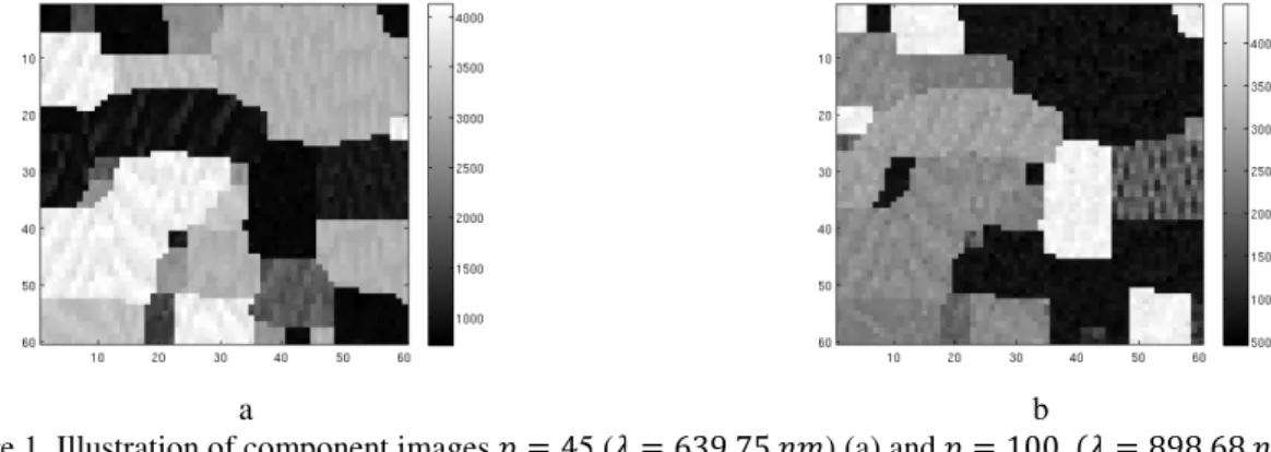
We have chosen to perform a comparative analysis of the four semi-blind methods, briefly recalled in the previous paragraphs, based on a small size (60x60 pixels) almost texture-free real hyperspectral image (100 spectral channels from 439.4 nm to 898.68 nm with spectral width from 4.47 nm to 4.76 nm).

Figures 1a and 1b present two different component images for illustration purpose. Figure 1a corresponds to the component image with channel index m = 45 and = 639.75 r, while Figure 1b shows component image with channel index m = 100 and = 898.68 r.

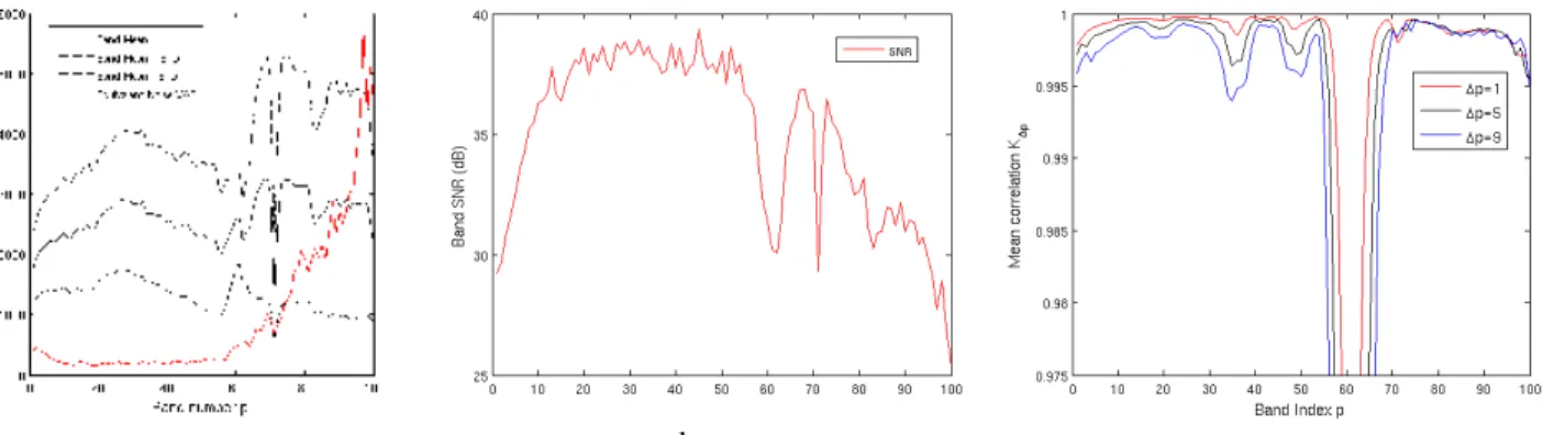
Figure 1. Illustration of component images m = 45 ( = 639.75 r) (a) and m = 100 = 898.68 r (b) The main statistics of the chosen hyperspectral image are shown along the spectral dimension in Figures 2a and 2b (only spectral channel indexes are specified on the horizontal axis from 1 to 100). Figure 2a shows mean value and rKO − MGs, rKO + MGs interval as well as the noise variance directly estimated from the data based on one of our method previously developed for estimating the equivalent noise variance in case of mixed noise [2].

As it can be seen in Figure 2b, tu is in the limits from about 25.33 sv till about 39.34 sv. The first half of component images are estimated as degraded with a low level of noise and the noise level increases quite considerably for the second half of the spectral channels. For the first part (m ∈ 1: 60 ), the estimated tu range is 29.22 sv, 39.34 sv

0 995 099 Ó 0.965 0 98 0 975 0 10 20 30 40 50 60 70 60 90 100 Band Index O p=1 O p=5 O p=9 35 30 25 I

5i

and the corresponding rD , rO interval for equivalent noise variance is 147.81,449.31 . For the second and complementary part (m ∈ 61: 100 ), both intervals become considerably larger and tu range is 25.33 sv, 36.85 sv while rD , rO interval for equivalent noise variance is 469.99,5834.98 .

a b c

To represent the correlation properties of the component images of the test image, we have calculated the mean correlation, denoted as w_∆y, between a current band m and its neighboring bands m − ∆_z and m + ∆_z (both distant from ∆z). Figure 2c displays the curves for ∆_z= 1, 5, 9 as a function of the band index m. Most of the neighboring component images are strongly correlated, with w , w_{ and w_| being very close to 1. The decrease in the neighborhood of the band 61 is due to the “red edge” transition in vegetation spectra.

To conclude the presentation of the chosen test image, the quite high variability in the dynamic range and the equivalent noise variance of its component images is conducive to an analysis of the experimental behavior of the four semi-blind image restoration methods under rather different realistic configurations (except the lack of textured content). We can also note that Figures 1a and 1b correspond to the least noisy (channel index m = 45, for which tu ~39 sv) and the most noisy (channel index m = 100, for which tu ~25 sv component images respectively.

Then, the component images of the chosen hyperspectral image have been locally spatially averaged, based on the classification results of the small data cube into 10 classes obtained beforehand [11] (contours between classes can be easily distinguished in Figures 2a and 2b). The component images thus spatially averaged have been subsequently blurred with various synthetic blurs (out-of-focus with diameter s = 7, Gaussian with ~ = 2, linear motion with length / = 7 and direction • = 135°) and degraded by signal independent noise with a SNR level corresponding to the SNR directly estimated previously from each component image. As done in [3], an adjustment including spatial alignment and intensity rescaling to the original image is systematically performed on both the degraded and the estimated component image before calculating the value of all criteria considered in the sequel.

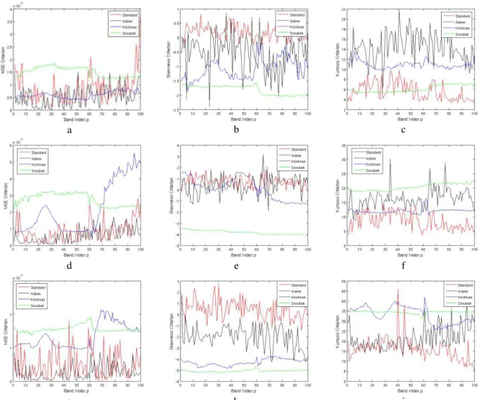
Now, the estimation accuracy of both the component image and the PSF by each of the four method in each spectral channel can be characterized by means of different qualitative and quantitative criteria. The first one among them is the estimation error bias distribution, as it exhibits clearly in distribution sense how a given method behaves globally over the spatial domain of a test component image (here 60x60 pixels). A further characterization of the estimation error bias distribution includes determination of the skewness and kurtosis measures. The skewness assesses the lack of symmetry of the distribution (skewness is zero for a normal distribution). Negative values for the skewness indicate that the bias is skewed left and positive values for the skewness indicate that the bias is skewed right. The kurtosis determines whether the bias is heavy-tailed (high value of kurtosis means occurrence of outliers) or light-tailed relatively to a normal distribution (for which the expected kurtosis value is 3).

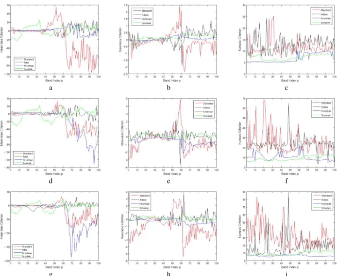
Fig. 3 presents the mean value on the image spatial domain (left column), skewness (middle column) and kurtosis (right column) properties of the image estimation error bias experimental distribution in each spectral channel for each of the four methods. First row (a) - (c) is for defocusing blur (s = 7), second row (d) - (e) for Gaussian blur (~ = 2) and third row (g) - (i) for linear motion blur (/ = 7, • = 135°). On average, we can deduct from the curves displayed in this figure Figure 2. Dynamic range (a) SNR (b) of a current band m and mean correlation w_∆y between a current band m and its neighboring bands distant from ∆_z (c)

S 11.73'so zo m 0 io PG 30 io o MI 10 BO 90 100 sand laexP o z0 00 +0 50 90 Bond Index p 00 90 100 SO 5-100 -000 2000 10 EO 30 I0 50 60 70 00 90 100 Band Ina %P 70 ä 40 10 0 10 PG d0 40 60 60 10 80 90 100 Bernd Index p o ro ao +o so so >o eo so 100 Band 40 20 -leu ZO 00 40 50 00 70 00 00 100 Hand Index p o io 20 30 4 02 70 eo so 100 Band Index 0 20 30 40 50 20 10 00 90 100 Band InE¢z p co 40 -20 v L0--60 - .,.han ro ao 40 50 so 70 00 so 100 Baneinevp

quite general tendencies, independently of the blur generated. All methods except the fourth one exhibit an almost centered image estimation error. All the methods share an experimental distribution close to a symmetrical one in the first part of spectral bands (m ∈ 1: 60 ), the least noisy ones. This holds except for the first method in case of a linear motion blur.

a b c

d e f

g h i

Figure 3. Mean value (left column), skewness (middle column) and kurtosis (right column) properties of the image estimation error bias experimental distribution in each spectral channel for each of the four methods. First row (a) - (c) is for defocusing blur (s = 7), second row (d) - (f) for Gaussian Blur (~ = 2) and third row (g) - (i) for Linear Motion Blur (/ = 7, • = 135°).

However, still in this part, the first two methods also show existence of outliers with a larger magnitude compared to those obtained with the other two methods (the kurtosis high value is confirmed by the error value at the frontiers between classes in the corresponding spatial bias map). In the second part of spectral channels (m ∈ 61: 100 ), the one corresponding to the noisier bands, the situation deteriorates to different extents for almost all methods. In this second part, the image mean estimation error remains weak and almost symmetrical for the second method and surprisingly for the fourth one (Sroubek) as well. Concerning outliers, the four methods rank in the same order as in the first part. One additional remark, worth noting is that there exists a quite wide variability in the behavior of methods over the whole spectral range, although the noise level is rather small (tu ≳ 25 sv) and does not vary too much.

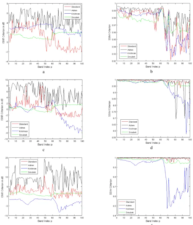
In addition to the estimation error bias, we have calculated other well-known quantitative blind assessment criteria, such as the increase of signal to noise ratio measure, denoted as ISNR (the difference between output and input SNRs, e.g. the input ones given in Figure 2b). Besides PSNR, we have also used the Structural Similarity Index Measure (SSIM) for measuring the similarity between restored and original images.The SSIM index values are in the range [0,1]

0.9 0.5 0.4 0 Standard Admm Krishnan Sroubek ' ' i 10 20 30 40 50 60 70 60 90 Band Index p 100 20 15 10 0 -10 Standard Admm Krishnan - Sroubek i 10 20 30 40 50 60 70 S0 90 Band Index p 100 0.65 -0.6 0.55 Standard Admm Krishnan - Sroubek 10 20 30 40 50 60 70 80 90 Band Index p 100 10 4 2 -2 -4 -10 Standard Admm Krishnan Sroubek i 10 20 30 40 50 60 70 30 90 100 Band Index p 0.99 0.96 E 0.97 ° Ú 0.96 2 cñ 0.95 0.94 0.93 0.92 0

4.

ivi,t

N

/\V

with higher values corresponding to closer proximity of both images [12]. It has the property of a unique maximum when the pixel values in the image neighborhoods are identical. The values of these two criteria are detailed in Figures 4 (a)-(f). As it is seen, for component images with less intensive noise (m ∈ 1: 60 ), efficiency of restoration is in general larger. Restoration efficiency decreases in the second part m ∈ 61: 100 ).

a b

c d

e f

Figure 4. ISNR (left column) and SSIM (right column) values obtained in each spectral band for each of the four methods. First row (a) and (b) is for defocusing blur (s = 7), second row (c) and (d) for Gaussian Blur (~ = 2) and third row (e) and (f) for Linear Motion Blur (/ = 7, • = 135°).

Both criteria are highly correlated and they rank the four methods in almost the same order. For this test dataset and according to default tuning of parameters involved in each of the four methods, the second method behaves more efficiently than first one. Both of them perform better than the other two methods. But they also prove a larger variability in results from one spectral band to another one, while neighboring spectral bands have been shown highly correlated in Figure 2c.

The last set of curves we describe now concentrates on the assessment of estimation accuracy of the other unknown of interest, namely the PSF. In general, we can expect that both the image and PSF estimations are closely linked together. Remind that at least one additional regularization term is specially introduced for each unknown in the cost function to reduce the search space for solutions and favor the research of a couple of solutions whose components have specific properties. Accordingly, it seems hardly possible to imagine the accurate estimation of one unknown with a poor estimation of the other unknown at the same time, in the case of a sufficient amount of regularization introduced for each unknown. However, it is also known in non-blind deconvolution that a small deviation of the PSF from the true one may lead to significant distortion in the image and vice versa.

Figures 5 (a)-(i) detail the value of the mean squared error, the skewness and kurtosis properties of the PSF estimation error bias distribution. We do not give here the value of the mean bias criterion as all four methods demonstrated a small value around zero of this criterion, independently of the three blurs considered. It can be seen from the analysis of the curves in these figures that the four methods rank again in the same order as the one obtained for the estimation of the image. Whatever the noise level, the first two methods are able to provide a lower mean squared estimation error, a more symmetrical experimental distribution of the estimation error compared to the other two methods (over the whole set of spectral bands from 1 to 100). The second method is even more accurate than the first one with respect to these two criteria. It is worth noting that the first method is the one providing the less amount of outliers in the PSF estimates for all three blurs considered. The other three methods give in general a higher amount of outliers, depending on the blur generated. For the defocusing blur (see Figure 5c), the fourth method behaves as efficiently as the first one, but the third and second methods generate an increasing number of outliers as compared to the other two methods. For the Gaussian blur (see Figure 5f), the third method, the second one and the fourth one show more outliers while classified in that order. And finally for the linear motion blur (see Figure 5i), there are two subsets of methods. The subset composed of the first and second methods provides less outliers than the subset of the third and fourth methods.

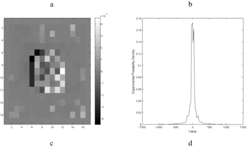
Let us finally perform visual analysis of one typical restoration result including both the estimation of the component image and the PSF through the analysis of the two corresponding spatial maps and empirical distributions of the associated estimation error bias in each case obtained on the noisiest component image m = 45, tu ~39 sv shown in Figure 2a blurred with the defocusing blur (s = 7) and noise level ~_‚= 14. As it can be seen, most of the errors are located on the contours between regions in the image and they are uniformly distributed over the PSF support (within the assumed upper limit of the PSF extent in the two spatial directions, set by default to 17x17 here).

Gathering all results obtained together, it appears that the second method is the one performing the best among the set of four methods comparatively assessed in this study. This result has been achieved on a specific test image for three different blurs with the same support size and different realistic noise level directly estimated from real data fragments. The first two methods show a global good restoration efficiency, but they are also characterized by a wide variability in results, even on neighboring bands which nevertheless share similar dynamic and noise properties. The last two methods seem less efficient, but behave in a more consistent and stable way.

-1500 -1000 -500 0 soo 1000 1500 Value 20 40 10 20 30 40 50 60 000 400 200 SO <5 ao 20 o 10 zo 00 IS só so 70 00 so 100 eana maex p o io zu zo ro so so 100 Band o 10 zo 30 +o 50 60 Band Index 00 90 100 ZO ° io en zo n ao ro an an ion cane eexp o Ca SO 10 50 60 10 CO SO 100 Band Index p II

4t11'4

Figure 5. Mean Squared Error (left column), skewness (middle column) and kurtosis (right column) properties of the PSF estimation error bias experimental distribution in each spectral channel for each of the four methods. First row (a) - (c) is for defocusing blur (s = 7), second row (d) - (f) for Gaussian blur (~ = 2) and third row (g) - (i) for linear motion blur (/ = 7, • = 135°).

010 0 14 0.0x -1500 -1000 -500 0 500 1000 1500 Value a b c d

CONCLUSIONS AND FUTURE WORK

We have presented the experimental results of a comparative analysis of a representative set of four semi-blind image restoration methods recently proposed. The regularization principles on which each of the four methods relies on have been shortly recalled beforehand. Then, experiments on a small size real texture-free hyperspectral image, the components of which have been spatially averaged and synthetically degraded with various synthetic blurs (out-of-focus, Gaussian, linear motion) and signal independent noise with a SNR level corresponding to the one directly estimated from the data have underlined peculiarities and practical behavior of each of the four methods on this specific dataset. According to the results obtained in this study, the second ADMM-based method is the one showing the best efficiency among the set of four methods comparatively assessed. Current and future works will extend our comparative analysis to a larger set of blurs (additional types and larger set of support sizes) and test images (including textures) before considering the blind multi-channel case, both for estimating the original image and the PSF.

Acknowledgements

The authors would like to thank all the authors of the blind methods comparatively assessed in this paper for making their code publicly available.

REFERENCES

[1] S. B. Hadj, Laure Blanc-Féraud, Gilles Aubert, “Space Variant Blind Image Restoration,” SIAM Journal on

Imaging Sciences, Society for Industrial and Applied Mathematics, 2014, 7, pp.2196 - 2225

[2] M. L. Uss, B. Vozel, V. V. Lukin and K. Chehdi, "Local Signal-Dependent Noise Variance Estimation From Hyperspectral Textural Images," IEEE Journal of Selected Topics in Signal Processing, vol. 5, no. 3, pp. 469-486, June 2011.

[3] M. S. C. Almeida and L. B. Almeida, “Blind and Semi-Blind Deblurring of Natural Images,” IEEE Trans. Image

Process., vol. 19, no. 1, pp. 36-52, Jan. 2010.

[4] M. S. C. Almeida and M. A. T. Figueiredo, “Blind image deblurring with unknown boundaries using the alternating direction method of multipliers,” IEEE Int. Conf. Image Process., ICIP 2013 - Proc., pp. 582-585, 2013.

[5] D. Krishnan, T. Tay, and R. Fergus, “Blind deconvolution using a normalized sparsity measure,” IEEE

Conference on Computer Vision and Pattern Recognition (CVPR), Providence, RI, pp. 233-240, 2011.

[6] F. Sroubek and P. Milanfar, “Robust Multichannel Blind Deconvolution via Fast Alternating Minimization,”

IEEE Trans. Image Process., vol. 21, no. 4, pp. 1687-1700, Apr. 2012.

Figure 6. Restoration results: spatial map of image estimation error bias (a) and its associated empirical distribution (b), spatial map of the PSF estimation error bias (c) and its associated empirical distribution (d) obtained for defocusing blur (s = 7) and noise level ~_‚= 14 on least noisy component image m = 45.

[7] M. S. C. Almeida and M. A. T. Figueiredo, “Parameter Estimation for Blind and Non-Blind Deblurring Using Residual Whiteness Measures,” IEEE Trans. Image Process., vol. 22, no. 7, pp. 2751-2763, Jul. 2013.

[8] T. F. Chan and C.-K. Wong, “Total variation blind deconvolution,” IEEE Trans. Image Process., vol. 7, no. 3, pp. 370-375, Mar. 1998.

[9] Y.-L. You and M. Kaveh, “Blind image restoration by anisotropic regularization,” IEEE Trans. Image Process., vol. 8, no. 3, pp. 396-407, Mar. 1999.

[10] Z. Xu, X. Chang, F. Xu and H. Zhang, "L1/2 Regularization: A Thresholding Representation Theory and a Fast Solver," in IEEE Transactions on Neural Networks and Learning Systems, vol. 23, no. 7, pp. 1013-1027, July 2012.

[11] B. Chen, K. Chehdi, E. De Oliveria, C. Cariou, B. Charbonnier, "Unsupervised component reduction of hyperspectral images and clustering without performance loss: application to marine algae identification", SPIE

ERS Conference: Image and Signal Processing for Remote Sensing, 26-29 September 2016, Edinburgh, United

Kingdom

[12] Z. Wang, A. C. Bovik, H. R. Sheikh, E. P. Simoncelli, Image quality assessment: from error visibility to structural similarity, IEEE Trans. on Image Processing, 8 (03), pp. 600-612, 2004.