Sampling and Meshing Surfaces with Guarantees

(1)

HAL Id: tel-00338378

https://pastel.archives-ouvertes.fr/tel-00338378

Submitted on 13 Nov 2008

HAL is a multi-disciplinary open access archive for the deposit and dissemination of sci-entific research documents, whether they are pub-lished or not. The documents may come from teaching and research institutions in France or abroad, or from public or private research centers.

L’archive ouverte pluridisciplinaire HAL, est destinée au dépôt et à la diffusion de documents scientifiques de niveau recherche, publiés ou non, émanant des établissements d’enseignement et de recherche français ou étrangers, des laboratoires publics ou privés.

Steve Y. Oudot

To cite this version:

Steve Y. Oudot. Sampling and Meshing Surfaces with Guarantees. Software Engineering [cs.SE]. Ecole Polytechnique X, 2005. English. �tel-00338378�

(2)

THESE

présentée et soutenue par Steve OUDOT

pour obtenir le titre de

DOCTEUR DE L’ÉCOLE POLYTECHNIQUE Discipline : Informatique

ÉCHANTILLONNAGE ET MAILLAGE DE SURFACES

AVEC GARANTIES

Thèse dirigée par Jean-Daniel Boissonnat

soutenue le 14 décembre 2005

Composition du jury :

M. Olivier Faugeras PRÉSIDENT M. Frédéric Chazal RAPPORTEUR

M. Gert Vegter RAPPORTEUR

M. Jean-Daniel Boissonnat DIRECTEUR M. Leonidas Guibas EXAMINATEUR

(3)

(4)

Remerciements

J’aimerais remercier en tout premier lieu Jean-Daniel Boissonnat, qui a dirigé ma thèse de manière à la fois fructueuse et conviviale tout au long de ces trois années. Le temps passé sous sa direction a été pour moi un véritable enrichissement intellectuel et personnel.

Je tiens également à remercier particulièrement Frédéric Chazal, dont les nombreuses remarques et suggestions ont contribué à améliorer significativement la qualité scientifique du mémoire, en particulier les chapitres 2 et 3. Les échanges que nous avons eus m’ont permis de mieux mettre en perspective mon travail, et d’établir des connexions avec d’autres branches des mathématiques.

Les chapitres 8 et 9 ne seraient sûrement pas ce qu’ils sont sans le concours de mes autres co-auteurs : Leo Guibas pour le probing, Mariette Yvinec et son étudiant Laurent Rineau pour le maillage de volumes à bords lisses. Qu’ils en soient remerciés.

Plus généralement, j’aimerais remercier les membres de l’équipe Géométrica pour les nombreuses discussions scientifiques et techniques que nous avons eues et pour la qualité constante de leurs remar-ques. Merci donc à Pierre Alliez, Frédéric Cazals, Raphaëlle Chaine, David Cohen-Steiner, Olivier Devillers, Sylvain Pion et Monique Teillaud.

J’aimerais aussi remercier personnellement les doctorants de l’équipe pour leur sérieux et leur en-train, ainsi que pour tous les bons moments passés ensemble. Camille, Christophe, Laurent, Marc, Marie, Thomas, un grand merci à vous tous. Enfin, last but not least, merci à Agnès pour son amitié et son aide précieuse.

Sur un plan plus personnel, je tiens à remercier Béatrice, ainsi que ma famille et mes proches, pour leur soutien et leur dévouement constants. En particulier, je leur sais infiniment gré d’avoir cru en mon travail aux moments où moi-même n’y croyais plus...

(5)

(6)

Introduction

In this thesis, we focus on one aspect of the problem of representing a continuous shape by a finite number of parameters. This issue finds applications in many areas of Science and engineering, where the goal is to perform computations and simulations on objects from the real world. Due to the finite amount of memory available on a computer, only discretized versions of these objects can be represented informatically.

It turns out that the choice of a specific representation depends highly on the application considered. Let us illustrate this claim with an example from the medical world. Recent technology allows to repre-sent the surface of any organ in a human body through a series of parallel slices, each slice containing the image of the contours of the organ in a certain plane. This kind of model is provided for instance by an MRI scanner. The problem with such a representation is that it is difficult to exploit, in contexts such as tumor or lesion tracking. Consequently, there is a real need for new kinds of representations. A whole area of research in image processing is devoted to this issue. Some solutions consist in con-verting the slice-to-slice model into a whole 3-dimensional image. Although this new representation is well-adapted to the tracking problem, it remains unsuitable for further processing. Moreover, the size of the data is a problem, since images are usually large, with a high definition.

Some representations are generically more effective than others. It is the case for simplicial meshes. Roughly speaking, a simplicial mesh is a collection of simplices of pairwise disjoint relative interiors, such that two simplices of the mesh either do not intersect, or intersect along a simplex of lower di-mension. We recall that a simplex of dimension d (or d-simplex, for short) is the affine hull of (d + 1) points. For instance, a 0-simplex is a point, a 1-simplex is a segment, a 2-simplex a triangle, a 3-simplex a tetrahedron, and so on. In this thesis, we focus mainly on simplicial meshes that approximate surfaces, a case in which all simplices have dimension at most 2. The mesh is then called a triangular mesh. Similarly, if all simplices have dimension at most 3, then the mesh is said to be a tetrahedral mesh.

Simplicial meshes are one of the most popular representations for surfaces, volumes, scalar fields and vector fields. Their success finds its origin in the fact that simplicial meshes are very well suited for many applications, such as visualization or numerical simulation. However, constructing a simplicial mesh that approximates a continuous object can be time-consuming, especially when the geometry of the object is complex. In this case, mesh generation becomes the pacing phase in the computational simulation cycle. Roughly speaking, the more the user is involved in the mesh generation process, the longer the latter is. An appealing example is given in [88], where the mesh generation time is shown to be 45 times that required to compute the solution. This motivates the search for fully-automated mesh-generation techniques.

(11)

This thesis addresses mainly the problem of constructing a triangular mesh to approximate a given surface. This problem is stated below in an informal manner. Some precisions will be given thereafter:

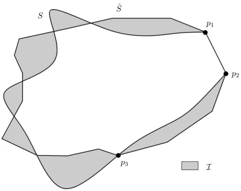
Surface mesh generation Given a surface S without boundary, construct a triangular mesh ˆS of

optimal size, that is both topologically equivalent to S and geometrically close to S.

The main concern here is that ˆSbe of same topological type as the input surface S. Since the surface S is assumed to have no boundary, this means that ˆSand S must have the same number of connected components and the same number of handles.

The surface mesh generation paradigm states also that ˆS must be geometrically close to the input surface S. This requires to define an accuracy measure. The Hausdorff distance is a good candidate and is therefore usually chosen. Recall that the Hausdorff distance between ˆSand S is ε if every point of ˆS is at distance at most ε from S, and every point of S is closer than ε to ˆS.

Concerning the size of the mesh, Agarwal and Suri [1] proved that, given a surface S, a threshold ε and a positive number k, it is NP-hard to decide whether there exists a mesh of size at most k that lies at Hausdorff distance at most ε from S. This means that it is hopeless to find effective methods to construct size-optimal meshes to approximate surfaces. Therefore, instead of constructing meshes of optimal size, our goal is rather to construct meshes that are as small as possible, typically of size within a constant factor of the optimal.

It is a well-known fact that, once the topology of ˆSis fixed, the numbers of faces of each dimension in the triangular mesh are fully determined by the number of its vertices. Therefore, bounding the size of ˆScomes down to bounding the number of its vertices. The mesh generation process reduces then to two steps:

S1 Construct a finite set of points E sampled from the surface S.

S2 Connect the points of E with triangles, so that the underlying triangulation ˆS has the same topo-logical type as S.

The quality of a surface meshing algorithm is clearly measured by the quality of its output. The better the approximation, the better the algorithm. But another criterion has to be taken into account: the amount of information on the input surface S needed by the algorithm. Meshing strategies that use few geometric predicates will be easier to implement, and their algorithmic complexity will be less dependent on the topological and geometric complexity of the surface S. Moreover, the nature of the information available on S varies with the context. Geometric queries are more or less difficult, depending on the way the surface S is defined. For instance, computing the principal curvatures of S at a given point is easy when S is defined as a level-set of some function f whose closed formula is known. However, this task becomes very difficult when no closed formula of f is known, as it is the case for instance when S is defined as a level of grey in a 3-dimensional image or as the result of a PDE. In this respect, algorithms that use fewer predicates are not only easier to implement, but they turn out to be also more generic since their predicates can be implemented in a wider range of applications.

We distinguish between three variants of the surface meshing problem, depending on the way the surface S is defined and on the amount (and nature) of information available as input. In fact, there are

(12)

many more variants, but to our knowledge, each of them can be reduced to one of the following: surface reconstruction, surface sampling, and surface probing.

I.1 Surface reconstruction: working out sampling conditions

In surface reconstruction, the surface S is known only through a finite set of points E sampled from S. This point set can come from various sources, such as for instance from range scanning data. The point sample E is given as input, and the goal is simply to build a connectivity between the points of E, so that the resulting mesh ˆS approximates S topologically and geometrically. This reduces the problem to the step S2 described above.

Several provably good methods have been proposed to solve the smooth surface reconstruction prob-lem. We refer the reader to [30, 31] for a comprehensive survey. The proofs of correctness of these methods rely on sampling conditions that control the local density of the input point set E.

Closed Ball Property The first sampling condition was introduced by Edelsbrunner and Shah [63] and is called the Closed Ball Property. It states that every d-face of the Voronoi diagram of E has an intersection with S that is either empty or topologically equivalent to a d-ball. Edelsbrunner and Shah proved that, under this condition, some subcomplex of the Delaunay triangulation of E, called Del_|S(E), has the same topological type as S. Del_|S(E)will be described more in detail in the next chapter. Unfortunately, the Closed Ball Property guarantees only the topology of the reconstruction, not its geometry.

µ-samples Amenta and Bern [6] proposed then the µ-sampling condition. Roughly speaking, a finite subset E of a surface S is a µ-sample of S if every point p of S is closer to E than µ dM(p), where dM : R3 → R denotes the distance to the so-called medial axis M of S, defined in Chapter 1. This condition requires that the surface S be smooth.

Amenta and Bern proved that, if E is a µ-sample of S, for a sufficiently small µ, then the Closed Ball Property of Edelbrunner and Shah is satisfied. Hence, Del_|S(E)has the same topological type as S. They also proved that Del_|S(E)lies at Hausdorff distance c(S) µ2from S, where the constant c(S) depends only on S. In addition, Del_|S(E)provides good approximations of the normals of S [6], of its area [92], and of its curvatures [49]. Therefore, if the input point set E is a µ-sample of S, then the problem of reconstructing S from E comes down to finding which faces of the Delaunay triangulation of E belong to Del_|S(E). A number of provably good reconstruction algorithms are based on this approach [6, 7, 8, 19, 53, 54, 55].

Several variants of the concept of µ-sample appeared since [6], in particular the so-called uniform ε-samples [10], whose density is specified by a uniform sizing field equal to a constant ε. In order to use a single concept, we introduce the following

Definition I.1 Given a surface S and a positive function σ : S → R, a finite point set E ⊂ S is a σ-sample of S if ∀p ∈ S, E ∩ B(p, σ(p)) 6= ∅.

(13)

From now on, a µ-sample in the sense of [6] will be called a µdM-sample, whereas a uniform ε-sample in the sense of [10] will be referred to as an ε-ε-sample, according to Definition I.1. Note that both concepts are closely related. Indeed, any ε-sample of S is a µdM-sample for some µ depending on ε, and reciprocally, any µdM-sample of S is an ε-sample for some ε depending on µ. Therefore, the theoretical guarantees offered by µdM-samples hold for ε-samples as well, provided that ε is small enough. Specifically, ε must be less than a fraction of the reach of S, which is the infimum of dMover S. This infimum is positive when dMis positive. The surface S is then said to have a positive reach.

The noisy case The ε-sampling condition, as defined above, assumes that the points of E belong to S. In practice, due to the fact that scanners can only measure points within a given precision, the points of Eusually do not lie exactly on the surface S.

Dey and Goswami [56] proposed an extension of the cocone algorithm [55] that solves this variant of the reconstruction problem, provided that the input point set E is a so-called noisy µdM-sample of

S, which is equivalent to an ε-sample, with the difference that the points may not lie on S but must be closer to S than a fraction of their distance to the medial axis of S.

The nonsmooth case The µ-sampling condition assumes also that the surface is smooth. The distance to the medial axis of a nonsmooth surface S vanishes at the points where S is not differentiable. As a consequence, the reach of S is zero, and no finite subset of S is a µdM-sample of S. This makes µ-samples useless in this context. Nevertheless, ε-samples are still well-defined if ε is positive, but the theoretical guarantees of [6] no longer apply since ε > 0 is not smaller than a fraction of the reach of S. Chazal and Lieutier [35] introduced the so-called weak feature size, or wfs for short. Let dS : R3 → R+map each point of R3to its distance to S. The weak feature size is simply the smallest critical value of dS, in the sense of Riemannian geometry [69, 74].

The advantage of the weak feature size, over the distance to the medial axis, is that the class of objects with positive wfs is much larger than the class of objects with positive reach. This allows to construct ε-samples, with ε ≤ wfs, on a wide variety of smooth and nonsmooth shapes.

Chazal and Lieutier did not exhibit any subcomplex of Del_|S(E)with the same topological type as S. However, they showed that the homology groups of the 3-dimensional object O bounded by S can be retrieved from any noisy wfs-sample1 _E _{of S. The approach consists in applying persistence} techniques [62] on a specific filtration of Del(E), to compute the homology groups of O. Furthermore, an approximation of the medial axis of the object O can be computed from the Voronoi diagram of E.

The approach of Chazal and Lieutier is very generic and works in the nonsmooth and noisy setting. However, it provides information exclusively on the topology of the object, not on its geometry.

Other approaches To complete our overview of previous work on surface reconstruction, let us em-phasize that many other methods have been proposed to solve the reconstruction problem. Some of them interpolate the point set E, others define surfaces that approximate E. However, almost all these meth-ods come with no theoretical guarantees regarding the topology of the approximation. Two noticeable exceptions are the approach of [79], based on Moving Least Squares techniques [83], and the method

1_{In the same sense as Dey and Goswami, except that d}

(14)

of [19], based on natural neighbor coordinates [18]. Both methods can guarantee the topology of their approximating surface, under ε-sampling conditions.

I.2 Surface sampling: satisfying the sampling conditions

Here, the surface S is given in a form that allows to sample new points from S. For instance, S can be defined implicitely, as a level set of some real-valued function defined over R3.

This issue is somehow dual to the surface reconstruction problem. Indeed, in surface reconstruction, the point set E is given as input, and the goal is to find sampling conditions that guarantee a correct reconstruction. In surface sampling, the goal is to build a point set E that satisfies some sampling condition, so that correct reconstruction is then ensured. In other words, surface sampling focusses on step S1 of the mesh generation process, whereas surface reconstruction focusses on step S2.

The main drawback of the ε-sampling condition is that, given a surface S and a positive value ε, it is difficult to check whether a sample is an ε-sample of S, and even more difficult to construct an ε-sample of S. This is due to the fact that a direct application of the definition of an ε-sample leads to complicated operations like cutting the surface S with balls. This is why previous work on surface sampling does not rely on this condition.

It is only recently that provably good sampling and meshing techniques appeared in the literature. Some of these techniques handle only restricted types of shapes, such as piecewise parametric CAD models [104, 112], Van der Waals and solvent-excluded molecular surfaces [81], or skin surfaces [38, 39, 80]. We do not consider them in the sequel.

The other provably good algorithms can only handle smooth surfaces. Moreover, to our knowledge, all these algorithms require that the surface S be defined implicitely, as a level-set of some function f of known closed formula. Although it is well-known that every surface S without boundary is the zero-set of some real-valued function defined over R3 _{(take for instance the signed distance to S), the} assumption that a closed formula of f is known is very restrictive in practice, since in many applications (for instance sampling an isosurface in a 3-dimensional image) no closed formula of f is known a priori. We classify the existing algorithms with respect to the amount of information on S they require:

1. The implicit surface mesher of Plantinga and Vegter [96] generates an adaptive grid and then ap-plies the Marching Cubes algorithm [87]. Using interval arithmetics, Plantinga and Vegter can certify the topology of ˆS. Moreover, by refining the grid sufficiently, they can achieve any given bound on the Hausdorff distance between ˆSand S. This is a significant step since the Marching Cubes algorithm and its variants [44] usually come without any topological or geometric guaran-tees. However, the use of interval arithmetics requires to now the gradient of f.

2. Algorithms based on the Closed Ball Property of Edelsbrunner and Shah [63], like the implicit surface mesher of Cheng et al. [42], require to be able to compute the critical points of height functions on the restrictions of S to some hyperplanes. The topology of the output mesh is ensured thanks to the Closed Ball Property.

3. Methods based on critical points theory [20, 76] require to compute the critical points of f, as well as their indices, which is an even more involved computation, although it can be performed using interval arithmetics.

(15)

The above techniques work only in the smooth setting. Recently, Dey et al. adapted the method of [42] to the case where S is a polyhedron that approximates a smooth surface [57]. This assumption on S allows the authors to use the same mathematical tools as in the smooth setting, but it is quite restrictive for practical applications. To our knowledge, no provably good sampling algorithm has ever been proposed for the nonsmooth non-polyhedral case.

I.3 Surface probing: reducing the required knowledge of the surface

Surface probing, also known as blind surface approximation or interactive surface reconstruction, con-sists of discovering the shape of an unknown object O through an adaptive process of probing its surface S from the exterior. A probe is issued along a ray whose origin lies outside O and returns the first point of O hit by the ray. Successive probes may require the probing device to be moved through the free space outside O. The goal is to find a strategy for the sequence of probes that guarantees a precise approximation of S after a minimal number of probes.

This problem belongs to the class of geometric probing problems, pioneered by Cole and Yap [50]. Geometric probing is motivated mainly by applications in robotics. In this context, our probe model described above is called a tactile or finger probe. Geometric probing also finds applications in other areas and gave rise to several variants. In particular, other probe models have been studied in the liter-ature, e.g. line probes (a line moving perpendicular to a direction), X-ray probes (measuring the length of intersection between a line and the object), as well as their counterparts in higher dimensions.

The existing probing algorithms can be classified into two main categories, exact or approximate, depending on whether they return the exact shape of the probed object or an approximation. An exact probing algorithm can only be applied to shapes that can be described by a finite number of parameters like polygons and polyhedra. Therefore, exact probing is too restrictive for most practical applications. Approximate probing algorithms overcome this deficiency by considering the accuracy of the desired reconstruction as a parameter. The goal is to find a strategy that can discover a guaranteed approximation of the object using a minimal number of probes. This issue is closely related to surface sampling. However, it differs in an essential way: here, the surface S is known through an oracle, the probing device, which can answer only very specific geometric questions.

Most of the work on exact geometric probing is for convex polygons and polyhedra – see [106] for a survey of the computational literature on the subject. Nevertheless, it has been shown that, using enhanced finger probes, a large class of non convex polyhedra can be exactly determined [2, 24]. Con-cerning approximate probing, an important class is the class of convex shapes. Probing strategies have been proposed for planar convex objects using line probes [86, 97] and some other probe models are analyzed in [98]. However, as far as we know, designing provably good techniques to probe non convex non polyhedral objects has not been considered prior to this thesis.

I.4 Overview of the thesis and contributions

In this thesis, the surface S can be smooth or nonsmooth, but the devices used for taking measures on S provide exact information. As a consequence, the points of E belong to S.

(16)

Sampling conditions In Part A, we introduce the concept of loose ε-sample, which can be viewed as a weak version of the notion of ε-sample. The main advantage of loose ε-samples over ε-samples is that they are easier to check and to construct. Indeed, checking that a sample is a loose ε-sample reduces to checking whether a finite number of spheres have radii at most ε.

When the surface S has a positive reach, we prove that, for sufficiently small ε, ε-samples are loose ε-samples, and reciprocally. As a consequence, loose ε-samples offer the same topological and geometric guarantees as ε-samples.

We also focus on the case where S is nonsmooth. In order to make geometric claims, we restrict our study to a subclass of the objects with positive weak feature size: the so-called k-Lipschitz surfaces, defined in Chapter 2. This subclass contains all objects with positive reach, but also all sufficiently

smooth polyhedra (see Definition 2.7), as well as a number of other nonsmooth shapes with non-trivial

topology. We prove that, if S is a k-Lipschitz surface and E is a (loose) ε-sample of S, for sufficiently small k and ε, then Del_|S(E)has the same topological type as S and is close to S for the Hausdorff distance. Our theoretical results hold provided that the inner angles of the facets of the Delaunay trian-gulation of E are not too small, which is ensured by assuming that the points of E are farther than a fraction of ε from one another. This sparseness condition is known to be a bit restrictive in the context of surface reconstruction. However, it can be easily satisfied in the contexts of surface sampling and surface probing.

A simple surface sampling algorithm In Part B, we show how our sampling condition can be turned into a simple and efficient surface mesh generator. The latter is based on a Delaunay refinement tech-nique, which consists in constructing an initial mesh and then refining iteratively the elements of the mesh that do not meet some user-defined size or shape criteria. This greedy tehnique was pioneered by Ruppert [99] in the plane, and then extended by Chew to surfaces in 3-space [45]. Our mesher derives from Chew’s algorithm. It takes as input a user-defined parameter ε and an initial point set EI ⊂ S, and it outputs a loose ε-sample EF of S, together with Del_|S(EF).

Chew did not provide his algorithm with any topological guarantees. Here, taking advantage of the theoretical results of Part A, we can prove that the output mesh is a manifold without boundary, with the same topological type as S and close to S for the Hausdorff distance, provided that ε is chosen sufficiently small. Specifically, ε must be less than a fraction of the reach of S when the latter is smooth, and less than a fraction of the so-called Lipschitz radius of S (defined in Chapter 2) when S is k-Lipschitz, for sufficiently small k. It follows that the algorithm generates provably good meshes on a wide class of smooth and nonsmooth shapes. Moreover, we show that the number of points sampled from S by the algorithm lies within a constant factor of the optimal.

Let us emphasize that our mesh generator maintains the 3-dimensional Delaunay triangulation of the point sample throughout the process. This is mandatory for guaranteeing the topology of the output mesh. Maintaining a whole 3-dimensional triangulation can be time-consuming in general. However, we prove in our case that the size of the data structure remains bounded, which implies that the space and time complexities of the algorithm are quite reasonable. Further detail is provided in Chapter 4.

(17)

A unified solution to the meshing problem A noticeable feature of the algorithm is that it needs only to know the surface S through an oracle that can compute the intersection of any given segment with S. Therefore, our mesh generator is generic enough to be applied in a wide variety of contexts. This genericity is illustrated in Part C, where we show that the algorithm can be used to mesh implicit surfaces, remesh polyhedra, or reconstruct surfaces from scattered data points. Our approach to surface reconstruction is similar to that of [19]. It consists of defining an implicit function f0 _{from the input} point set, and then to mesh the zero-set S0 _{of f}0 _{using our mesh generator. Combining our theoretical} results with those of [19], we can certify the topology and geometry of the output mesh. Note that no closed formula of f0 _{is available, hence none of the implicit surface sampling techniques presented in} Section I.2 can be applied in this context.

We also show that the algorithm can be easily adapted to probe unknown objects. The approach consists of using the probing device as an oracle for our mesh generator. This oracle is weaker than the one used above, since it can detect only the first intersection point of a given segment with the surface S. Moreover, before checking the intersection of a given segment s with S, the probing device must first be moved to an endpoint of s. Therefore, we cannot check the intersections of all the segments with S. We prove however that this version of the algorithm comes with the same theoretical guarantees as the original version, regarding the quality and the size of the output.

Finally, we show that our meshing technique can be extended to construct tetrahedral meshes ap-proximating 3-dimensional objects with curved boundaries, such that the mesh elements (tetrahedra and triangles) conform to some user-defined size and shape criteria. The idea is to exploit the fact that the algorithm maintains a whole 3-dimensional Delaunay triangulation. Whenever a tetrahedron does not meet the size or shape requirements, it is refined by inserting its circumcenter. The output point set is no longer a subset of S. Moreover, the output mesh contains all Delaunay tetrahedra whose circumcenters lie in the object O to mesh. Using our theoretical results on the approximation of the boundary of O, we can certify the output of the algorithm.

Our contributions at a glance We list our main contributions below:

• A new sampling condition, called loose ε-sampling, which offers the same topological and geo-metric guarantees as the classical ε-sampling condition in the smooth setting, but which is much easier to check and to construct.

• A theoretical analysis in the nonsmooth Lipschitz setting, which proves that (loose) ε-samples offer the same guarantees in this context as in the smooth setting, provided that an additional sparseness condition is satisfied. As a consequence, ε-sampling and loose ε-sampling are the first sampling conditions to provide both topological and geometric guarantees in the nonsmooth setting.

• A simple meshing algorithm that can provably well approximate smooth or Lipschitz surfaces, with a number of points that lies within a constant factor of the optimal. This algorithm is one of the few certified methods for the smooth and the polyhedral cases, and the first certified method for the nonsmooth non-polyhedral case. We have implemented it in a number of practical

(18)

sit-uations: isosurface extraction from 3D medical images, polygonal surface remeshing, etc. Our experimental results provide evidence that the approach is very effective in practice.

• An easy (yet certified) adaptation of our algorithm that solves the surface probing problem in the case of a convex or non-convex object with curved boundaries. No certified solution was known for this problem prior to this work.

• A natural extension of our algorithm that constructs provably good tetrahedral meshes to approxi-mate 3-dimensional objects with curved boundaries. It is the first certified solution ever proposed for this problem. Moreover, our preliminary experimental results are quite promising, regarding the practicality of the approach.

(19)

(20)

Preliminaries

This chapter introduces most of the mathematical concepts that will be used in the thesis.

Basic notations

Throughout the thesis, R3 _{is the ambient affine space. Points are written in italic font, e.g. p, q, and} vectors in bold font, e.g. n, n0.

R3is endowed with a canonical frame (o, ex,ey,ez). For any point p, we call p the vector that goes from the origin o of the frame to p. The usual inner product of two vectors n, n0 _{is denoted n · n}0_{, and} defined by

n · n0 ₌_n

xn0x+nyn0y+nzn0z,

where nx,ny,nz and n0x,n0y,n0z are the coordinates of n and n0 in the canonical basis (ex,ey,ez). We abuse notations and write n2 the inner product of n with itself. In addition, we denote n × n0 the outer product of n, n0_{, defined by} n × n0₌ ¯ ¯ ¯ ¯ ¯ ny n0y nz n0z ¯ ¯ ¯ ¯ ¯ ex+ ¯ ¯ ¯ ¯ ¯ nz n0z nx n0x ¯ ¯ ¯ ¯ ¯ ey+ ¯ ¯ ¯ ¯ ¯ nx n0x ny n0y ¯ ¯ ¯ ¯ ¯ ez

Finally, we denote by (n, n0₎_{the modulus of the angle (measured in [−π, π]) between vectors u and v.}

Distances and topology

We call k.k the Euclidean norm:

∀n ∈ R3, _{knk =}√n2 ₌√n · n

For any points p, q, d(p, q) denotes the Euclidean distance from p to q, defined by d(p, q) =kp − qk

Given a point c and a positive constant r, B(c, r) denotes the ball of center c and radius r. Unless otherwise specified, the ball B(c, r) is closed.

The affine space R3 _{is canonically endowed with the topology generated by the set of open balls.} Given a subset X of R3_{, int(X), ¯}_{X, and ∂X denote respectively the interior, the closure, and the} boundary of X. Moreover, we call diam(X) the Euclidean diameter of X:

diam(X) = sup_{{d(p, q), p ∈ X, q ∈ X}} xi

(21)

We now introduce two topological concepts that will be widely used in the thesis. We refer the reader to [14] for further detail.

Definition P.2 Two topological spaces X, Y are homeomorphic if there exists a continuous and

bijec-tive map h : X → Y such that h−1 _{is continuous. The map h is called a homeomorphism from X}

to Y .

If X, Y are subsets of R3_{, and if h is a homeomorphism from R}3_{to R}3_{, such that h(X) = Y , then} his said to be an ambient homeomorphism from X to Y .

Definition P.3 Two topological spaces X, Y embedded in R3 _{are isotopic if there exists a continuous}

map i : [0, 1] × X → R3 such that i(0, .) is the identity over X, i(1, X) = Y , and for any t ∈ [0, 1], i(t, .)is a homeomorphism from X onto its image. The map i is called an isotopy from X to Y .

If i is an isotopy from R3 to R3 such that i(1, X) = Y , then i is said to be an ambient isotopy from Xto Y .

We need also to define distances between subsets of R3. Given a point p and a subset X of R3, the distance from p to X is denoted d(p, X) and defined as follows:

d(p, X) = inf{d(p, q), q ∈ X}

If X = ∅, then d(p, X) is infinite. Otherwise, d(p, X) is finite and non-negative. Moreover, d(p, X) = 0 iff (if and only if) p belongs to the closure ¯Xof X.

Definition P.4 Given two subsets X and Y of R3_{, the Hausdorff distance between X and Y is} d_H(X, Y ) = max_{sup

p∈X

d(p, Y ), sup q∈Y

d(q, X)_}

Note that dH(X, Y ) = 0iff ¯X = ¯Y.

Definition P.5 Given two homeomorphic subsets X and Y of R3_{, the Fréchet distance between X and} Y is

d_F(X, Y ) = inf

h _p∈Xsup d(p, h(p))

where h ranges over all homeomorphisms from X to Y .

Observe that, for any homeomorphism h : X → Y and any point p ∈ X, we have d(p, h(p))≥ max{d(p, Y ), d(h(p), X)},

thus d_F(X, Y )≥ dH(X, Y ). It follows that any upper bound on the Fréchet distance of X, Y is also an upper bound on their Hausdorff distance.

(22)

Geometric measures

We will use two geometric measures: the Lebesgue measure L2_{on R}2_{, and the 2-dimensional Hausdorff} measure H2_{on R}2_{and R}3_{. We borrow their definitions from [91].}

Definition P.6 There is a unique Borel-regular, translation-invariant measure on R2_{, such that the}

mea-sure of the unit cube [0, 1]2_{is 1. This measure is called the Lebesgue measure and noted L}2_.

Note that L2_{is defined only on R}2_{. Hence, it tells nothing about the area of a surface of R}3_{, a notion} that will be extensively used in this thesis, especially in Chapter 3.

Definition P.7 Given X ⊂ Rn _{(n ≥ 2), the 2-dimensional Hausdorff measure of X, or H}2_(X)_for

short, is defined as follows:

H2(X) = lim δ→0+ inf X ⊂S iXi diam(Xi) ≤ δ +∞ X i=0 π µ diam(Xi) 2 ¶2 (1)

The infimum in (1) is taken over all countable coverings {Xi} of X whose members have Euclidean diameter at most δ. It is proved in [91, §2.3] that the limit always exists, and that H2is a Borel-regular measure over Rn_{, for any n ≥ 2. A more comprehensive proof can be found in [67, §2.10].}

The 2-dimensional Hausdorff measure coincides with L2_{on R}2_{. Moreover, it generalizes the notion} of area of a surface. Specifically, H2_(S)coincides with the usual area of S, for any C1-continuous 2-dimensional submanifold of Rn_{, n ≥ 2.}

Surfaces

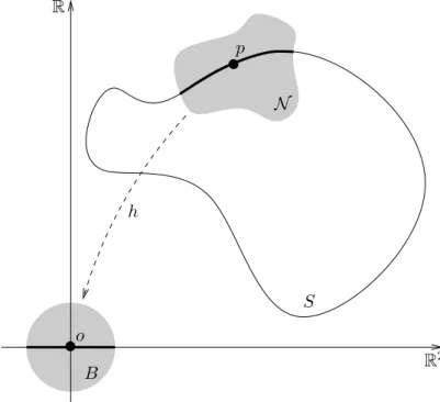
Throughout the thesis, S is a C0_{-continuous 2-dimensional submanifold of R}3_{. Informally, this means} that, for any point p ∈ S, there exists an open neighborhood N of p in R3that can be mapped to the unit open ball B by some homeomorphism h, such that h(p) is the origin o and h(N ∩ S) = B ∩ R2_{. See} Figure 1 for an illustration. We refer the reader to [14, §2.1.1] for a formal definition.

For simplicity, we say that S is a surface without boundary. We call M its medial axis, defined in Section 1.1.1. If S is differentiable at p, then T (p) and n(p) denote respectively the tangent plane and the unit normal vector (pointing outwards) of S at p.

Complexity

Given two positive functions f, g defined over R+, we use the notation f = O(g) to indicate that there exists a non-negative constant ν such that ∀x ≥ 0, f(x) ≤ ν g(x). Moreover, f = Ω(g) stands for g = O(f ), and f = Θ(g) means that we have both f = O(g) and f = Ω(g).

Unless explicitely mentioned, the constant ν in the above statements is absolute. Some of our results use these notations in a context where the constant ν depends on the surface S. In such a case, we write f = OS(g), f = ΩS(g), f = ΘS(g), instead of f = O(g), f = Ω(g), f = Θ(g).

(23)

PSfrag replacements o S p N R2 R B h

Figure 1: A surface without boundary.

(24)

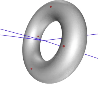
Figure 3: A case where Del_|S(E)is empty: the four points of E are placed on a torus, such that the Voronoi edges pass through the hole.

Voronoi diagrams and Delaunay triangulations

We now present several objects of the Computational Geometry that will be used throughout the thesis. Let E be a finite set of points of R3_.

• The Voronoi cell of p ∈ E is the set of all points of R3that are closer to p than to any other point of E. The Voronoi diagram of E, Vor(E), is the cellular complex formed by the Voronoi cells of the points of E.

• The dual complex of Vor(E) is a tetrahedrization of the convex hull of E, called the Delaunay

triangulation of E and noted Del(E). For any face f (vertex, edge, facet or cell) of Del(E), V(f)

denotes the face of Vor(E) dual to f.

• By VG(E) we denote the 1-skeleton graph of Vor(E), also called Voronoi graph of E.

The mesh generator introduced in Part B of this thesis relies on a subcomplex of Del(E), defined below: • We call Delaunay triangulation of E restricted to S, and we note Del|S(E), the subcomplex of Del(E)that consists of the facets of Del(E) whose dual Voronoi edges intersect S. An example is given in Figure 2. An edge or vertex of Del(E) belongs to Del_|S(E)if it is incident to at least one facet of Del_|S(E). Notice that we depart from the usual definition [45, 63] and do not consider vertices and edges with no incident facet of Del_|S(E). See Figure 3 for an illustration.

• A facet (resp. edge, vertex) of Del|S(E)is called a restricted Delaunay facet (resp. restricted

Delaunay edge, restricted Delaunay vertex). For a restricted Delaunay facet f, we call surface Delaunay ball of f any ball circumscribing f centered at some point of S ∩ V(f). Notice that the

(25)

• Given a vertex v of Del|S(E), we call star of v the union of all the facets of Del|S(E)incident to v.

• Given a facet f of Del|S(E), we call neighborhood of f, of N(f) for short, the union of all the facets of Del_|S(E)that are non-disjoint with f (including f itself).

In the sequel, u, v, w denote vertices of Del_|S(E), whereas p, q denote points of R3.

Quality measures for mesh elements

In this thesis, our aim is to generate triangular and tetrahedral meshes with well-sized and well-shaped elements:

• Given a positive sizing field σ, a simplex of circumcenter c is said to be well-sized if its circum-radius is at most σ(c).

• Following [103], we say that a simplex is well-shaped if its aspect ratio is less than a given thresh-old. The aspect ratio of a simplex is the ratio between its circumradius and the radius of its inscribed sphere.

Another shape quality measure will be used in the thesis: the so-called edge ratio. The radius-edge ratio of a simplex is the ratio between its circumradius and the length of its shortest radius-edge. Any triangle with a small radius-edge ratio has a small aspect ratio. This property does not hold however for tetrahedra: the so-called slivers have small radius-edge ratios but a large aspect ratios. Roughly speaking, a sliver is a tetrahedron whose vertices are close to a great circle of its circumsphere and equally spaced along this circle. See [41] for additional information on this topic.

(26)

Sampling Conditions

(27)

(28)

Introduction

In this part of the thesis, we introduce the concept of loose σ-sample and we study its various prop-erties on smooth and on Lipschitz surfaces. Our theoretical results will be instrumental in proving the correctness of our sampling algorithm, in Part B.

The concept of loose σ-sample can be viewed as a weak version of the notion of σ-sample. The main advantage of loose σ-samples over σ-samples is that they are easier to check and to construct. Indeed, checking that a sample is a loose σ-sample reduces to checking whether a finite number of spheres are small enough with respect to the value of the sizing field σ at their centers.

Definition A.1 Given a surface S and a positive function σ : S → R, a finite point set E ⊂ S is a loose σ-sample of S if the following conditions are satisfied:

1. ∀p ∈ S ∩ VG(E), E ∩ B(p, σ(p)) 6= ∅,

2. Del_|S(E)has vertices on all the connected components of S.

Since the centers of the surface Delaunay balls are precisely the intersection points of S with the Voronoi edges, Condition 1 of Definition A.1 is verified iff every surface Delaunay ball B(c, r) has a radius r ≤ σ(c).

Observe that Condition 1 alone is not sufficient to control the density of E. Indeed, according to our definition of the restricted Delaunay triangulation, a point of E is a vertex of Del_|S(E)only if at least one edge of the boundary of its Voronoi cell intersects S. It follows that some of the points of E may not be vertices of Del_|S(E). In some situations (see Figure 3 for an example), Del_|S(E)may even be empty, in which case Condition 1 is trivially verified for any positive function σ, but not Condition 2.

Note to the reader: In the sequel, σ is assumed to be bounded from above by some constant ε. As a

consequence, any (loose) σ-sample is a (loose) ε-sample. This assumption allows us to use a single concept throughout the thesis, namely the concept of (loose) ε-sample. Moreover, it simplifies the proofs in the smooth setting.

In Chapter 1, we focus on the case where the surface S is smooth. In this context, we show that loose ε-samples of S enjoy the same topological and geometric properties as ε-samples of S, provided that εis small enough. These properties trivially hold for (loose) σ-samples as well, provided that σ ≤ ε. In addition, we prove that loose ε-samples and ε-samples are equivalent asymptotically, when ε goes to zero.

Chapter 2 deals with the more general case where S is a k-Lipschitz surface, smooth or nonsmooth. We show that, for sufficiently small k and ε, (loose) ε-samples offer the same guarantees in this context as in the smooth setting, provided that an additional sparseness condition is satisfied – see Section 2.2. These properties trivially hold for (loose) σ-samples as well, provided that σ is at most ε and satisfies the sparseness condition of Section 2.2. In addition, like in the smooth setting, we prove that loose ε-samples and ε-samples are equivalent asymptotically, when ε goes to zero.

In Chapter 3, we work out a lower bound on the size of (loose) ε-samples. This bound holds both in the smooth and in the Lipschitz settings. Moreover, we show that, under a mild sparseness condition2 introduced in Definition 3.2, the size of any (loose) ε-sample is also bounded from above.

(29)

(30)

The Smooth Case

In this chaper, we focus on the case where the surface S is smooth. By smooth, we mean that S is C1,1-continuous, i.e. it is continuously differentiable and its normal satisfies a Lipschitz condition. We assume without loss of generality that the normal of S is oriented consistently, say it always points outwards.

In Section 1.1, we recall a few known facts about smooth surfaces and their medial axis, defined below. We also prove several local properties of loose ε-samples. In Section 1.2, we review the main global properties of loose ε-samples. Specifically, we prove that their restricted Delaunay triangulation is a manifold without boundary (1.2.1), isotopic to S (1.2.2) and at Fréchet distance OS(ε2₎ from S (1.2.3). In Section 1.3, we show that loose ε-samples and ε-samples are closely related. To complete our study, we give additional properties in Section 1.4, that will not be used in this thesis but which can be useful in some applications. Finally, in Section 1.5, we recall analogous results that were proved in [23] for (loose) µdM-samples.

1.1 Preliminaries

1.1.1 Positive reach

The medial axis of S, noted M, is the topological closure of the set of points of R3that have more than one nearest neighbor on S. For a point p ∈ R3_{, we call distance to the medial axis at p, and write} dM(p), the Euclidean distance from p to the medial axis of S. As noticed by Amenta and Bern [6], dM is 1-Lipschitz, i.e.

∀p, q ∈ R3, _|dM(p)_{− dM}(q)_{| ≤ d(p, q)} The reach of S is the infimum over S of the distance to M:

rch(S) = inf{dM(p), p∈ S} As proved in [66], rch(S) is positive when S is C1,1_-continuous.

On surfaces with positive reach, ε-samples enjoy many beautiful properties, for sufficiently small values of ε. The following result, due to Amenta and Bern [6, Th. 2], is of particular interest in our context:

(31)

PSfrag replacements S f (s) p(s) _p(s+ds) dθ ds p q c1

Figure 1.1: For the proof of Lemma 1.2.

Theorem 1.1 If E is an ε-sample of S, with ε < 0.1 rch(S), then Del_|S(E)is homeomorphic to S. Note that Del_|S(E)in the above statement refers to the classical notion of restricted Delaunay triangu-lation. However, it is proved in [6] that both notions coincide under the hypothesis of the theorem. We list below the main other properties of ε-samples, for sufficiently small ε:

– Normals: the angle between the normal to a facet f of Del_|S(E)and the normal to S at the vertices of f is O(ε) [6].

– Area: the area of Del_|S(E)approximates the area of S [92].

– Curvatures: the curvature tensor of S can be estimated from Del_|S(E)[49]. – Hausdorff distance: the Hausdorff distance between S and Del_|S(E)is O(ε2)[23].

– Reconstruction: several algorithms can reconstruct from E a surface that is homeomorphic [6, 7, 19, 55] or even ambient isotopic [9] to S.

We will prove in this Chapter that the above properties hold for loose ε-samples as well.

1.1.2 Local properties

We will now review several local properties that will be instrumental in the next sections. The first result is an adaptation of Lemma 3 of [6]. We recall its proof, for completeness.

Lemma 1.2 (Normal Variation)

Let p and q be two points of S with d(p, q) ≤ µ rch(S), µ < 1. The angle (n(p), n(q)) between the normals n(p) and n(q) is at most µ

1−µ.

Proof. We parameterize the line segment [p, q] by arc length. Let p(s) denote the point on [p, q] with parameter value s. We have p(0) = p and p(d(p, q)) = q. Let f(s) denote the point of S closest to

(32)

p(s). Point f(s) is unique, because otherwise p(s) would be a point of the medial axis, contradicting d(p, q)_{≤ µ rch(S) with µ < 1.}

Let n(s) denote the unit normal to S at f(s), and let kn0_(s)_{k denote the magnitude of the derivative} of n(s) with respect to s. The change in normal between p and q is at most R_[p,q] kn0_(s)_{k ds, which is at} most d(p, q) supskn0(s)k.

The surface S passes between two empty balls B1and B2 centered on the medial axis and tangent to S at f(s). Let c1 and c2 be the centers of these tangent balls. We have d(f(s), ci) ≥ dM(f (s)) ≥ rch(S), for i = 1, 2. Moreover, since f(s) is the only nearest neighbor of p(s) on S, p(s) lies either on [c1, f (s)] or on [c2, f (s)], as depicted in Figure 1.1. We assume without loss of generality that p(s)∈ [c1, f (s)].

Since B1 is an empty ball tangent to S at f(s), the greater of the two principal curvatures of S at f (s)is bounded by the curvature of B1. Moreover, the rate at which the normal of S changes with f(s) is at most the greater principal curvature, hence kn0_(s)_{k is at most the rate at which the normal turns (as} a function of s) on B1. Referring to Fig. 1.1, we have:

ds_{≥ (rch(S) − d(p(s), f(s))) sin dθ}

Now, sin dθ approaches dθ as the latter goes to zero. Since n(s) is a unit vector, we get:

kn0(s)k = dθ

ds ≤ 1/(rch(S) − d(p(s), f(s))) Moreover, we have:

d(p(s), f (s))_{≤ d(p(s), p) ≤ µ rch(S)}

Altogether, we obtain: supskn0(s)k ≤ _{(1−µ) rch(S)}1 , which yields the lemma. ¤

Lemma 1.3 (Line)

Let n be a vector and Ω be a convex such that ∀p ∈ S ∩ Ω, the angle (n(p), n) is less than π

2. Then any

line l aligned with n intersects S ∩ Ω at most once.

Proof. Let us assume for a contradiction that there exists a line l aligned with n and such that |l ∩ S ∩ Ω_{| ≥ 2. Let p and q be two points of intersection that are consecutive along l. Since Ω is convex, Ω ∩ l is} a segment of l, hence p and q are consecutive among the points of S ∩l. It follows that the open segment ]p, q[is included in one component of R3\ S, and that n(p) or n(q) has a negative or zero inner product

with n, which contradicts the hypothesis of the lemma. ¤

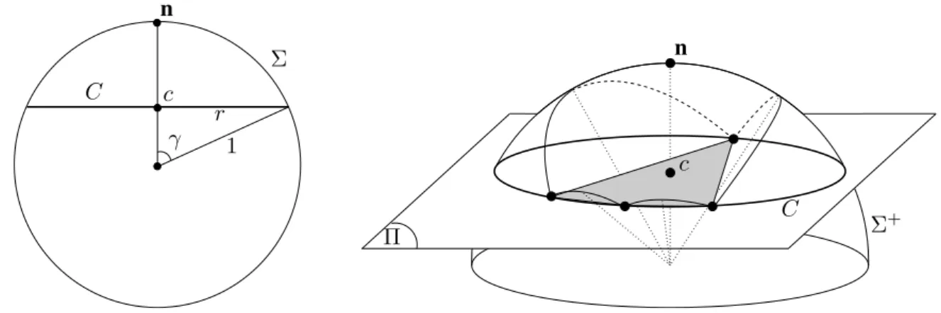
Let p be a point of S and µ a positive constant. We call Bp the closed ball centered at p of radius µ rch(S), and we set Dp = S∩ Bp.

Lemma 1.4 (Cocone)

If µ < π

2+π, then, for any q ∈ Dp, Dplies outside the double cone K(q) of apex q, of axis aligned with

n(p) and of half-angle π 2 −

µ 1−µ.

(33)

cB c_D D D0 _u _f v w

Proof. Let l be a line included in K(q), and l be a vector aligned with l such that n(p) · l ≥ 0. By definition of K(q), we have (n(p), l) < π

2 − µ

1−µ. Moreover, by the normal variation lemma 1.2, we have (n(p), n(q0₎₎_≤ µ

1−µ, for any q0 ∈ Dp. Thus, (n(q0),l) < π2 − µ 1−µ +

µ

1−µ = π2. Since this is true for any point q0 _{∈ Dp, l intersects Dp}_{at most once, by the line lemma 1.3. Hence, l ∩ D}_p₌_{q}. _¤

Let now f = (u, v, w) be a triangle whose vertices u, v and w belong to S. Let n(f) denote the unit vector orthogonal to f such that n(f) · n(u) ≥ 0. The next result is an adaptation of Lemma 7(a) of [6]. We recall its proof, for completeness.

Lemma 1.5 (Triangle Normal)

If the circumradius of f is at most µ rch(S), with µ < 1, and if the inner angle ˆu = ∠vuw is at least π 3,

then (n(f), n(u)) ≤ µ√3.

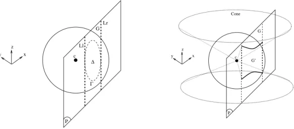
Proof. Let B and B0 _{denote the two balls of radius rch(S) tangent to S at u, D = B ∩ aff(f) and} D0 = B0_{∩ aff(f). We call cB}and cD the centers of B and D respectively. Moreover, rf _{≤ µ rch(S)} denotes the circumradius of f, and rD ≤ rch(S) denotes the radius of D and D0 (which have same radius, by a symmetry argument).

Let rf be fixed. Since the interiors of D and D0 _{do not intersect S, they contain no vertex of f.} Therefore, rDis maximized with respect to rf when v and w are farthest from u and lie on the boundaries of D and D0_{. Since we assumed that ˆu ≥} π

3, v and w are farthest from u when f is equilateral. It follows that rD ≤ rf √3.

In addition, according to the hypothesis, rf ≤ µ rch(S). We then have:

sin(n(f), n(u)) = sin(∠ucBcD)≤

d(u, cD) d(u, cB) = rD rch(S) ≤ µ √ 3 (1.1) ¤

(34)

1.2 Global properties

In this section, we review the main global properties of Del_|S(E)in the case where E is a loose ε-sample of S with sufficiently small ε. Let µ0 = 0.16and ν = 0.52. These two constants are set up so that the bounds in the following statements are as tight as possible. Throughout the section, E denotes a loose ε-sample of S. Let µ = ε/rch(S).

For any facet f of Del_|S(E), we call Bf the surface Delaunay ball of smallest radius that circum-scribes f. Let cf and rf denote respectively the center and radius of Bf. We set Df = S_{∩ Bf}.

Orientation convention 1.6 For any facet f ∈ Del(E) of circumradius less than (1 + ν)ε, we orient f

such that n(f) · n(uf) > 0, where uf is the vertex of f with largest inner angle (if it is not unique, we

choose any such vertex).

Notice that it is not necessary to orient all the facets of Del(E), because only those of circumradius less than (1 + ν)ε will be considered in the sequel. Among these are the facets of Del_|S(E), which are included in surface Delaunay balls of radius at most ε.

In Section 1.2.1 (Th. 1.7) we will show that, if µ ≤ µ0, then Del|S(E) is an oriented manifold without boundary. The proof does not rely on the fact that the surface S is smooth, therefore Theorem 1.7 will be used in Chapter 2 as well, for the nonsmooth case. However, we have to work under slightly more general hypotheses. Specifically, we prove that, if E is a loose ε-sample of S (for some ε which can be greater than µ0 rch(S)) satisfying the following assumption:

For any vertex v of Del_|S(E), there is a point pv ∈ S where S is differentiable, such that:

M1 For any q ∈ S ∩ B(v, ε), S ∩ B(v, ε) lies outside the double cone of apex q, of axis aligned

with n(pv)and of half-angleπ₂ − θ1.

M2 For any restricted Delaunay facet f incident to v, (n(f), n(pv))≤ θ2.

M3 For any Delaunay facet f incident to v, of circumradius less than (1+ν)ε, (n(f), n(pv))≤ θ3.

where θ1, θ2and θ3depend only on ε and verify: M4 2θ1+ θ2 < π₂.

M5 2 sin θ1< ν cos θ2. M6 sin θ1 < cos θ3.

then Del_|S(E)is an oriented manifold without boundary.

When S is smooth and µ ≤ µ0, for any vertex v of Del|S(E)we take pv = v, and we set θ1 = 1−µµ , θ2 = µ

√

3 + _1−2µ2µ and θ3 = (1 + ν) µ√3 + 2(1+ν) µ

1−2(1+ν) µ. By the cocone lemma 1.4, M1 is satisfied. Moreover, by the triangle normal lemma 1.5 and the normal variation lemma 1.2, M2 and M3 are satisfied as well. Finally, since µ ≤ µ0, M4, M5 and M6 are also satisfied. Therefore, Del|S(E)is an oriented manifold without boundary.

In Sections 1.2.2 and 1.2.3, we will prove that Del_|S(E)is isotopic to S and at Fréchet distance O(ε2₎from S, provided that µ ≤ µ0. The proofs use the fact that Del

|S(E)is a manifold, as guaranteed above. Moreover, they hold in a slightly more general setting. Specifically, we will show that, for any finite point set E ⊂ S and any subcomplex ˆS of Del|S(E)verifying:

(35)

I1 ˆS is a compact surface without boundary, consistently oriented by the orientation

conven-tion 1.6,

I2 ˆS has vertices on all the connected components of S,

I3 For any facet f of ˆS, Bf has a radius at most ε ≤ µ0rch(S), ˆ

Sis isotopic to S and at Fréchet distance O(ε2₎from S. Our arguments rely heavily on the fact that the surface S is smooth, hence the results cannot be used in Chapter 2, for the nonsmooth case. Nevertheless, the proofs of Chapter 2 will keep the same spirit.

The fact that ˆSis a subcomplex of Del_|S(E)(and not Del_|S(E)itself) will be instrumental in prov-ing the correctness of certain Delaunay refinement algorithms in several meshprov-ing applications. See Section 5.1 and Chapter 8.

1.2.1 Manifold

This section is dedicated to the proof of the following result:

Theorem 1.7 If E is a loose ε-sample of S, such that M1–M6 are satisfied, then Del_|S(E)is a compact

oriented surface without boundary.

In Section 1.2.1.1, we show that every edge of Del_|S(E)is incident to exactly two facets of Del_|S(E). In Section 1.2.1.2, we show that every vertex of Del_|S(E)is incident to exactly one cycle of facets of Del_|S(E). Such a cycle will be called an umbrella. These two properties imply that Del_|S(E)is a 2-manifold without boundary, because the relative interiors of the faces of Del_|S(E)are pairwise disjoint due to the fact that Del_|S(E)is a simplicial complex. Finally, in Section 1.2.1.3, we prove that the orientation convention 1.6 induces a valid orientation of Del_|S(E).

1.2.1.1 Edges

We need an intermediate result: Lemma 1.8 (Projection)

Under M1, M2 and M4, for any facets f, f0 _{of Del}

|S(E)with a common edge e, for any vertex v of e,

the orthogonal projections of f and f0onto T (p_v₎do not overlap, i.e. their interiors are disjoint. Proof. Let u be the second vertex of e. For convenience, we note B = Bf, r = rf the radius of Bf, and c = cf the center of Bf. Similarly, we call B0_{= B}

f0, r0 = r_f0, c0 = c_f0.

Since u and v are vertices of f and f0_{, ∂B and ∂B}0 _{have a non-empty intersection. Let P be the} radical plane of B, B0. P contains ∂B ∩ ∂B0, and therefore also u and v. Let w be the third vertex of f, and w0 _{be the third vertex of f}0_{. P is perpendicular to the line (c, c}0_{). On one side of P , B is included} in the interior of B0, whereas on the other side of P , B0is included in the interior of B. Since B and B0 are Delaunay balls, B cannot contain w0 _{and B}0 _{cannot contain w. Hence, w and w}0 _{cannot lie on the} same side of P .

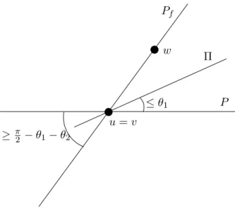
Let Π be the plane that contains u, v and n(pv). Since Π is orthogonal to T (pv), its orthogonal projection onto T (pv)is a line containing the projection of e. Hence, to prove that the projections of f and f0 _{onto T (pv}₎_{do not overlap, it suffices to show that w and w}0_{lie on different sides of Π.}

(36)

PSfrag replacements Pf Π P T (pv) u = v w ≤ θ1 ≥ π 2 − θ1− θ2

P and Π intersect each other along the line (u, v). We define an oriented frame in R3such that P is the horizontal plane and that w lies above P . The line (u, v) = P ∩ Π is then horizontal. We will show that w lies above Π while w0 _{lies below, which will conclude the proof of the lemma.}

Since r ≤ ε and r0 _{≤ ε, c and c}0_{belong to S ∩ B(v, ε). Thus, by M1 (applied with q = c), the angle} between n(pv)and the line (c, c0₎is at least π

2 − θ1. This implies that the angle between n(pv)and P is at most θ1, since P is orthogonal to the line (c, c0₎_{. Hence, the angle ∠ΠP between planes Π and P is} bounded by θ1. In addition, by M2 we have (n(f), n(pv))≤ θ2. It follows that the angle between n(f) and P is at most θ1+ θ2, or equivalently, that the angle ∠PfP between the supporting plane of f and P is at least π

2 − θ1− θ2. By M4, this quantity is greater than θ1, which means that ∠PfP is greater than ∠ΠP . Hence, w lies above Π – see Fig. 1.3. By the same arguments, w0 lies below Π, which concludes

the proof of the lemma. ¤

Remark 1.9 Observe that the proof of the projection lemma still holds if B and B0 _{are two surface}

Delaunay balls circumscribing the same facet f = f0. Hence, B_f is the only surface Delaunay ball that

circumscribes f. Equivalently, the Voronoi edge V(f) dual to f intersects S only once. Moreover, the vertices of V(f) belong to distinct connected components of R3_{\ S since otherwise a small perturbation}

of V(f) would intersect S ∩ Bf twice, hereby contradicting the projection lemma 1.8 (with f = f0). From the projection lemma 1.8, we deduce the following result:

Lemma 1.10 Under M1, M2 and M4, every edge of Del_|S(E) is incident to exactly two facets of Del_|S(E).

Proof. Let e be an edge of Del_|S(E). By definition, e is incident to a Delaunay facet f whose dual Voronoi edge V(f) intersects S. V(f) is an edge of ∂V(e), the boundary of the Voronoi facet dual to e. By Remark 1.9, the vertices of V(f) lie in distinct connected components of R3_{\ S. Hence, ∂V(e)}

(37)

intersects S at least twice, since it is a topological circle that intersects two distinct connected coponents of R3_{\ S. As a consequence, e is incident to at least two facets of Del}

|S(E).

In addition, e cannot be incident to more than two facets of Del_|S(E). Indeed, by the projection lemma 1.8, the projections onto T (pv)(where v is any vertex of e and pv is defined as in M1, M2, M4) of the restricted Delaunay facets incident to e pairwise do not overlap, thus they must lie on different sides of the line supporting the projection of e.

In conclusion, the number of facets of Del_|S(E)incident to e is two. ¤

1.2.1.2 Umbrellas

Consider a vertex v of Del_|S(E). Since every edge of Del_|S(E)incident to v has two incident facets of Del_|S(E), the star of v in Del_|S(E)consists of one or more cycles of facets, called umbrellas. Each umbrella is a triangulated topological disk. All umbrellas of v have v in common, but two distinct umbrellas have distinct edges and facets. We call ¯v the orthogonal projection of v onto T (pv).

Lemma 1.11 Under M1, M2, M3, M5 and M6, v has exactly one umbrella.

Proof. Let U be an umbrella incident to v. We call ¯U its orthogonal projection onto T(pv). Claim 1.11.1 ¯v belongs to the interior of ¯U.

Proof. Let us assume the contrary. Then U has a silhouette edge [v, u] whose projection onto T(pv) belongs to the boundary of ¯U. Since, by lemma 1.10, [v, u] is incident to two facets of U, these two facets project onto the same side of the line supporting the projection of [u, v], therefore they operlap, which contradicts the projection lemma 1.8. This proves the claim. ¤

Assume now, for a contradiction, that v has several umbrellas. Let U and U0 _{be two consecutive} umbrellas (recall that two umbrellas of v intersect only in v). Let T be the set of tetrahedra of Del(E) incident to v that lie between U and U0_.

Let l be a line parallel to n(pv)and passing through a point of Del_|S(E)very close to v. We orient l as n(pv). Let T = (t1, . . . , ts)be the sequence of tetrahedra of T that are intersected by the oriented line l, and let F = (f0, . . . , fs)be the facets of T pierced by l. We assume without loss of generality that l does not pass through an edge of one of the ti. By definition, f0 ∈ U and fs⊂ U0_{are facets of Del}

|S(E). We rename them f and f0 _{respectively, and call c and c}0_{the centers of their surface Delaunay balls. Let} c1, . . . , csbe the centers of the Delaunay balls circumscribing t1, . . . , ts, and γ be the polygonal chain γ = c, c1, . . . , cs, c0. For convenience, we write c = c0 and c0 = cs+1. Clearly, γ is a path in the 1-skeleton graph of Vor(E).

Claim 1.11.2 γ is monotone with respect to the oriented line l.

Proof. l intersects tibefore ti+1, for i = 1, . . . , s − 1. Thus, n(pv)· ni > 0, where niis the unit normal vector of fi, oriented from tito ti+1. Since tiand ti+1are Delaunay tetrahedra, we have ni= ci+1−ci