HAL Id: hal-01878100
https://hal.inria.fr/hal-01878100
Submitted on 20 Sep 2018
HAL is a multi-disciplinary open access
archive for the deposit and dissemination of
sci-entific research documents, whether they are
pub-lished or not. The documents may come from
teaching and research institutions in France or
abroad, or from public or private research centers.
L’archive ouverte pluridisciplinaire HAL, est
destinée au dépôt et à la diffusion de documents
scientifiques de niveau recherche, publiés ou non,
émanant des établissements d’enseignement et de
recherche français ou étrangers, des laboratoires
publics ou privés.
A Generalized Digraph Model for Expressing
Dependencies
Pascal Fradet, Xiaojie Guo, Jean-François Monin, Sophie Quinton
To cite this version:
Pascal Fradet, Xiaojie Guo, Jean-François Monin, Sophie Quinton. A Generalized Digraph Model
for Expressing Dependencies. RTNS ’18 - 26th International Conference on Real-Time Networks
and Systems, Oct 2018, Chasseneuil-du-Poitou, France. pp.1-11, �10.1145/3273905.3273918�.
�hal-01878100�
A Generalized Digraph Model
for Expressing Dependencies
Pascal Fradet
1, Xiaojie Guo
1,2, Jean-François Monin
2and Sophie Quinton
11
Univ. Grenoble Alpes, Inria, CNRS, Grenoble INP, LIG, F-38000 Grenoble France 2
Univ. Grenoble Alpes, CNRS, Grenoble INP, VERIMAG, F-38000 Grenoble France
ABSTRACT
In the context of computer assisted verification of schedulability analyses, very expressive task models are useful to factorize the correctness proofs of as many analyses as possible. The digraph task model seems a good candidate due to its powerful expressivity. Alas, its ability to capture dependencies between arrival and execution times of jobs of different tasks is very limited.
We propose here a task model that generalizes the digraph model and its corresponding analysis for fixed-priority scheduling with limited preemption. A task may generate several types of jobs, each with its own worst-case execution time, priority, non-preemptable segments and maximum jitter. We present the correctness proof of the analysis in a way amenable to its formalization in the Coq proof assistant.
Our objective (still in progress) is to formally certify the analysis for that general model such that the correctness proof of a more specific (standard or novel) analysis boils down to specifying and proving its translation into our model. Furthermore, expressing many different analyses in a common framework paves the way for formal comparisons.
1
INTRODUCTION
The need for computer assisted verification of analysis techniques in the area of real-time systems has been recognized by the research community. The work presented here is part of an effort to con-tribute to Prosa [1], a library of definitions and proofs for real-time schedulability analyses using the Coq proof assistant [2]. Formal verification requires an important human effort, so making proofs general, generic, and/or reusable is of great importance.
Our goal is to factorize the formal certification of existing Re-sponse Time Analyses (RTAs) for fixed-priority policies. There exists a wide variety of task models and analyses for such policies. However, most of these models are incomparable and very few can describe dependencies between arrival and/or execution time of different jobs. The Digraph Real-Time Task (DRT) model [21] seems a good candidate for modeling intra-task dependencies, but its ability to capture dependencies between different tasks is very limited. It cannot, for example, capture Tindell’s offset model [25].
Permission to make digital or hard copies of all or part of this work for personal or classroom use is granted without fee provided that copies are not made or distributed for profit or commercial advantage and that copies bear this notice and the full citation on the first page. Copyrights for components of this work owned by others than the author(s) must be honored. Abstracting with credit is permitted. To copy otherwise, or republish, to post on servers or to redistribute to lists, requires prior specific permission and /or a fee. Request permissions from [email protected].
RTNS ’18, October 10–12, 2018, Chasseneuil-du-Poitou, France
© 2018 Copyright held by the owner/author(s). Publication rights licensed to ACM. ACM ISBN 978-1-4503-6463-8/18/10. . . $15.00
https://doi.org/10.1145/3273905.3273918
In this paper, we propose a task model that generalizes the DRT model and its corresponding RTA, with the restriction that we con-sider discrete time while some results about DRT apply to dense time. A task may generate several types of jobs, each with its own worse-case execution time (WCET), priority, non-preemptable seg-ments and jitter. Our model can capture dependencies between jobs of the same task as well as jobs of different tasks. We focus on fixed-priority scheduling policies and our model can encompass preemptive and nonpreemptive models, as well as limited preemp-tion. Despite being much more general, the RTA for our model is not significantly more complex than the original one. Also, it underlines similarities between existing analyses, in particular the analysis for the DRT model and Tindell’s offset model.
For the time being, the proof of the RTA of the general model within the Coq proof assistant is not yet complete. When it is certi-fied, the design and proof of a more specific (standard or novel) RTA will boil down to specifying and proving its translation into our model. Furthermore, expressing many different RTAs in a common framework paves the way for formal comparisons and generaliza-tions (e.g., design of novel RTAs).
To summarize, the main contributions of this paper are: (1) A general task model which encompasses complex
depen-dencies between jobs and tasks; (2) A RTA for that model;
(3) A correctness proof of that RTA amenable to its formalization in Coq and applicable to other task models.
The paper is structured as follows. Section 2 introduces the sys-tems we consider and provides basic definitions to describe their runtime behavior. Section 3 presents the syntax and semantics of our task model and Section 4 provides intuition about its expressiv-ity. Section 5 presents the associated RTA and Section 6 sketches its correctness proof. Section 7 puts the contribution of this paper into the perspective of our broader project of a Coq library of schedula-bility results. We discuss related models in Section 8 and conclude in Section 9.
2
SYSTEM BEHAVIOR
We target concrete systems implemented as a set of tasks executing on a uniprocessor. The execution proceeds according to ajob-level fixed-priority limited preemptive (JFPLP) scheduling policy. A JFPLP scheduler arbitrates between jobs competing for processor time by choosing the highest priority job, but it can only preempt a running job at some predefined execution point. In other words, each job is decomposed into non-preemptable segments. This model subsumes the Fixed Priority Preemptive (FPP) and Fixed Priority Non-Preemptive (FPNP) policies, and permits mixed policies [3]. A task can generate different types of jobs. Jobs of the same type have similar properties, in particular they have the same priority.
2.1
Definition of system behavior
We assume a set T of type names (types, for short). Each type entails a number of characteristics that are described in Section 2.
Definition 1 ( Job⋆1). A jobȷ is specified by: • itstype v(ȷ) ∈ T;
• itspriority p(ȷ) ∈ N inherited from its type; A greater number means a higher priority.
• itsarrival time a(ȷ) ∈ N;
• itsjitter j(ȷ) ∈ N (also called release delay);
• a vector⃗c(ȷ) = ⟨c1, . . . , cs⟩,ci ∈ N+, of durations
correspond-ing to thecost (i.e., execution time) of each non-preemptable seg-ment.
Thecost (or required service time) of a job ȷ as above is c(ȷ) = P
1≤i ≤sci. Therelease time ofȷ is r(ȷ) := a(ȷ) + j(ȷ).
We do not exclude different jobs from having the same parame-ters, but we assume that they can be distinguished (e.g., through an identifier). We also assume that the set of jobs is partitioned intotasks. The behavior of a system is described using a set of executions defined by ajob arrival sequence and a schedule.
Definition 2 ( Job arrival sequence⋆). A job arrival sequence is a functionρ mapping any time instant t to a finite (possibly empty) set of jobsρ(t ) such that ȷ ∈ ρ(t ) iff a(ȷ) = t.
Note that once the set of jobs and the functiona are given, ρ is uniquely determined. A jobȷ completes when it has received as much service time as it required, which is determined by the schedule. We denote its completion time byend(ȷ). The response time ofȷ is defined as RTȷ := end(ȷ) − a(ȷ). From its release time and until completion, a job is said to bepending.
Definition 3 (Schedule, JFPLP schedule⋆). A schedule is a par-tial functionσ which maps any time instant t to the job (if any) that is scheduled (i.e., receives service) att . A job ȷ can be scheduled only when it is pending.
AJFPLP schedule is a schedule such that the job that is scheduled is: either the job that is already executing one of its non-preemptable segments, or a job that has the highest priorityh among pending jobs. If there are several pending jobs with priorityh, a task is arbitrarily selected among those with such jobs; the chosen job is then the first released job with priorityh in this task (FIFO policy).
2.2
Additional definitions and notations
In the following, we will need additional definitions and notations, which we introduce here.
Definition 4 ( Job release sequence). Letρ be a job arrival se-quence. The corresponding job release sequence, written ˆρ, is de-fined as ˆρ(t ) := {ȷ | ȷ ∈ ρ(t′) ∧ t = t′+ j(ȷ)}. We have ȷ ∈ ˆρ(t) iff r(ȷ) = t.
We will occasionally write arrival (or release) sequences as lists of sets of jobs. For instance, [(t1, {ȷ1, ȷ2}), (t2, {ȷ3}), . . .] denotes a
sequenceρ such that ρ(t1) = {ȷ1, ȷ2},ρ(t2) = {ȷ3} andρ(t ) = ∅ for
allt absent from the list.
1The definitions and lemmas decorated with a star have been formalized in Coq/Prosa,
see discussion in Section 7.
Therestriction of a job arrival sequenceρ to a time interval [t1, t2[ is denotedρ/[t
1,t2[
. The same applies to job release sequences. Definition 5 (Workload⋆). Let ρ be a job arrival sequence and V a set of job types. The workload wlV , ρ of jobs with type inV in a time interval [t1, t1+ ∆[ is the cumulative cost (i.e., required service time) of such jobs released in that interval. Formally,
wlV , ρ(t1, ∆) :=
X
ȷ:v ∈V t1≤r( ȷ)<t1+∆
c(ȷ) (1)
Definition 6 (Service time⋆). Let σ be a schedule and V a set of job types. Theservice timeserv
V ,σreceived by jobs with type in V in a time interval [t1, t1+ ∆[ is servV ,σ(t1, ∆) := X t ∈[t1,t1+∆[ v(σ (t )) ∈ V 1 (2)
Our RTA analysis (Section 5) is based on the concept of busy window which we formally introduce now. The following defini-tions are implicitly parameterized by a job arrival sequenceρ and a scheduleσ .
Definition 7 (Level-p quiet time⋆). An instant t is said to be alevel-p quiet time if all jobs of priority higher than or equal to p released strictly beforet have completed at t .
Definition 8 (Level-p busy window⋆). A time interval [t1, t2[
is said to be alevel-p busy window if: (1) t1andt2are level-p quiet times;
(2) there is no level-p quiet time in ]t1, t2[; and
(3) at least one job with a priority higher than or equal top is released in [t1, t2[.
The last condition excludes degenerate cases of busy windows in which no job is scheduled. Since several jobs with the same type may be released in the same busy window, we introduce (again in a way similar to the state of the art) the additional concept of queueing prefix.
Definition 9 (Queueing prefix⋆). The q-th queueing prefix of jobs of typev in a level-p busy window [t1, t2[ is the time interval
[t1, tq] wheretqis the instant at which the last non-preemptable
segment of theq-th job of type v receives its first service (i.e., is scheduled for the first time).
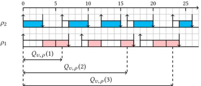
Example 1. Figure 1 presents a job arrival sequenceρ (split into ρ1andρ2) in a system made of two tasks. One task produces jobs of
typev, priority 1, jitter 0 and segments ⟨2, 2⟩ and two consecutive arrival times of its jobs are separated by at least 9 time units. The other task produces jobs of priority 2. The three first queueing prefixes of jobs of typev in the level-1 busy window [0, 27[ are Qv, ρ(1), Qv, ρ(2) and Qv, ρ(3).
3
GENERALIZED DIGRAPH TASK MODEL
Our task model, called thegeneralized digraph (Gd) model, is an ex-tension of the digraph model [21] with job level priorities, possibly null inter-arrival times, jitter and non-preemptable segments.
Qv, ρ(1) Qv, ρ(2) Qv, ρ(3) ρ1 ρ2 0 5 10 15 20 25
Figure 1: Queueing prefixes of jobs of typev.
3.1
Syntax
A system consists of a set ofn independent tasksΣ := {G1, . . . , Gn},
each task being specified by a graphGi := (Vi, Ei) where: •Viis a set of vertices representing different job types; • Ei is a set of edges such that an edge connecting two vertices v1andv2ofViis labeled with a durationd(v1,v2) ∈ N representing
the minimum inter-arrival time between jobs of typesv1andv2.
A job typev is characterized by the following parameters2: • P(v) ∈ N defines the priority of jobs of type v;
• J(v) ∈ N specifies the maximum jitter (i.e., delay between arrival and release time) for jobs of typev;
• ⃗C(v) = ⟨C1, . . . , Cs⟩ is a vector specifying the maximum cost
of each non-preemptable segment of jobs of typev; C(v) = Ps
i=1Ci
defines the maximum cost of jobs of typev.
The sets of verticesViare assumed to be disjoint (i.e., tasks activate jobs of different types). The set of vertices of the complete system is denoted byVΣ= Sn
i=1Vi. For simplicity and to improve readability, we assume in this paper that the jitter isconstrained3: the jitter of any vertexv ∈ VΣ is smaller than or equal to the minimum inter-arrival time labeled on any edge going out ofv.
In contrast with the standard digraph task model, null inter-arrival times are allowed. We however disallow tasks (i.e., graphs) that contain null cycles (which would permit an infinite nomber of job arrivals at the same instant). This is easily verified statically.
In the following, we notehep(p), hp(p), ep(p), lp(p) the sets of vertices of the system whose priorities are equal or higher, higher, equal and lower thanp, respectively.
Example 2. The graphGerepresented in Figure 2 defines a task with three vertices (i.e., three types of jobs). Vertexu is decorated with the triplet(⟨1, 1⟩, 0, 1) where ⟨1, 1⟩ indicates that jobs of this type can be preempted at each instant (segments of length 1) and their maximum cost is 2= 1 + 1; their maximum release jitter is 0 and their priority is 1. Similarly, jobs of typev have a maximum cost of 5 and cannot be preempted, their maximum jitter and priority are 3 and 2, respectively. Jobs of typew have a maximum cost of 8 and can be preempted after at most 4 time units of execution.
3.2
Task-level and system paths
As a graph, a taskGi = (Vi, Ei) specifies a set of (possibly infinite) paths, i.e., sequences of vertices ofGisuch that(vj,vj+1) ∈ Ei. Note
2
The RTA presented in this paper does not rely ondeadlines and we omit this parameter.
3
The extension to arbitrary jitter is discussed in Section 4.3.
u v w (⟨1, 1⟩, 0, 1) (⟨5⟩, 3, 2) (⟨4, 4⟩, 0, 1) 8 16 10 20
Figure 2: A graphGespecifying a task with 3 types of jobs
that a task will typically have cycles, thus specifying an infinite set of paths, some of them infinite. In the following, we sometimes refer to paths of tasks as task-level paths for clarity.
Example 3. In Figure 2, [u, v, u, w, v], [w, v, u, v, u], and the infinite sequenceX = [u,v, X] are paths of Ge, but [u, v, w] is not. Definition 10 (System path). Asystem path of systemΣ is a set π := {π1, . . . , πn} such that for eachi, πiis a task-level path of task
GiinΣ. The set of system paths of Σ is denoted ΠΣ.
We will use later the following operations on task-level paths. • The functionlen returns the sum of all minimum inter-arrival times on the edges of a finite path. Formally:
len([v1,v2, . . . ,vk]) :=
X
1≤j <k
d(vj,vj+1)
• The functionpre∆(πi) returns the longest prefix πpofπisuch thatlen(πp) < ∆. A variant, written prevn(πi), returns the prefix of πi up to then-th occurrence of vertex v in πi.
• We writelennv(πi) for len(prenv(πi)) which returns the sum of
all minimum inter-arrival times between the first vertex and the n-th occurrence of vertex v in πi.
• The functioncost(seq) returns the sum of the maximum cost of all vertices in a vertex sequenceseq.
• The filter function |π |V returns the vertex sequence obtained fromπ where all vertices not belonging to V have been filtered out.
3.3
Semantics
The semantics of a systemΣ := {G1, . . . , Gn} is given by the set
of arrival sequences that areconsistent with a system path ofΣ. Consistency between an arrival sequence and a system path ensures that jobs in the sequence satisfy the constraints imposed on them by their type and that the order and timing of job arrivals is compatible with the constraints specified on the edges of the graphsGi.
Definition 11 (Consistency of an arrival sequencew.r.t. a path). An arrival sequenceρ is consistent with a task-level path πi = [v1,v2, . . .], which is denoted ρ ∼ π, iff there exists a flattening
4
[(t1, ȷ1), (t2, ȷ2), . . .] of ρ such that for all k:
• ȷkis consistent withvk,i.e., : – v(ȷk) = vk;
– p(ȷk) = P(v); – j(ȷk) ≤ J(vk); and
4
For example, the arrival sequence[(t1, { ȷ1, ȷ2}), (t3, { ȷ3})] can be flattened into
either[(t1, ȷ1), (t1, ȷ2), (t3, ȷ3)] or [(t1, ȷ2), (t1, ȷ1), (t3, ȷ3)]. 3
– ⃗c(ȷk) = ⟨c1, . . . , cs⟩ ∧ ⃗C(vk) = ⟨C1, . . . , Cs⟩ ∧ci ≤Ci, i = 1. . . s.
•d(vk,vk+1) ≤ tk+1−tk
The definition naturally extends to system-level paths.
We writeρ ∼Σ to denote that an arrival sequence ρ is consistent with a system path inΠΣ.
4
EXPRESSIVITY OF THE GD MODEL
In this section, we show how a variety of existing task models can be expressed using the Gd model. We also hint at extended or new models that could be defined as Gd and analyzed by our proposed RTA.
4.1
Models without task dependencies
The Gd model can easily emulate many kinds of arrival models. Obviously, a simple sporadic task whose jobs are of typev and with a minimum inter-arrival timep is represented by a single vertex v and self-loop labeled with p. A periodic task of period p can be represented by the same Gd task. Of course, this Gd task represents many more consistent job arrival sequences but the worst case analyzed by the RTA is precisely the periodic sequence.
Arrival curves [24] represent more expressive arrival models. For instance, the minimal distance functiond
−
(a) returns the smallest time interval that may containa+ 1 occurrences of a job. This func-tion must be super-additivei.e.,d
−
(a) +d−
(b) ≤ d−
(a +b). In general, an arrival curve may have an infinite description in terms of Gd task (e.g.,d
−
(a) = a2
is super-additive and describes ever growing inter-arrival times). However, such functions5are usually given by a collection of values from 1 to some constantk. Then, the anal-ysis uses the minimal super-additive extension (e.g., the smallest function compatible withd
−
(1), . . . ,d−
(k)). Such super-additive clo-sures can be represented faithfully by a Gd task. Whend
− is convex (i.e.,d − (x + 1) + d− (x − 1) − 2d−
(x) ≥ 0) then the minimal super-additive extension is periodic and∀x = qk +r,d
−
(x) = qd−
(k) +d−
(r ). The corresponding Gd task is then made of a cycle ofk vertices v0, . . . ,vk−1where the minimum inter-arrival time decorating each
edge isd(vi,v(i+1) mod k) = d
−
((i + 1) modk) − d−
(i).
Example 4. Consider, for instance, the arrival curve specified byd
−
(1) = 2,d−
(2) = 5,d−
(3) = 10,d−
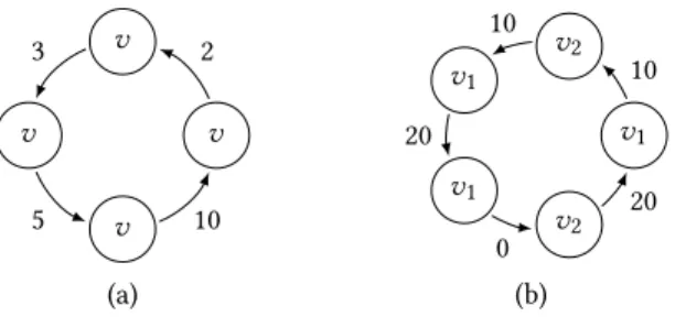
(4) = 20 which specifies that 2 (resp. 3, 4, and 5) jobs cannot arrive in less than 2 (resp. 5, 10 and 20) time units. The corresponding Gd task is given in Fig.3 (a).
For non convex functions, it has been shown that their minimal super-additive extensions are pseudo-periodic functions [10] which can also be represented by a finite Gd task.
4.2
Models with job and task dependencies
As a generalization of digraphs, the Gd model can of course express all task models with intra-task dependencies that standard digraphs can. Let us cite, the multiframe model [18] and its generalized version [6], the recurring branching [7] or recurring RT [8] models, the non cyclic RT [4] and digraph model (DRT) [21].
Allowing job-level fixed priorities and null minimal inter-arrival times allows the Gd model to model inter-task dependencies
5 By defaultd − (0) = 0 v 2 v 3 v 5 v 10 v1 10 v2 10 v1 20 v1 0 v2 20 (a) (b)
Figure 3: Gd representing (a) an arrival curve model and (b) a transaction with offsetsa la Tindell)
(e.g., fixed timing relation among tasks), e.g., the offset model of Tindell [25] (which cannot be represented in the standard DRT model).
In Tindell’s model, a system is made of a set of independent transactions{Tr1, . . . , Trn}. Each transactionTriconsists of a set
of periodic tasks with offsetsTri := {. . . ,τi,k, . . .} where each task τi,k has its own WCET, period, offset, priority, and deadline. A transaction and its set of periodic tasks with offsets can be rep-resented within a single Gd task. It is sufficient to compute the hyper-period of the transaction and to build the circular Gd task representing the inter-arrival time (which may be null) between arrivals of the different jobs in the hyper-period. The periods and offsets are represented by inter-arrival times. The WCET, priority and deadline of tasks are represented by the corresponding vertices. Example 5. Consider, for instance, a transactionTr with two periodic tasks with jobs of typev1 andv2, with periods 20 and
30 and with offsets 5 and 15. The hyper-period is 60 and tak-ing the first arrival ofv1 as the time origin, the arrival times are [(v1, 0), (v2, 10), (v1, 20), (v1, 40), (v2, 40), (v1, 60)]. The
trans-actionTr is represented by the Gd task in Fig.3 (b). Its worst job arrival sequencew.r.t. the RTA is exactly the job arrival sequences ofTr.
Shared resources, which entail inter-tasks dependencies, is a com-mon issue in hard real-time systems. Abdullah et al. [3] addressed this problem using DRT by allowing two kinds of vertices : pre-emptable (tasks) and non-prepre-emptable (resources). They proposed an extension of the RTA to take into account these two kinds of ver-tices. Using the Gd model, this is directly modeled using segments with always preemptable vertices for tasks and non-preemptable ones for resources.
Rendez-vous mechanisms, another kind of inter-task depen-dencies, have been expressed using an extension of digraphs (SDRT) [17]. We believe that the encoding of such inter-task syn-chronization is possible in Gd tasks but the exact encoding as well as its complexity remain to be investigated.
4.3
Beyond existing models
All these features, including jitter, can be combined to express and analyse new task models. For instance, non-preemptable segments and jitter have not been considered into intra-task dependencies task models (e.g., MF, GMF, RB, RR, DRT) nor do Tindell’s model consider intra-task dependencies (e.g., if a transaction could be a set of MF tasks instead of simple periodic tasks). Since all these
models can be expressed as the Gd model, they can be analyzed using the RTA described next.
Note that the following RTA targets the Gd model with con-strained jitters. Because any Gd task with arbitrary jitters can be transformed into a Gd task with constrained jitters remaining the same worst case analyzed by the RTA. For instance, a sporadic task of the minimum inter-arrival time 10 and jitter 22 represented by G can be transformed into G’ with jitter 0 in Fig. 4.
v 10 (⟨3, 3⟩, 22, 1) v 0 v v v (⟨3, 3⟩, 0, 1) 0 8 10 (G) (G’)
Figure 4: Encoding of arbitrary jitter
5
RESPONSE TIME ANALYSIS OF GD SYSTEMS
The objective of RTA is to bound, as tightly as possible, the worst-case response time of each vertex (job type)v, defined as the maxi-mum response time among all jobs of typev occurring in all arrival sequences consistent with each possible system path. Formally,
wcrt(v) := max{RTȷ |ȷ : v ∧ ∃π ∈ΠΣ, ∃ρ ∼ π, ȷ ∈ ρ}
In this section, we present the overall structure of the analysis that we propose for Gd systems. We suppose given a vertexv, with priorityp, of a task Gi ∈Σ and focus on upper bounding its worst-case response time.
Our analysis relies on a path-specific analysis of level-p busy windows, hence the following definition (implicitly parameterized as before by a job arrival sequenceρ).
Definition 12 (Busy window path). A level-p busy window [t1, t2[ is said to berepresented by the shortest system pathπ such
that ˆρ/
[t1,t2[∼π , and any extension of it.
The shortest path representing a busy window [t1, t2[ is the path
obtained after restricting the job release sequence to [t1, t2[. In
other words, a busy window path is an abstraction of a level-p busy window. Equipped with these notions, the general principle of our RTA analysis can now be presented.
5.1
Overall structure of the RTA of Gd systems
The RTA of a vertexv with priority p, of task Gi, consists in ana-lyzing a set of paths such that all possible level-p busy windows are represented by one path in the set. The methodology to bound the worst-case response time of jobs of typev is thus as follows. Step 1: Derive a set of system pathsΠv
Σ such that any possible level-p busy window (for any arrival sequence and schedule consistent with any system path inΠΣ) is represented by one path inΠv
Σ.
Step 2: For each system pathπ ∈ Πv
Σ:
a) Compute an upper boundBWp,π+ on the length of any level-p busy window represented by π ;
b) Derive fromπi(the task-level path ofGiinπ ) and BWp,π+ an upper boundq+
v,πi,BWp, π+
on the number of jobs of type v released in any level-p busy window represented by π ; c) Compute, for eachq ≤ q+
v,πi,BWp, π+
, an upper bound Qv,π+ (q) on the length of the q-th queueing prefix of jobs
of typev in any level-p busy window represented by π ; d) For each q ≤ q+
v,πi,BWp, π+
, compute a lower bound θv,π− i(q) on the (possibly negative) time difference
be-tween theq-th arrival of a job of type v in in any level-p busy window represented byπ and the start of that busy window;
e) Based on the above, compute an upper boundRTπ+(v) on the worst-case response time of any job of typev in any level-p busy window represented by π .
Step 3: Finally, compute an upper boundRT+
Σ(v) on wcrt(v).
In the following subsection, we provide the formulas used for the computations associated with each step of the methodology that we just presented, along with some intuition of where they come from. The proof of correctness of the computed values is presented in Section 6.
5.2
Step-by-step RTA of Gd systems
Our RTA relies on an upper bound on the workload of a set of jobs in any level-p busy window by the workload for the path in Πv
Σthat represents it, where the workload of a given set of verticesV ⊆ VΣ for a system-level pathπ := {π1, . . . , πn} ∈ΠvΣand a duration∆ is
wlV ,π+ (∆) := n X x=1 wl+V ,π x(∆) (3) with wl+ V ,πx(∆) := cost(|pre∆+J(fst(πx))(πx)|V)
We will show (see Lemma 2 in Sec. 6) that the workload of a set of verticesV ⊆ VΣfor any prefix of length∆ of a level-p busy window represented by a system pathπ is upper bounded by wl+
V ,π(∆).
Step 1: ComputingΠv
Σ—see Theorem 1 in Sec. 6
LetΠvx(∆) denote the set of paths πxof taskGx ∈Σ which • are the longest paths fitting in∆ + J+x, that is, such that len(πx) ≤ ∆ + J+x and for all valid suffixess, len(πx·s) > ∆ + J+x; whereJ+xrepresenting the largest release jitter amongVx.
• if the vertex under studyv belongs to Gi then we consider only pathsπxwith occurrences ofv.
With this notion of path, we compute a sufficiently large du-ration which can bound the length of any level-p busy window. That duration is the least positive fixed point, writtenWk, of the following equation ∆ = N + n X x=1 max πx∈Πvx(∆) {wl+hep(p),π x(∆)} (4)
withN denoting the greatest non-preemptable segment in the sys-tem. At each iteration, the greatest workload among all possible paths within∆ is selected. The obtained fixed point is clearly an upper bound on the duration of any possible busy window. There-fore, to boundwcrt(v), it is sufficient to examine all the following
combinations, ΠvΣ:= n
×
x=1Π v x(Wk) (5) where×
nx=1denotes the Cartesian product of all paths of length bounded byWkfor then tasks. Thus, any level-p busy window can be represented by (possibly a prefix of ) a path inΠv
Σ. Step 2: Computing upper bounds for each path inΠv
Σ
We now show how to computeBWp,π+ ,q+
v,πi,BWp, π+
,Qv,π+ (q) andθv,π−
i(q) for a given system path π := {π1, . . . , πn} ∈ΠvΣ.
a)ComputingBWp,π+ — see Theorem 2 in Sec. 6
Having non-preemptable segments implies that vertices inlp(p) may execute within a level-p busy window. Still, the definition of a level-p busy window implies that:
• at most one non-preemptable segment of a vertex inlp(p) can execute in a level-p busy window; and
• such a segment (if it exists) must have started its execution before the beginning of the level-p busy window.
As a result, the maximum duration that vertices inlp(p) can execute in a level-p busy window is upper bounded by:
Bp:= max
vx∈lp(p)
C ∈⃗C(vx)
(C − 1) (6)
with the convention thatBp := 0 if lp(p) = ∅. Now, let BWp,π+ be the least positive fixed point of the following equation:
∆ = Bp+ wl+hep(p),π(∆) (7) ThenBWp,π+ is an upper bound on the length of any possible level-p busy window represented byπ .
Note that it may be pessimistic to useBpto bound the workload fromlp(p) because the largest non-preemptable segment among lp(p) may not contribute to any level-p busy window represented byπ . On the other hand, it reduces the complexity of the analysis and simplifies its correctness proof6.
b)Computingq+
v,πi,BWp, π+
Definition 12 implies that the number of jobs of typev in a busy window is equal to the number ofv in its representing path. In addition, sinceBWp,π+ is an upper bound on the length of any possible level-p busy window represented by π , let q+
v,πi,BWp, π+
be the number of verticesv in the prefix preBW+
p, π+J(fst(πi))(πi) of
pathπi, thenq+
v,πi,BWp, π+
is an upper bound on the number of jobs of typev released in any level-p busy window represented by π . c)ComputingQv,π+ (q) — see Theorem 3 in Sec. 6
Theq-th queueing prefix of jobs of type v in a level-p busy window represented byπ spans the execution of:
• at most one non-preemptable segment from a vertex inlp(p) which started before that busy window;
• all jobs of taskGi with the same priority asv released during the prefix, up to theq-th job of v in πi (minus the cost of its last segment);
6An exact analysis would require considering up ton + 1 different critical instants for
a system withn tasks.
• the jobs of vertices fromGiinhp(p) released during the prefix; and
• the jobs of vertices inhep(p) released during the prefix, except those fromGi.
LetQv,π+ (q) be the least positive fixed point of the following equa-tion:
∆ = Bp
+ wl+ep(p)∩Vi,π(lenqv(πi) + 1) − last(⃗C(v)) + 1
+ wl+hp(p)∩Vi,π(∆) + wl+hep(p)\Vi,π(∆)
(8)
wherelast(⃗C(v)) is the maximum cost of the last segment ofv. Then, Q+v,π(q) is an upper bound on the length of the q-th queueing prefix
of jobs of typev in any possible level-p busy window represented byπ .
d)Computingθv,π−
i(q) — see Theorem 4 in Sec. 6
For eachq ≤ q+
v,πi,BWp, π+
, a lower bound on the duration be-tweent1and theq-th arrival of jobs of type v in any possible level-p busy window represented byπ is:
θv,π− i(q) := lenqv(πi) − J(fst(πi)) (9) e)ComputingRTπ+(v) — see Theorem 5 in Sec. 6
The worst-case response timeRTπ+(v) for path π can then be upper bounded based on the above upper and lower bounds.
RTπ+(v) := max q ≤q+ v, πi ,BW +p, π {Qv,π+ (q)−θv,π− i(q)+last(⃗C(v))−1} (10) Step 3: ComputingRT+ Σ(v)
Finally, performing the same computation for all paths inΠv
Σ
yields the worst-case response time of jobs of typev.
RTΣ+(v) := max
π ∈Πv Σ
(RTπ+(v)) (11) Note that the max functions in Equation 10 and 11 play different roles: The first one (Eq. 10) accounts for the fact that there may be several jobs of the same type (vertex) in a level-p busy window; the second one (Eq.11) allows a fine-grained analysis of dependencies (which are captured by the notion of path).
5.3
Improvements
For the sake of clarify, we have presented the analysis by first computing a superset of possible paths and then focusing on a single vertex. Clearly, this approach is not the most efficient. First, the paths considered are larger than needed and the analysis is likely to consider many time the same prefix common to many paths. Second, as presented, a complete system analysis would need to iterate the same process for each vertex. Both points entail costly and/or useless recomputations.
A more reasonable approach is to analyse pertinent paths only once. An analysis of the whole system would proceed by consider-ing all possible alignments between vertices of all tasks. For each alignment{v1, . . . ,vn}, we compute the level-p busy window (with
p the minimal priority) for all possible paths starting from the con-sidered alignment. Paths are built on demand; they end when a
level-p quiet time is reached. That busy window is the longest and includes all other busy windows. The computation should keep enough information to evaluateQv,π+ (q), θv,π−
i(q) and therefore
RTπ+(v) for each vertex v in the path. Finally, the maximum of
RTπ+(v) over all alignments gives the worst-case response time for any vertexv (i.e., jobs of type v).
Further improvements can be made. Consider a vertexvi in an alignment{v1, . . . ,vn}, then if there is somevjwith a lower
priority thatvi whereas taskGjhas another vertex with a priority equal or higher thanvi, then this alignment cannot be a worst case forviandRTπ+(vi) does not need to be computed in that alignment.
The analysis described so far is precise; the only source of ap-proximation lies in the blocking factorBp(see Eq. 6). However, de-pending on the size of Gd, considering all possible alignments may be overly expensive. Approximations should be studied. A possible approximation consists in computing a single over-approximated workload function for each priority and each task. This lower dras-tically the number of combinations to test (more on this in the Sec. 7). Note that this approach is similar to the approximation used by Tindell in his offset analysis [26] and by Guanet al. in their DRT analysis [15]. In fact, since our approach generalizes these two analyses, existing techniques should be applicable.
6
PROOF OF CORRECTNESS
We outline here the proofs of the main lemmas used to establish the correctness of the RTA presented in Sec. 5. Our short term goal is to complete these proofs using Coq and the Prosa library (see Section 7). In contrast with classical proofs in the RT commu-nity, machine-verified proofs require to list all used hypotheses, to specify formally concrete executions and to prove many properties usually taken for granted.
In the following, we consider a JFPLP scheduleσ and a system-level job arrival sequenceρ ∼ Σ having a job ȷ of type v with priorityp and belonging to task Gi. Any such job occurs within a level-p busy window. Therefore, we consider that ȷ occurs as the q-th job of type v in a level-p busy window starting at instant t1.
6.1
Concrete busy window and queueing prefix
The key to the proof of the RTA is to show the correctness of the upper/lower bounds (e.g.,BWp,π+ ) computed using the abstract model (i.e., Gd). So, we need to specify formally the lengthBWpof the considered level-p busy window and the length Qv, ρ(q) of the q-th queueing prefix of jobs of type v in order to bound them.
Length of the level-p busy window
The length of a level-p busy window starting at t1, denoted
byBWp, can be computed as the least positive fixed point of the following equation.
∆ = servlp(p),σ(t1, ∆) + wlhep(p), ρ(t1, ∆) (12)
The first term represents the service provided to the possible non preemptable segment of a lower priority job. Then, the amount of services performed by the scheduler forhep(p) jobs is equal to the workload requested fromhep(p) within the duration of the busy window.
Length of theq-th queueing prefix
Similarly, computing the length of theq-th queueing prefix of jobs of typev (i.e., the queueing prefix of ȷ) in the level-p busy window [t1, t1+ BWp[ amounts to evaluate:
• the service provided to the possible non preemptable seg-ment of a lower priority job;
• the workload of jobs of taskGi with the priorityp (minus the cost ofȷ’s last segment);
• the workload of jobs of vertices fromGi inhp(p) • the workload of other jobs with priorities inhep(p). Thus, the length of theq-th queueing prefix of jobs of type v, de-noted byQv, ρ(q), can be defined as the least positive fixed point of the following equation.
∆ =servlp(p),σ(t1, ∆)
+wlep(p)∩Vi, ρ(t1, (a(ȷ) − t1+ 1)) − last(⃗c(ȷ)) + 1
+wlhp(p)∩Vi, ρ(t1, ∆)
+wlhep(p)\Vi, ρ(t1, ∆)
(13)
6.2
Basic lemmas
To boundBWpandQv, ρ(q) we rely on the following lemma. Lemma 1 (⋆). Let f , g : N → N be two functions and ∆1and∆2be fixed points of the equations∆ = f (∆) and ∆ = g(∆) then, if for all x : N, f (x ) ≤ д(x ) and, for all x : N+, x < ∆1, we havex < f(x),
then∆1≤∆2.
Proof. Easy proof by contradiction. □ Using this lemma the proof thatBWp,π+ andQv,π+ (q) upper bound BWpandQv, ρ(q) respectively, amounts to show that serv and wl are increasing and to compare therhs of their recursive definitions.
A key step to this aim is to bound the workload of a set of jobs of types inV during a busy window by the workload of the set of vertices inV of the path representing that busy window. More generally, we prove the following lemma:
Lemma 2. Let∆ be a time interval and let π := {π1, . . . , πn}be the
system path representing ˆρ/[t1,t1+∆[
i.e., ˆρ/[t
1,t1+∆[∼π , then
wlV , ρ(t1, ∆) ≤ wl+V ,π(∆) (14)
Furthermore, that bound is tight.
Proof. The arrival sequenceρ can be decomposed into n inde-pendent task-level job arrival sequences{ρ1, . . . , ρn} where each
ρxis the arrival sequence of the jobs of taskGx. Then, wlV , ρ(t1, ∆) = n X x=1 wlV , ρ x(t1, ∆)
Recall the definition of
wlV ,π+ (∆) :=
n
X
x=1
cost(|pre∆+J(fst(πx))(πx)|V)
Therefore, it is sufficient to prove, for all taskGxthat wlV , ρ
x(t1, ∆) ≤ cost(|pre∆+J(fst(πx))(πx)|V)
We show that the workload of ˆρx /[t
1,t1+∆[
is maximal when: (1) any two consecutive jobs ofρxare separated by their
mini-mum inter-arrival timed;
(2) all jobs take their maximum cost (i.e., WCET) C;
(3) the first job in the interval releases att1after having
expe-rienced its maximum release jitter (J(fst(πx))) whereas the jitter of all other jobs is null.
When these three conditions are met, the value ofwl
V , ρx(t1, ∆)
is maximal and exactly equal tocost(|pre∆+J(fst(π
x))(πx)|V). That
directly implies Lemma 2. □
6.3
Correctness of
Π
vΣAs a first step towards the correctness proof of the RTA, we must show that any possible level-p busy window is represented by one path inΠv
Σ.
Theorem 1. Any level-p busy window is represented by at least one path in ΠvΣas defined in Equation 5.
Proof. It suffices to show thatWk bounds the length of any level-p busy window. i.e.,
BWp ≤Wk (15) Recall thatWkis the least positive fixed point of the equation
∆ = N + n X x=1 max πx∈Πvx(∆) {wl+hep(p),π x(∆)} (16)
We first prove that therhs of Equation 16 bounds the one of Equa-tion 17. It is fairly easy to prove thatBp ≤N since N represents the largest segment in the system. Furthermore, for each taskGx∈Σ, we clearly have wl+hep(p),π x(∆) ≤πxmax∈Πv x(∆) {wl+hep(p),π x(∆)}
and therefore, for the system path and all tasks,
wl+hep(p),π(∆) ≤ n X x=1 max πx∈Πvx(∆) {wl+hep(p),π x(∆)}
Then, Lemma 1 entailsBWp,π+ ≤Wk and Theorem 2 permits to establish Equation 5 by transitivity. □
6.4
Correctness of bounds for job
ȷ
Now, we show the correctness of the upper/lower boundsBWp,π+ , q+v,π
i,BWp, π+
,Qv,π+ (q) and θv,π−
i(q) which implies the correctness
of the upper-boundRTπ+(v) for the response time of ȷ. Let π be the path representing the level-p busy window [t1, t1+ BWp[,
Theorem 2. LetBWp,π+ be the least positive fixed point of the equa-tion
∆ = Bp+ wl+hep(p),π(∆) (17) then BWp≤BWp,π+ (18) Proof. We first prove that therhs of Equation 17 bounds the rhs of
∆ = servlp(p),σ(t1, BWp) + wlhep(p), ρ(t1, ∆) (19)
The definition of a level-p busy window implies that at most one non-preemptable segment of any vertex inlp(p) of π can execute in [t1, t1+BWp[. Further, such a segment (if it exists) must have started
execution beforet1. Therefore,serv
lp(p),σ(t1, BWp) is bounded by
Bp. Lemma 2 ensures that the second term of therhs of equation 19
is bounded bywl+
hep(p),π(∆). Then, Lemma 1 permits to conclude.
□ Lemma 3. The number of verticesv in πiupper-boundsq:
q ≤ qv,π+
i,BWp, π+
(20)
Proof. This result follows by the definition of a path represent-ing a busy window andq+
v,πi,BWp, π+
. □
Theorem 3. LetQv,π+ (q) be the least positive fixed point of the equation
∆ = Bp
+ wl+ep(p)∩Vi,π(lenqv(πi) + 1) − last(⃗C(v)) + 1
+ wl+hp(p)∩Vi,π(∆) + wl+hep(p)\Vi,π(∆)
(21)
then it bounds the length of theq-th queueing prefix of jobs of type v in the level-p busy window i.e.,
Qv, ρ(q) ≤ Qv,π+ (q) (22) Proof. As for Theorem 2, it suffices to prove that therhs of Equa-tion 21 bounds therhs of Equation 13. We prove it by considering each term in turn.
(1) In Theorem 2, we provedserv
lp(p),σ(t1, BWp) ≤ Bp. Further,
the definition of a queueing prefix implies thatQv, ρ(q) ≤ BWp. Therefore, for all∆ ≤ Qv, ρ(q) (which is sufficient for Lemma 1),serv
lp(p),σ(t1, ∆) ≤ servlp(p),σ(t1, BWp) ≤ Bp.
(2) The second term can be divided in two parts: wl+ep(p)∩V
i,π \vq(len
q
v(πi) + 1) (23) + C(v) − last(⃗C(v)) + 1 (24) wherevqdenotes theq-th v in π .
The second term of equation 13 can be separated in two parts as well:
wlep(p)∩V
i, ρ\ȷ(t1, a(ȷ) − t1+ 1) (25)
+ c(ȷ) − last(⃗c(ȷ)) + 1 (26) Now, it is sufficient to prove that (25)≤ (23) and (26) ≤ (24). • According to Definition 12, the type of any job of hep(p) ∩ Vi released in [t1, a(ȷ) + 1[ occurs preJ(fst(πi))+lenq
v(πi)+1(πi). Taking into account the
mini-mum inter-arrival time, we have wlep(p)∩V
i, ρ(t1, a(ȷ) − t1+ 1) ≤ wl+ep(p)∩V
i,π(len
q v(πi) + 1)
If we filter outȷ from ρ and the q-th v (job ȷ’s type) from π , (25) ≤ (23) follows.
• By definition, we know that⃗c(ȷ) = ⟨c1, . . . , cs⟩, ⃗C(v) =
⟨C1, . . . , Cs⟩ and, for alli= 1, . . . ,s, ci ≤Ci. So s−1 X i=1 ci ≤ s−1 X i=1 Ci
Equivalently(c(ȷ)−last(⃗c(ȷ)) ≤ (C(v)−last(⃗C(v)). There-fore (26)≤ (24) follows.
The last two inequalities between the last two terms of (21) and of (13) follow directly from Lemma 2. □ Theorem 4. The termθv,π−
i(q) = len
q
v(πi) − J(f st (πi)) is a lower
bound of the duration between the arrival ofȷ and the beginning of its level-p busy window.
θv,π− i(q) ≤ a(ȷ) − t1 (27)
Proof. By cases.
(1) a(ȷ) − t1< 0. The job ȷ arrives before t1but releases at or after
t1i.e.,t1≤a(ȷ) + j(ȷ). Constrained jitter implies that no other job
of the same task arrives before the release ofȷ. So job ȷ must be the first vertex ofπi andlenqv(πi) = 0. By convention, j(ȷ) ≤ J(v), therefore−J(v) ≤ −j(ȷ) ≤ a(ȷ) − t1and equation 27 holds.
(2) a(ȷ) − t1≥0. Let ȷ′be the job corresponding to the first vertex inπi. We knowa(ȷ) − a(ȷ′) ≥ lenqv(πi) and j(ȷ′) ≤ J(fst(πi)). Then, lenqv(πi) −J(fst(πi)) ≤ a(ȷ) −a(ȷ′) −j(ȷ′) and since a(ȷ′) +j(ȷ′) ≥ t1
that is−a(ȷ′) − j(ȷ′) ≤ t1, equation 27 follows. □
Lemma 4. LetRTȷbe the response time of jobȷ then
RTȷ ≤Qv,π+ (q) − θv,π− i(q) + last(⃗C(v)) − 1 (28) Proof. By definitionRTȷ := end(ȷ) − a(ȷ). Also, when a job begins to execute its last non-preemtable segment it cannot be preempted until its completion. Using the notion ofq-th queueing prefix, we have
end(ȷ) = t1+ Qv, ρ(q) + last(⃗c(ȷ)) − 1
Note thatQv, ρ(q) includes the first cost unit of job ȷ’s last segment, so we should subtract 1 fromlast(⃗c(ȷ)). Equivalently, we have
RTȷ= Qv, ρ(q) − (a(ȷ) − t1) + last(⃗c(ȷ)) − 1
The result follows from Theorem 3, Theorem 4 and the fact that costs in the model upper-bounds costs in the execution. □
6.5
Correctness of the RTA
The previous result applies to an arbitrary jobȷ of type v in a busy window starting att1. It can be used to upper-bound the response times of any job of typev in that busy window, and by extension any job of typev in the arrival sequence.
Theorem 5. The response time of any job of typev released in a busy window starting att1is bounded by
max
q ≤q+ v, πi ,BW +p, π
{Qv,π+ (q) − θv,π− i(q) + last(⃗C(v)) − 1} (29)
Proof. Follows from properties of max and Lemma 4. □ Theorem 6. The response time of any job of typev released in any arrival sequenceρ ∼Σ is bounded by
max π ∈Πv Σ max q ≤q+ v, πi ,BW +p, π ( Qv,π+ (q) − θv,π− i(q) + last(⃗C(v)) − 1) (30)
Proof. Follows from properties of max and Theorem 5. □
7
DISCUSSION
In this section, we discuss the significance of the presented model and analysis in the context of our broader effort toward a Coq library of schedulability results.
In the past decades, there have a few attempts at proving meth-ods [13, 14] for solving real-time problems. Recently, the Prosa library [11, 12] has been proposed to provide formal specifications and mechanized proofs for schedulability analyses using the Coq proof assistant. The motivation behind our general task model for fixed priority scheduling is to add it to the Prosa library and prove the correctness of its RTA. It can thus cover a large variety of existing models and analyses.
7.1
Proving in Coq the RTA of Gd systems
The complete Coq proof of the RTA for Gd systems is still in progress7and can be separated into two parts:
(1) The generic proof of RTAs for the JFPLP scheduling policy. For this part, many definitions (i.e., those in Sec. 2) have been formalized and used in Prosa, as well as a significant part of the proof. We are actually formalizing the proof of a more general statement, which does not rely on a task model, but on an abstract workload function
wl+:(ρ → N → N → T ) → N → N
where: (a) the first argument(ρ → N → N → T ) denotes a function taking a job arrival sequence, a time instant and a time duration and returning an abstractcandidate represented by the typeT , where candidates correspond to incomparable scenarios which must be analyzed, e.g. paths for the Gd model; (b) the second argument denotes a time duration such thatwl+returns the workload during that duration. The proof as well as the analysis are then applicable to many task models respecting the fixed priority scheduling policy, including the Gd model, by instantiating that function.
(2) Specifying the Gd task model and instantiating the function wl+. This part is not formalized yet; however, according to our experience, it should not raise any issue.
7.2
Intended use of the analysis
One of our objectives is to formally certify our RTA in order to: • compare it with existing RTAs for task models which can be
expressed by Gd, in terms of precision and time complexity; • obtain novel machine-verified RTAs which take into account
e.g., jitter, non-preemptable segments and offsets;
• reuse the generic part of the proof to propose machine-verified RTAs for task models beyond Gd by focusing on upper bounding the workload.
7.3
Beyond the current analysis
By proposing a unified analysis for models as different as the DRT model and Tindell’s offset model, our work underlines the generic parts of the proof structure of such RTAs. Based on this, we can now propose a framework which formalizes these steps in a generic manner, to be reused for any new task model. Such steps include
7
For more information, please visit https://team.inria.fr/spades/generalized- digraph/.
the use of sustainability properties [5, 11], but also strategies to efficiently approximate the worst-case response time.
8
RELATED WORK
Many task models have been proposed to analyze different fixed-priority scheduling policies. Depending on their capacity to model intra- or inter-task dependencies, those models can be divided into three categories.
The simplest models do not consider any kind of dependency: there is only one type of job for each task. The classicperiodic task model, presented by Liu and Layland [16] characterizes a task by its worst-case execution timeC and its activation period P . The sporadic task model [19] generalizes activation periods of tasks by introducing the concept of minimum inter-arrival time. Later Thiele etal. introduced the real-time calculus [24], whose arrival curves can model many more arrival patterns. Another category of models considersintra-task dependencies: there may be several types of jobs for each task. Themultiframe model [18], characterizes a task by an array of execution times(C0,C1, . . . ,CN −1) and a minimum inter-arrival timeP . A task has N types of jobs and the (i + 1)-th job in 1)-the arrival sequence has 1)-the worst-case execution time C(i mod N )and arrives at leastP time units after the arrival time of thei-th job. The model(C, P, D) extends the multiframe model by allowing each type of job to have a different inter-arrival time and deadline [6]. Later, Baruah introduced therecurring branching task model [7], which adds branching structures. Each task can be represented by a tree of job types(C, D) labeled by minimum inter-arrival times. Two other extensions usedirected acyclic graphs instead of trees: therecurring real-time task model [8, 9]), and thenon-cyclic recurring real-time task model [4]. More recently, Stigge etal. introduced the DRT task model [21] and its extended version [22] that use arbitrary graphs. None of those models allows to model inter-task dependencies.
One of the most classic task model takinginter-task dependen-cies into account is Tindell’soffsets model. A system is made of a collection of transactions regrouping periodic tasks having fixed timing relations. More recently, the DRT model was extended by Mohaqeqi et al. to allow the RDV mechanism [17] and by Abdullah et al. to take into account shared resources [3].
To the best of our knowledge, none of the previous models is general enough to express at the same time intra- and inter-task dependencies as well as arrival curves. Our model is a generalization in this respect. The formal certification of its associated RTA should permit to factorize the correctness proofs of many analyses.
9
CONCLUSION
In this paper, we have introduced the Gd model, a generalization of the DRT task model that is expressive enough to model and analyze many different fixed-priority systems. In particular, Gd can express dependencies between jobs as well as tasks. The work presented in this paper is motivated by our ongoing contribution to Prosa, a Coq library of models and analyses of real-time systems. The Gd model and its associated RTA provide the needed foundations for a Coq response time analysis of complex systems, in particular regarding dependencies. Future work includes:
• The complete Coq formalization of the presented RTA, which is still in progress.
• A formal comparison of our proposed analysis with the ex-isting RTAs of specific types of DRTs,e.g., constrained deadline under job-level FPP or task-level FPNP [23], and arbitrary deadline under task-level FPP [20]. Indeed, our RTA for Gd uses a queueing prefix technique which may require a smaller number of paths to be analyzed.
• A practical study of the complexity of the analysis and of the possible trade-off between accuracy of the computed bounds and runtime performance of an RTA implementation.
• Extensions to more complex models, in particular to task chains and multiprocessor systems.
• A theoretical connection between the RTA proposed here and the notion of sustainability.
We believe that this work represents a significant step toward inte-grating previously independent features into a unified framework for the response time analysis of real-time systems.
ACKNOWLEDGMENT
This work has been partially supported by the LabEx PERSYVAL-Lab (grant ANR-11-LABX-0025-01) through the CASERM project and the French national research organization ANR (grants ANR-15-CE25-0008 and ANR-17-CE25-0016) through the VOCAL and RT-PROOFS projects. We would like to thank Maxime Lesourd for insightful discussions.
REFERENCES
[1] A Library for formally proven schedulability analysis. http://prosa.mpi- sws.org/. [2] The Coq proof assistant. http://coq.inria.fr.
[3] J. Abdullah, M. Mohaqeqi, G. Dai, and W. Yi. Schedulability analysis and software synthesis for graph-based task models with resource sharing. RTAS, 2018. [4] S. Baruah. The non-cyclic recurring real-time task model. InReal-Time Systems
Symposium (RTSS), 2010 IEEE 31st, pages 173–182. IEEE, 2010.
[5] S. Baruah and A. Burns. Sustainable scheduling analysis. In2006 27th IEEE International Real-Time Systems Symposium (RTSS’06), pages 159–168, Dec 2006. [6] S. Baruah, D. Chen, S. Gorinsky, and A. Mok. Generalized multiframe tasks.
Real-Time Systems, 17(1):5–22, 1999.
[7] S. K. Baruah. Feasibility analysis of recurring branching tasks. InReal-Time Systems, 1998. Proceedings. 10th Euromicro Workshop on, pages 138–145. IEEE, 1998.
[8] S. K. Baruah. A general model for recurring real-time tasks. InReal-Time Systems Symposium, 1998. Proceedings. The 19th IEEE, pages 114–122. IEEE, 1998. [9] S. K. Baruah. Dynamic-and static-priority scheduling of recurring real-time tasks.
Real-Time Systems, 24(1):93–128, 2003.
[10] A. Bouillard and É. Thierry. An algorithmic toolbox for network calculus.Discrete Event Dynamic Systems, 18(1):3–49, Mar 2008.
[11] F. Cerqueira, G. Nelissen, and B. B. Brandenburg. On Strong and Weak Sus-tainability, with an Application to Self-Suspending Real-Time Tasks. In30th Euromicro Conference on Real-Time Systems (ECRTS 2018), volume 106 of Leibniz International Proceedings in Informatics (LIPIcs), pages 26:1–26:21, 2018. [12] F. Cerqueira, F. Stutz, and B. B. Brandenburg. Prosa: A case for readable
mecha-nized schedulability analysis. In2016 28th Euromicro Conference on Real-Time Systems (ECRTS), pages 273–284, July 2016.
[13] M. Cordovilla, F. Boniol, E. Noulard, and C. Pagetti. Multiprocessor schedulability analyser. InProceedings of the 2011 ACM Symposium on Applied Computing, pages 735–741. ACM, 2011.
[14] E. Fersman, L. Mokrushin, P. Pettersson, and W. Yi. Schedulability analysis of fixed-priority systems using timed automata.Theoretical Computer Science, 354(2):301–317, 2006.
[15] N. Guan, C. Gu, M. Stigge, Q. Deng, and W. Yi. Approximate response time analysis of real-time task graphs. In2014 IEEE Real-Time Systems Symposium, pages 304–313, Dec 2014.
[16] C. L. Liu and J. W. Layland. Scheduling algorithms for multiprogramming in a hard-real-time environment.Journal of the ACM (JACM), 20(1):46–61, 1973. [17] M. Mohaqeqi, J. Abdullah, N. Guan, and W. Yi. Schedulability analysis of
synchro-nous digraph real-time tasks. InReal-Time Systems (ECRTS), 2016 28th Euromicro
Conference on, pages 176–186. IEEE, 2016.
[18] A. K. Mok and D. Chen. A multiframe model for real-time tasks. In17th IEEE Real-Time Systems Symposium, pages 22–29, Dec 1996.
[19] A. K.-L. Mok.Fundamental design problems of distributed systems for the hard-real-time environment. PhD thesis, Massachusetts Institute of Technology, 1983. [20] C. Peng and H. Zeng. Response time analysis of digraph real-time tasks scheduled with static priority: generalization, approximation, and improvement.Real-Time Systems, 54(1):91–131, Jan 2018.
[21] M. Stigge, P. Ekberg, N. Guan, and W. Yi. The digraph real-time task model. In Real-Time and Embedded Technology and Applications Symposium (RTAS), 2011 17th IEEE, pages 71–80. IEEE, 2011.
[22] M. Stigge, P. Ekberg, N. Guan, and W. Yi. On the tractability of digraph-based task models. InReal-Time Systems (ECRTS), 2011 23rd Euromicro Conference on, pages 162–171. IEEE, 2011.
[23] M. Stigge and W. Yi. Combinatorial abstraction refinement for feasibility analysis of static priorities.Real-Time Systems, 51(6):639–674, 2015.
[24] L. Thiele, S. Chakraborty, and M. Naedele. Real-time calculus for scheduling hard real-time systems. InCircuits and Systems, 2000. Proceedings. ISCAS 2000 Geneva. The 2000 IEEE International Symposium on, volume 4, pages 101–104. IEEE, 2000. [25] K. Tindell.Using offset information to analyse static priority pre-emptively sched-uled task sets. Technical report YCS 182. University of York, Department of Computer Science, 1992.
[26] K. Tindell. Adding time-offsets to schedulability analysis. University of York, Department of Computer Science, 1994.