Causalities between CO2, electricity, and other energy variables during phase I and phase II of the EU ETS

(1)

N°

2009

-

2

The Mission Climat of the CDC-Climat department at Caisse des Dépôts is a research center on

Causalities between CO

2

, Electricity, and other Energy Variables

during Phase I and Phase II of the EU ETS

Jan Horst Keppler

1

and Maria Mansanet-Bataller

2

March 2009

Abstract

The topic of this article is the analysis of the interplay between daily carbon, electricity and gas price data with the European Union Emission Trading System (EU ETS) for CO2 emissions. In a first step we have performed Granger causality

tests for Phase I of the EU ETS (January 2005 until December 2007) and the first year of Phase II of the EU ETS (2008). The analysis includes both spot and forward markets – given the close interactions between the two sets of markets. The results show that during Phase I coal and gas prices, through the clean dark and spark spread, impacted CO2 futures prices, which in return Granger caused electricity prices.

During the first year of the Phase II, the short-run rent capture theory (in which electricity prices Granger cause CO2 prices) prevailed. On the basis of the qualitative

results of the Granger causality tests we obtained the formulation testable equations for quantitative analysis. Standard OLS regressions yielded statistically robust and theoretically coherent results.

Keywords: CO2 Futures, electricity prices, gas prices, Granger causality.

JEL codes: G13, Q49.

1_{Professor of economics, CGEMP, University Paris – Dauphine: jan.keppler@dauphine.fr} 2_{Research fellow, Mission Climat of Caisse des Dépôts: maria.mansanet@caissedesdepots.fr}

(2)

Working papers are research materials circulated by the authors for purpose of information and discussions. They have not necessarily undergone formal peer review.

(3)

1. Introduction ... 4

2. Data and Methodology... 5

2.1. CO2 Data... 5

2.2. Energy Variables ... 6

2.3. Stock Market Data ... 7

2.4. Weather Variables ... 8

2.5. Granger Causality Test Methodology... 8

3. Causalities between CO

2

, electricity and gas prices during Phase I:

Empirical Results ... 10

3.1. Causality between CO2 Spot and Futures Prices ... 10

3.2. The Determinants of the CO2 Futures Price ... 10

3.3. Determinants of Peak-load Clean Spark Spread (CSS) and Clean Dark Spread (CDS)... 12

3.4. What Drives Gas and Coal and Electricity Spot Prices? ... 13

3.5. The Impact of CO2 Futures Prices on Electricity Futures Prices and the Stock Market ... 14

3.6. Electricity Futures Prices as the Result of Gas and Electricity Spot Prices ... 15

3.7. Putting it All Together ... 16

3.8. Quantitative Testing with OLS... 17

4. Causalities between CO

2

, electricity and gas prices during Phase II:

Empirical Results ... 18

4.1. Causality between CO2 Spot and Futures Prices ... 19

4.2. The Determinants of the CO2 and the Electricity Futures Price ... 19

4.3. Influences of the CO2 and the Electricity Futures Price ... 21

4.4. Determinants of Electricity Futures Prices ... 22

4.5. Further Determinants of Electricity Futures Prices (peak-load)... 23

4.6. What Determines the Clean Spark Spread and Clean Dark Spread?... 25

4.7. Putting it All Together ... 25

4.8. Quantitative Testing with OLS... 26

5. Summary and Concluding Remarks ... 28

(4)

1. Introduction

In 2001, the European Commission decided to implement at the European level an emissions trading scheme similar to the third flexibility mechanism of the Kyoto Protocol. The European Union Emission Trading Scheme (EU ETS) started on the 1st

January 2005 and was aimed at helping European Member States to fulfill their commitments of emission reduction under the Kyoto Protocol. This scheme imposes an emissions cap to the major European CO2 emitters through the allocation of

tradable European Union Allowances - each of them allowing its owner to emit one tonne of CO2. The main impact of this scheme has been that incumbents, the

installations defined in the annex of 2003/87/EC Directive, are now taking into account the consequences of their emitting activities by integrating a price for CO2

emissions in their investment and operational strategies.

The EU ETS has been first organized in two phases: Phase I, from 1st_{January 2005 to}

31st_{December 2007; and Phase II, from 1}st_{January 2008 to 31}st_{December 2012.}

Phase I may be considered as a pilot phase before Phase II which coincides with the Kyoto Protocol first commitment period. A third phase was formalized in January 2008 that will start in 2013 and last until December 2020.1

Since its launch, the number of studies on the EU ETS has exponentially increased. Some authors such as Mansanet-Bataller et al. (2007) and Alberola et al. (2008) focused on the determinants of CO2 prices. Others such as Benz and Trück (2008)

modeled CO2 prices. However, to our knowledge so far, no research article has

analyzed the interplay between daily carbon, electricity and gas price data with the EU ETS data for CO2 emissions during Phases I and II. This article aims to fill this

gap in the literature.

In a first step, we perform extensive Granger causality tests with different energy, climate and carbon variables in both phases of the EU ETS. In a first analysis the time-horizon is the Phase I of the EU ETS; then we proceed with the first year of the Phase II of the EU ETS (2008). The analysis includes both spot and forward markets – given the close interactions between the two sets of markets. This holds in particular for CO2 allowances given that they are an easily storable asset valid for

extended periods of time.

The Granger tests establish qualitative causality relationships. Establishing such causal relationship is useful to understand the underlying links of a set of markets and, in particular, the determination of dependent and independent variables in subsequent steps with more standard econometric tests. This econometric analysis was done in a second step, when the equations established on the basis of the qualitative causal relationships were tested through standard Ordinary Least Squares (OLS) regressions which yielded statistically robust and theoretically coherent results.

(5)

Testing for prior causalities is particularly important in the present case, given that economic theory allows for different possibilities of causal links between electricity, carbon and gas prices and their further determinants such as weather conditions or stock market evolutions. The two most important theories are the long-run abatement cost one, which implies a causal link from carbon to electricity prices, and the short-run rent capture theory, which implies a causal link from electricity to carbon prices.2

The rest of the paper is organized as follows. Section 2 describes the data and explains the methodology used in the article. In section 3 and 4 we analyze the causalities between CO2, electricity and gas prices in Phase I and Phase II, and we

reformulate the issue following the OLS methodology. The last section summarizes the paper with some concluding remarks.

2. Data and Methodology

2.1. CO2 Data

In order to analyze the interplay between daily carbon, electricity and gas price data with the European Union Emission Trading System (EU ETS) price for CO2

emissions, we have considered spot and futures prices of European Union Allowances (EUAs).

As shown in Mansanet-Bataller et al. (2007) during the pilot phase of the EU ETS (2005-2007) all prices for the same phase were highly correlated, independently of which market place they were traded in. This justifies the election of the longest prices series for each type of EUA contract (spot and futures) related to Phase I.3

Specifically, we used for Phase I the European Energy Exchange (EEX) spot prices and the European Climate Exchange (ECX) futures prices with December 2007 delivery.4

However, there are some limitations on the availability of data over the Phase I of the EU ETS. CO2 spot prices are only available from 9 March 2005 onwards and CO2

futures prices for End December 2007 delivery are only available from 22 April onwards. Similarly, trading for the 2007 CO2 futures contract ends on 17 December

2007. However, note that the CO2 spot market for Phase I remained open until 31

March 2008 given that the limit date for surrendering the allowances corresponding to the 2007 emissions was 1 April 2008.

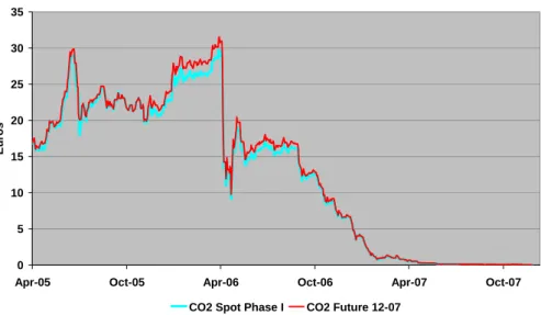
The evolution of Phase I EUA prices is shown in Figure 1. Phase I EUAs started to be traded around 17 euros and quite rapidly reached a first peak of 30 euros. Then, they were traded between 20 and 25 euros until mid April 2006, when they reached the second peak of 30 euros. With the publication of the information concerning the real

2 _{See Keppler (2009, forthcoming) for an exposition of both theories.}

3_{For more information on markets volumes and contracts see Mansanet-Bataller and Pardo (2008).} 4_{The prices on EUA futures and spot have been obtained from the web pages of the corresponding}

(6)

2005 emissions in April 2006, the EUA prices dropped to less than 15 euros in a few days. They continued to be traded around the 15 euros until September 2006 where they started the fall, finishing the trading period close to zero.

Figure 1: Spot and Futures Prices during Phase I

0 5 10 15 20 25 30 35

Apr-05 Oct-05 Apr-06 Oct-06 Apr-07 Oct-07

Eu

ro

s

CO2 Spot Phase I CO2 Future 12-07

Source: EEX and ECX web pages.

In what concerns the EUA data for the first year of Phase II we considered the spot prices from BlueNext as it has become the most important spot market in terms of volume, and ECX futures prices with delivery December 2009.5

2.2. Energy Variables

We considered the most representative prices for natural gas, coal and electricity in Europe. Concerning the futures prices on natural gas, we used the front contract price series of the Intercontinental Exchange Futures (ICE Futures). The Coal forward prices considered are the API 2 index published by McCloskey, which is one of the reference prices of coal in Europe.6_{Note that in order to perform our study, both data}

on gas and coal were converted into euros. All those data are obtained from the Reuters database.

In what concerns electricity prices, we took into account both spot and futures electricity prices from the French market Powernext. In both cases we used peak and base load electricity prices.7_{The futures prices used for Phase I are the 2007 calendar}

contract (electricity provision over one calendar year, in this case 2007) while the futures electricity prices for the first year of EU ETS Phase II are the 2009 calendar ones.8

5_{This data has been obtained from the market web pages: www.bluenext.fr. For more information on} market volumes, see Mansanet-Bataller and Pardo (2008).

6_{Specifically, those coal prices are CIF (Cost, Insurance and Freight) with delivery in ARA} (Amsterdam, Rotterdam and Antwerp).

7_{Those prices have been obtained from powernext web page:}_{www.powernext.fr}_. 8_{Note that finally, trading for the 2007 calendar ends naturally on 31}st_{December 2006.}

(7)

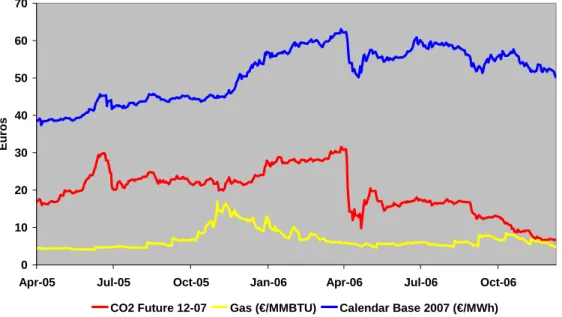
Figure 2 shows the evolution of natural gas, CO2 and electricity futures prices in the

Phase I of the EU ETS.

Figure 2: Evolution of natural gas, CO2 and electricity futures prices in Phase I

0 10 20 30 40 50 60 70

Apr-05 Jul-05 Oct-05 Jan-06 Apr-06 Jul-06 Oct-06

Eur

o

s

CO2 Future 12-07 Gas (€/MMBTU) Calendar Base 2007 (€/MWh)

Source: Reuters, Powernext and ECX web pages.

We also used in this study data on the Clean Dark Spread (CDS) and the Clean Spark Spread (CSS) provided by Tendances Carbone.9_{The CDS is calculated as the}

electricity cost minus the addition of carbon and coal costs. The CSS is similarly obtained as the electricity cost minus the addition of carbon and natural gas costs.

2.3. Stock Market Data

Finally, we considered the Eurostoxx 600 as a proxy of the expectations of general future economic activity.10_{In an efficient market, stock-prices are equal to the}

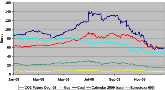
expected discounted flow of future dividends. Future dividends, however, depend on future profits and revenues which both depend heavily on general economic activity. Broad-based stock market indices such as the Eurostoxx 600 will smooth out any firm- or sector-specific differences in growth prospects. Such stock market indices are thus very good indicators of the expectations of general future economic activity. In order to have an idea of the evolution of all the variables considered in the study, we present in Figure 3 the evolution of CO2 spot and futures prices for the first year

of Phase II (2008) jointly with the energy price and the stock market evolution.

9_{For more information on the Tendances Carbone publication visit the Caisse des Dépôts website at} http://www.caissedesdepots.fr/spip.php?article647

10_{We thank Claude Mougiama and François Laguilliez of NYSE Euronext for making the 2005 – 2008} series of daily prices of the Eurostoxx 600 available to us.

(8)

Figure 3: Energy Prices and the Stock Market during Phase II 0 20 40 60 80 100 120 140 160

Jan-08 Mar-08 May-08 Jul-08 Sep-08 Nov-08

Eur

o

s

CO2 Future Dec. 09 Gas Coal Calendar 2009 base Eurostoxx 600

Source: Powernext and ECX web pages, NYSE Euronext and Reuters. Note that the units are euros per tonne, MWh or MMBTU, Stoxx rebased Index number.

2.4. Weather Variables

We considered the European temperature index published by Tendances Carbone. This index is a population weighted average on the temperatures of Spain, France, Germany and the United Kingdom.

From this index we obtained the “Unexpected temperature changes index” which tracks the spread between the index of European temperatures explained above and the average temperature on the same month during the past 10 years.

Finally, in order to not distinguish the sign of temperature differences (hotter or colder than in previous years), we have also considered both indexes in absolute terms. We named this index the “Absolute temperature changes index”.

2.5. Granger Causality Test Methodology

In order to establish a hierarchy of direct and indirect influences between different price series we used the Granger causality test (GCT). The Granger causality test looks at causality in the sense of precedence between the time series of two stationary variables. It is named after the first causality tests performed by Clive Granger (1969). It analyses the extent to which the past variations of one variable explain (or precede) subsequent variations of the other. Granger causality tests habitually come in pairs, testing whether variable xt Granger-causes variable yt and vice versa. All

permutations are possible: univariate Granger causality from xt to yt or from yt to xt,

(9)

In all cases, the different series need to be rendered stationary since applying Granger causality tests to non-stationary data can lead to spurious causality relationships.11

After applying standard stationary test such the Augmented Dickey Fuller unit-root test, all time series during the period between January 2005 and December 2007 proved to be non-stationary. Consequently, they were rendered stationary by taking first order differences. All Granger causality tests were thus performed with differenced data, which makes meaningful results harder to achieve. The fact that many results presented themselves in a very clear-cut manner underlines the pertinence of the results.

Nevertheless, even well-established Granger causality does not imply ‘causality’ in the colloquial sense of an unavoidable logical link but in the sense of inter-temporal precedence. Formally, the Granger causality test analyses whether the unrestricted equation

yt = α0 + ΣTi=1 α1i yt-i + ΣTj=1 α2j xt-j + εt with 0 ≤ i, j ≤ T

yields better results than the restricted equation

yt = β0 + ΣTi=1 β1i yt-i + εt with ΣTj=1 α2j xt-j = 0 (the null-hypothesis).

In other words, if H0, in which α21 = α22 =…= α2T = 0, is rejected then one can state

‘variable xt Granger-causes variable yt’.

Results of Granger causality tests are sensitive to the number of lags specified. In principle, one should include the maximum number of lags over which an economically meaningful relationship between two variables may exist. In this work, we consistently chose the lag that gave the most significant results.12

The result of the Granger causality test displayed will decide the choice of dependent and independent variable. Determining the direction of causality between the different price series will allow formulating the equation for the OLS estimation of the quantitative long-run relationship. Note that when performing the regression we use the Newey-West method in order to obtain consistent estimated of the variance of the parameters.

11 _{An earlier version of this presentation of Granger causality tests is contained in Keppler (2007).} 12_{The program used in this exercise, E-views, always tests for the null-hypothesis that variable X does}

not Granger-cause variable Y. E-views will thus calculate the F-statistic of the regression under the

null hypothesis that α21 = α22 =…= α2j = 0 and provides the probability that the null hypothesis is accepted. For probability values lower than 0.05 (5 per cent), we consider the Null hypothesis rejected and hence consider that variable X does Granger cause variable Y.

(10)

3. Causalities between CO

2

, electricity and gas prices during Phase I:

Empirical Results

3.1. Causality between CO2 Spot and Futures Prices

The first causality test we performed tested the link between CO2 futures prices to

CO2 spot prices. In concordance with earlier tests with slightly different time series

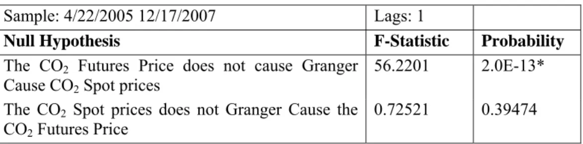
(see Keppler (2009, forthcoming), the causal relationship runs from the futures market to the spot market. The impact is immediate and very clear (the probability for futures prices not causing spot prices is essentially zero). This result is not unexpected given that the futures market was several times larger than the spot market: during Phase I, 65,754 kilotonnes were traded in BlueNext while 244,335 kilotonnes were traded in ECX. In the larger market the infrastructure for information gathering and research is more efficient and new information is thus integrated faster into the price.

Table 1: Causality tests results between CO2 Spot and Futures prices Sample: 4/22/2005 12/17/2007 Lags: 1

Null Hypothesis F-Statistic Probability

The CO2 Futures Price does not cause Granger

Cause CO2 Spot prices

56.2201 2.0E-13* The CO2 Spot prices does not Granger Cause the

CO2 Futures Price

0.72521 0.39474

Note: * denotes statistically significance at 1% level.

With a very strong one-way causality link, CO2 spot and futures prices evolve closely

linked together. The correlation coefficient for the two price series is a staggering 0.999157.13_{This is because an EUA is an easily storable financial instrument whose}

value at time t0 should not be fundamentally different from its value at time t1. Two

caveats apply, however:

1. Allowances must be traded in the same accounting period as the one in which they were allocated (i.e., Phase I or II respectively), and

2. The cost of carry, the cost of interest foregone by holding an EUA, must be compensated and prices for future delivery must be slightly above the spot price.

3.2. The Determinants of the CO2 Futures Price

The first question at this point is, of course, what determines the development of CO2

futures prices. The answer is not straightforward. First, meaningful statistical relationships are only discernible in Phase I between April 2005, when the ECX futures market opened, and April 2006, when the Commission’s announcement of member countries’ compliance set the market into a tailspin and supplanted economic reasoning with more event-driven political reasoning in the market. Second, during

(11)

the first year of Phase II, several relationships are discernible that point towards an interesting interaction of several factors.

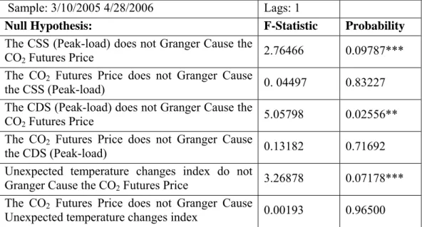
As we can appreciated in Table 2, CO2 futures prices are Granger-caused by the CSS

for peak-load electricity, the CDS for peak-load electricity as well as by the unexpected short-run changes in the “Unexpected temperature changes index” i.e. the European index corrected by the average temperature of the last 10 years.

Table 2: Causality tests results between CO2, CSS, CDS and unexpected

temperature differences

Sample: 3/10/2005 4/28/2006 Lags: 1

Null Hypothesis: F-Statistic Probability

The CSS (Peak-load) does not Granger Cause the

CO2 Futures Price 2.76466 0.09787***

The CO2 Futures Price does not Granger Cause

the CSS (Peak-load) 0. 04497 0.83227 The CDS (Peak-load) does not Granger Cause the

CO2 Futures Price 5.05798 0.02556**

the CDS (Peak-load) 0.13182 0.71692

Unexpected temperature changes index do not

Granger Cause the CO2 Futures Price 3.26878 0.07178***

Unexpected temperature changes index 0.00193 0.96500

Note: ** (***) denotes statistically significance at 5% (10%) level.

The CSS (Peak-load) is the difference between the price of peak-time electricity minus the variable costs of a gas-fired power plant (fuel costs plus carbon costs) per MWh. The CDS (Peak-load) is the difference between the price of peak-time electricity minus the variable costs of a coal-fired power plant (fuel costs plus carbon costs) per MWh. In essence, the above results mean that carbon prices rise when operators profits are large, which gives some credence to the rent capture hypothesis alluded to above. This hypothesis is further supported by the fact that the identified link is much stronger for CSS and CDS in peak-load when operators do have some market power rather than in base-load when market power is essentially absent. The index of “Unexpected temperature changes” is composed of a composite indicator, which measures on a day-by-day basis the divergence of the European temperatures index from the average of the index values in the ten preceding years. The result of the Granger Causality Test indicates rather intuitively that such differences had an impact on the price of a CO2 allowance for December 2007

delivery.

There were no other identifiable direct influences on the CO2 futures price such as

(12)

3.3. Determinants of Peak-load Clean Spark Spread (CSS) and Clean Dark Spread (CDS)

The causal influence on peak-load spreads, in particular the CDS, is also rather intuitive and fall into three distinct categories:

1. The influence of electricity spot prices;

2. The influence of the prices of the underlying fuels, i.e. gas and coal, and 3. The influence of temperatures (transmitted by electricity prices).

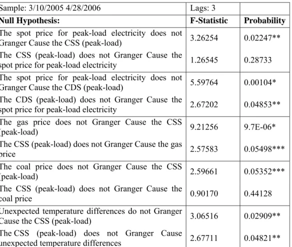
It is notable, as we can appreciate in Table 3, that all these relationships display their greatest strength with a three-day lag (relationships after shorter lags stay relevant, however). It is as if the different influences, notably the interaction between electricity spot prices and the gas price, needed some time to fall into place.

Table 3: Causality tests results between electricity, CSS, CDS, gas, coal and unexpected temperature differences

Sample: 3/10/2005 4/28/2006 Lags: 3

The spot price for peak-load electricity does not

Granger Cause the CSS (peak-load) 3.26254 0.02247** The CSS (peak-load) does not Granger Cause the

spot price for peak-load electricity 1.26545 0.28733 The spot price for peak-load electricity does not

Granger Cause the CDS (peak-load) 5.59764 0.00104* The CDS (peak-load) does not Granger Cause the

spot price for peak-load electricity 2.67202 0.04853** The gas price does not Granger Cause the CSS

(peak-load) 9.21256 9.7E-06*

The CSS (peak-load) does not Granger Cause the gas

price 2.57583 0.05498***

The coal price does not Granger Cause the CSS

(peak-load) 2.59661 0.05352***

The CSS (peak-load) does not Granger Cause the

coal price 0.90170 0.44128

Unexpected temperature differences do not Granger

Cause the CSS (peak-load) 3.06516 0.02909** The CSS (peak-load) does not Granger Cause

unexpected temperature differences 2.67711 0.04821**

Note: *(**,***) denotes statistically significance at 1% (5%,10%) level.

Two observations are noteworthy in this context. First, there is a very strong link between the gas price and the CSS for peak-load electricity which is due to the close link that gas prices have with electricity spot prices for peak-load (due to the fact that gas is the marginal fuel, which sets the electricity price). Second, the bi-directional causality between unexpected temperature differences and the CSS is not too

(13)

surprising. Market participants may react to recently announced weather changes or changes in the forecast. It is thus not unusual to find causality from financial variables to recorded weather data, which indicates precisely that the market reacts to weather forecasts.

3.4. What Drives Gas and Coal and Electricity Spot Prices?

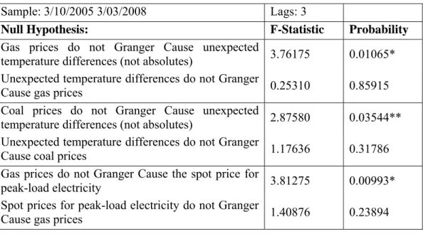
Pursuing this causal chain further, the results are again straightforward. The relationships for coal, gas and electricity prices are also stable over the whole three-year period of Phase I of the EU ETS.14_{As shown in Table 4, both gas and coal}

prices clearly react to forecasts of European temperatures. The reaction of the gas price is stronger given that it is determined in a European market, whereas coal is traded on an integrated global market. One also needs to mention that the reaction for gas and, in particular, coal prices is stronger for “non-absolute” temperature differences. This means that it does matter for gas and coal prices whether temperatures diverge upwards or downwards from the average of the previous ten years. This is not the case for the relationship between temperature and electricity prices or the CDS and the CSS which react mainly to absolute differences. This highlights the fact that gas and coal are not only inputs to power generation (which is equally used for air conditioning and heating) but also heating fuels in their own right. Warmer than expected days will make their price go down, colder than expected days will make their price go up.

Table 4: Causality tests results between gas, unexpected temperature differences, and coal

Sample: 3/10/2005 3/03/2008 Lags: 3

Gas prices do not Granger Cause unexpected

temperature differences (not absolutes) 3.76175 0.01065* Unexpected temperature differences do not Granger

Cause gas prices 0.25310 0.85915

Coal prices do not Granger Cause unexpected

temperature differences (not absolutes) 2.87580 0.03544** Unexpected temperature differences do not Granger

Cause coal prices 1.17636 0.31786

Gas prices do not Granger Cause the spot price for

peak-load electricity 3.81275 0.00993*

Spot prices for peak-load electricity do not Granger

14_{This is an indication that energy markets are more mature than the CO}

2 market, which is still finding its true underlying determinants among event-driven political interference. Another sign for differences in maturity is also that gas and coal markets move proactively on temperature forecasts, whether carbon markets react passively to recorded temperatures. This, however, this does not diminish the importance of the CO2 market and in particular the CO2 future market for influencing prices in other markets, most notably the market for electricity sold in the future market (see section 3.5).

(14)

Gas prices do not Granger Cause the spot price for

base-load electricity 2.12402 0.09579***

Spot prices for base-load electricity do not Granger

Note: *(**,***) denotes statistically significance at 1% (5%, 10%) level.

A second observation is that the gas price is an important driver for electricity spot prices. We have already mentioned the role of gas as the price-setting fuel in times of peak demand. The robust relationship between gas prices and prices for spot peak-load electricity, which becomes stronger, the greater the number of lags under consideration, is thus not surprising. The relationship with the spot price for base-load electricity is indeed a number of magnitude smaller, but still hints at the fact that gas is increasingly used also in base-load power production, most notably in Spain and the United Kingdom.

One additional fact merits brief discussion. If gas prices Granger-cause electricity spot prices and electricity spot prices through the CDS and the CSS influence the CO2

futures price, why does the gas price not show up directly in the CO2 futures price?

The reason is that gas prices are not the only influence of the electricity spot price. Electricity spot prices are also heavily influenced by the scarcity of capacity in the market, outages, stoppages etc., influences for which we are not testing directly in the present exercise (except indirectly through the electricity spot price, see 3.6 below). The CSS and the CDS that Granger-cause the CO2 futures price are thus the result of

the interplay between the gas price and the demand and supply balance in the electricity spot market and not of any single influence alone.

3.5. The Impact of CO2 Futures Prices on Electricity Futures Prices and the Stock

Market

It is time now to look into the other direction and to see which impact CO2 futures

prices have on other variables and, in particular, electricity futures and spot prices. This after all is the central hypothesis ruling the functioning of the carbon price – electricity price relationship. We have already seen that things are not so straightforward in the short run when the CSS and the CDS (and with them the spot prices for electricity peak-load) have an impact on CO2 futures prices. However, as

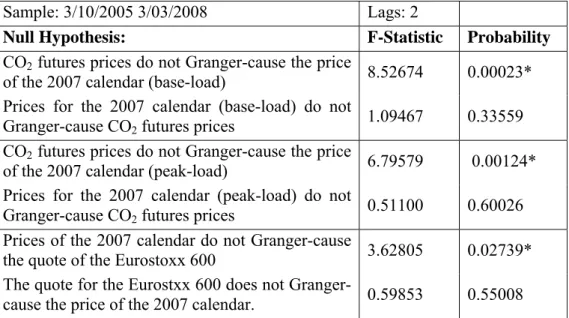
we can appreciate in Table 5, in the long run the postulated standard relationship still holds and there is a clear link from CO2 futures price for delivery in December 2007

and the 2007 calendar. In addition, there is a somewhat unexpected but statistically stable relationship between the price of long-term forward delivery of electricity and a broad-based index of European companies, the Eurostoxx 600.

Let us take the two arguments step-by-step. The impact of CO2 futures prices on

electricity futures prices (the 2007 calendar in our case) is abundantly clear and is confirmed over the whole three-period as well as over any number of lags (it actually increases with a greater number of lags). This means that the CO2 price is today part

(15)

and parcel of the long-term cost of generating electricity. The relationship holds for both base-load and peak-load but is stronger for base-load as it should be the case since coal (heavily used in base-load power production) is more carbon-intensive and hence more dependent on the carbon price than gas (heavily used in peak-load power production).

Table 5: Causality tests results between CO2 and electricity futures prices and

the stock market

Sample: 3/10/2005 3/03/2008 Lags: 2

CO2 futures prices do not Granger-cause the price

of the 2007 calendar (base-load) 8.52674 0.00023* Prices for the 2007 calendar (base-load) do not

Granger-cause CO2 futures prices 1.09467 0.33559

CO2 futures prices do not Granger-cause the price

of the 2007 calendar (peak-load) 6.79579 0.00124* Prices for the 2007 calendar (peak-load) do not

Granger-cause CO2 futures prices 0.51100 0.60026

Prices of the 2007 calendar do not Granger-cause

the quote of the Eurostoxx 600 3.62805 0.02739* The quote for the Eurostxx 600 does not

Granger-cause the price of the 2007 calendar. 0.59853 0.55008

Our final result is somewhat of a curiosity but the results hold well over the 2005 and 2006 at any number of lags: the price of the 2007 calendar Granger-causes the quote of the Eurostoxx 600 a broad-based benchmark index for European shares. The result if verified by further research would, of course, be of momentous interest: carbon prices drive electricity prices which drive economic activity. So far, so good, the relationship between the two variables is positive, however. This points probably to a spurious causality relationship where general economic growth drives both electricity prices and demand as well as stock market returns, even though the test used stationary data (first differences) and the Durbin-Watson statistic of a simple regression is close to 2. At the very least, the finding is interesting enough to warrant further study.

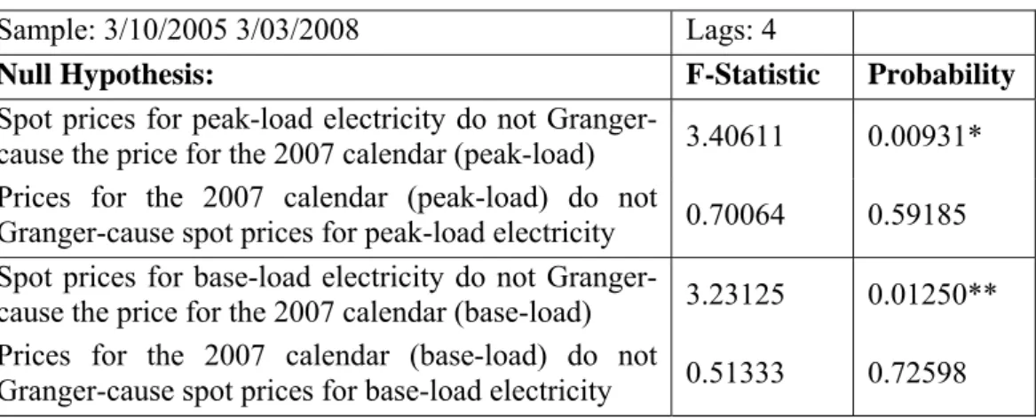
3.6. Electricity Futures Prices as the Result of Gas and Electricity Spot Prices

There is an additional impact on electricity futures prices, which are electricity spot prices. This is due to the fact that electricity spot prices, especially peak spot prices indicate scarcity in the market and thus provide information about available capacity. The impact is immediate but strongest after four days.

(16)

In other words, while CO2 futures prices are an important determinant of electricity

futures prices, they are not the only determinant. The two types of information conveyed by the two sets of data are of different nature. The price of CO2 futures

regards variable costs. The information conveyed by electricity spot prices regards the availability of sufficient capacity in the market. Both, CO2 futures and electricity spot

prices, however, also partially contain information about gas prices, which thus also becomes an important (indirect, mitigated and transformed) input into long-term electricity futures prices. The results are shown in Table 6.

Table 6: Causality tests results between electricity spot and futures prices

Sample: 3/10/2005 3/03/2008 Lags: 4

Spot prices for peak-load electricity do not

Granger-cause the price for the 2007 calendar (peak-load) 3.40611 0.00931* Prices for the 2007 calendar (peak-load) do not

Granger-cause spot prices for peak-load electricity 0.70064 0.59185 Spot prices for base-load electricity do not

Granger-cause the price for the 2007 calendar (base-load) 3.23125 0.01250** Prices for the 2007 calendar (base-load) do not

Granger-cause spot prices for base-load electricity 0.51333 0.72598

Note: *(**) denotes statistically significance at 1% (5%) level.

3.7. Putting it All Together

The different causality relationships identified on the preceding pages gives rise to a rather complicated interplay of different energy markets during Phase I of the EU ETS, which nevertheless allows a coherent picture that is perfectly consistent with standard theoretical or practical considerations.

Figure 4: Causality relationships identified for Phase I of the EU ETS

CO2 Spot Coal

Weather CSS & CDS CO2 Future Electricity Future Stoxx Gas

(Scarcity) Electricity Spot

The most important observation is undoubtedly that carbon prices, in particular CO2

futures prices, have firmly established themselves at the heart of the interplay of European electricity markets. They depend during Phase I primarily on the profit margins in the electricity sector as well on short term weather changes.

(17)

Several additional points are noteworthy:

1. Spot and futures markets are linked across commodities;

a. there exist, for instance, no important relationships between spot market variables only;

b. electricity spot markets convey important information about scarcity of capacity to futures market

2. Weather (temperature) changes are an important driver for short term price changes in almost all markets;

3. Gas markets are more integrated with electricity markets than coal markets given that the price on the latter is determined globally.

3.8. Quantitative Testing with OLS

The previous causality analysis allows us to determine the dependent and the independent variables for the regression in order to formulation an equation for further econometric testing of the quantitative strength of the relationships. The results of the previous sections leave no doubt that during Phase I of the EU ETS the price for the annual electricity futures contract with delivery 2007 (calendar 2007) depends on the price of CO2 futures for 2007 delivery. That means that we may be

able to explain those electricity prices using the information on the other variables considered such as the price of CO2, the gas prices and the CSS. The full model is

specified as follows: t t gas t CO t feleb r diff CSS r r , =α + 2, +log ( )+ ,₋₁+ε

Where r_feleb,_t are the returns of electricity futures prices with delivery 2007 at

time t, α is a constant, r_CO2,_t are the returns of CO2 with delivery December

2007 at time t, logdiff(CSS) are the log-differentiated series of CSS, r_gas_,_t₋₁ are

the returns of gas month-ahead contract in t-1, and is the error term.

The results of the regression are shown in Table 7. Note that we used the adjusted sample from 7 April 2005 to the 28 April 2006 in order to only consider the prices before the CO2 crash provoked by the surplus of allowances distributed for Phase I.

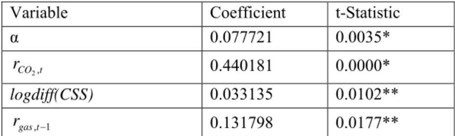
Table 7: OLS results for Phase I of the EU ETS

Variable Coefficient t-Statistic

α 0.077721 0.0035* t CO r 2, 0.440181 0.0000* logdiff(CSS) 0.033135 0.0102** 1 ,t− gas r 0.131798 0.0177**

(18)

R-squared 0.391168 Mean dependent var. 0.050047 Adjusted R-squared 0.382429 S.D. dependent var. 0.634682 S.E. of regression 0.498769 Akaike info criterion 1.465255 Sum squared resid. 51.99311 Schwarz criterion 1.528378 Log likelihood -152.0496 F-statistic 44.76004 Durbin-Watson stat 2.376293 Prob(F-statistic) 0.000000

The coefficients of all those variables are statistically significant at 5% level and two of them (the coefficient for the CO2 returns and the CSS base) are statistically

significant at 1% level. That is, the electricity prices for delivery 2007 depend on CO2

returns, gas returns, and the CSS. With these elements we explain the cost of electricity by two important factors: (i) the price of gas, and (ii) the monopoly power (which is reflected by the CSS).

In order to measure the goodness of the regression we focus on the R-squared and the Adjusted R-squared which are equal to 0.391168 and 0.382429, respectively. This regression confirms the results of the previous sections and explains satisfactorily the electricity price formation.

4. Causalities between CO

2

, electricity and gas prices during Phase II:

Empirical Results

Phase I was a period of intense learning for all market participants. During 2008, the first year of Phase II of the EU ETS, observers and market participants thus had good reason to expect a maturing of the European carbon market and the emergence of more stable relationships between different variables. In addition, there was hope that the emerging relationships would correspond to economic theory as well as to the observable facts of industrial reality.

As we have seen, this was only very partially the case during Phase I. While the impact of CO2 futures prices to electricity futures prices was statistically undeniable

and clearly corresponded to the expectations of market participants, there was little industrial reason that a system with an over-allocation of allowances should produce average prices of € 12 for an EUA to be fed through to electricity prices.

The interest of this chapter is to test what happened during the first year of Phase II of the EU ETS. We may already say that the stability of the CO2 futures contract for

December 2009 delivery throughout the descent of the price of the Phase I allowance to zero as well as the beginning of Phase II seemed to indicate that the hopes that the emerging relationships would correspond to economic theory as well as to the observable facts of industrial reality were well founded for the Phase II of EU ETS. Then came the crisis… With the Eurostoxx 600 stock-market index loosing more than 50% from its high in June 2007 and almost 45% from 1 January 2008 until 31 December 2008, it is clear that 2008 was no ordinary year. If stock prices are indeed a forward-looking indicator of future profits and economic growth, it is obvious that

(19)

economic growth, and with it industrial output and the demand for carbon allowances, would be less than originally envisioned. Obviously, this played an important role in the decline from € 24 to € 16 of the December 2009 contract during the year 2008 and this section will look closely at the different causal relationships that are active in this decline.

4.1. Causality between CO2 Spot and Futures Prices

One relationship that remained stable between Phase I and the first year of Phase II is the relationship between CO2 spot and futures prices. CO2 futures prices continue

drive CO2 spot price. However, as we can appreciate in Table 8 the relationship is

becoming slightly less mechanical than in the past. The probabilities for Granger causality running from futures prices to spot prices have weakened and the probabilities for the reverse relationship have strengthened. CO2 spot prices are

slightly more autonomous today than during Phase I. This may be a reflection of the growing importance of the spot market both in absolute and in relative terms. During 2008, 250 million tonnes of CO2 were traded on the Bluenext spot market, while

1,998 million tonnes were traded on the ECX futures market. In 2006, the figures had been 31 million and 452 million tonnes of CO2 respectively.

Table 8: Causality test results between CO2 spot and futures prices Sample: 1/02/2008 12/31/2008 Lags: 1

CO2 futures prices do not Granger-cause CO2 spot

prices 5.54789 0.01941**

CO2 spot prices do not Granger-cause CO2 futures

prices 1.61299 0.20546

Note: ** denotes statistically significance at 5% level.

4.2. The Determinants of the CO2 and the Electricity Futures Price

Looking at the drivers of the CO2 futures price, one of the key relationship of Phase I

is confirmed. Also in Phase II, CO2 futures prices are Granger-caused by the spreads

between operating costs (fuel costs plus CO2 costs) and the electricity price. The

Table 9 shows that significant causal relationships exist between all four possible spreads (if we consider peak and base electricity prices) and the CO2 futures price.

The relationships are all immediate and are confirmed over a higher number of lags.

Table 9: Causality test results between CO2 futures prices, CDS, and CSS Sample: 1/02/2008 12/31/2008 Lags: 1

The CDS base-load does not Granger-cause CO2

futures prices 7.51611 0.00655*

CO2 futures prices does not Granger-cause the CDS

(20)

The CDS peak-load does not Granger-cause CO2

futures prices 6.16731 0.01366**

CO2 futures prices does not Granger-cause CDS

peak-load 5.34612 0.02157**

CSS base-load does not Granger-cause CO2 futures

prices 4.58878 0.03314**

CO2 futures prices does not Granger-cause CSS

base-load 3.18497 0.07552***

CSS peak-load does not Granger-cause CO2 futures

prices 4.51401 0.03459**

CO2 futures prices does not Granger-cause CSS

peak-load 3.34979 0.06839***

Note: *(**,***) denotes statistically significance at 1% (5%, 10%) level.

As already mentioned in previous sections, this Granger causality relationship from the CDS and CSS towards CO2 futures prices provides some indication for the

hypothesis that carbon prices (in the absence of sufficient abatement activity to establish a cost-based carbon price) are determined at least partly by the ability of electricity producers to extract rents from the scarcity of available capacity. The evidence for this sort of link is even stronger, as shown in Table 10, during the first year of Phase II than during Phase I due to the fact that for a number of lags greater than three (four and higher) electricity futures prices are becoming an important determinant for CO2 futures prices. It is important to underline here that, as we have

seen, during Phase I this particular causality relationship was still running from CO2

futures prices to electricity futures prices.

Table 10: Causality test results between CO2 and electricity futures prices Sample: 1/02/2008 12/31/2008 Lags: 4

Prices for the 2009 calendar base-load does not

Granger-cause CO2 futures prices 3.53933 0.00790*

CO2 futures prices does not Granger-cause prices

for the 2009 calendar base-load 1.02354 0.39572

As we will see, the relationship running from futures prices for base-load electricity to CO2 is not only very stable but also very important, since it feeds through a number

of additional causality relationships. In other words, any effect Granger-caused by CO2 futures prices exhibits an even stronger dependence on electricity futures prices.

Conversely, the effects of the CSS and CDS on electricity futures prices are even stronger than their effects on CO2 futures prices.

(21)

4.3. Influences of the CO2 and the Electricity Futures Price

Before coming to the role of electricity futures prices, it is useful to look briefly at the impacts of the CO2 futures price, mindful of the fact that these impacts probably

originate with electricity futures prices and that CO2 futures prices serve only to “pass

through” these impacts.

However, whether one considers CO2 or electricity futures prices, it is surprising to

see that their impact extends mainly to the prices of fuels, that is, coal and, to a lesser extent, gas. Conventional wisdom would, of course, expect causality to run into the other direction. Either these fuels used as inputs into power production would cause the price of electricity, or the prices of these fuels would eventually determine opportunities for fuel switching and thus have an impact on the price of carbon allowances.

Well, the statistical connection, as shown in Table 11 and Table 12, clearly goes primarily into the other direction (strictly speaking the link between coal and CO2

futures prices is bi-directional, with a link from CO2 to coal being several orders of

magnitude more likely). We may see in Table 11 that the link with coal prices is clear, immediate and stable over any number of lags.

Table 11: Causality test results between CO2 futures prices and coal Sample: 1/02/2008 12/31/2008 Lags: 1

Null Hypothesis: F-Statistic Probability

Coal price does not Granger-cause CO2 futures prices 4.28800 0.03940**

CO2 futures prices does not Granger-cause Coal price 21.8897 4.7E-06* Note: *(**) denotes statistically significance at 1% (5%) level.

The second link with gas, as indicated in Table 12, is considerably weaker and only kicks in after seven lags, but from then on it is also stable.

Table 12: Causality test results between CO2 futures prices and natural gas Sample: 1/02/2008 12/31/2008 Lags: 7

CO2 futures prices does not Granger-cause Gas price 1.86211 0.07662***

Gas does not Granger-cause CO2 futures prices 1.26283 0.26964 Note: *** denotes statistically significance at 10% level.

The most likely explanation is that electricity and carbon futures markets process relevant information, notably on future demand, quicker than the coal spot or the market for the one-month gas forward contract market. Once more, this shows that the notion of “causality” in the term “Granger causality” needs to be treated with circumspection. Concerning gas prices it also needs to be considered that they were available only in the form of month-ahead prices. There is thus a case to be made for the fact that gas prices correspond to some sort of slower-moving average price which will only react to a certain amount of accumulated information.

(22)

In what concerns electricity, we already mentioned that the same relationships are obtained in an even more pronounced form for the electricity futures price. In particular, as shown in Table 13, the link with the coal spot price is very strong, immediate and stable over any number of lags.

Table 13: Causality test results between electricity futures prices and coal

Sample: 1/02/2008 12/31/2008 Lags: 1

Granger-cause Coal prices 69.5097 4.9E-15* Coal prices does not Granger-cause prices for the

2009 calendar base-load 1.94771 0.16406

The link with the gas price is again much more tenuous with a probability for the absence of any link being 7.328 per cent and only comes in after a one-week delay. Concerning the coal price, however, there exists another interesting Granger causality relationship, which is perfectly coherent with theory and intuition, but which alas gives little clue to the connections between carbon and electricity prices. This relationship regards the significant impact the stock market has on the coal price. This is perfectly plausible given that the stock market is a good indicator of economic growth and given the strong interconnection of stock markets all over the world for global growth. That European coal prices should be determined by global growth in addition to the outlook for European electricity demand makes perfect sense. The causality results are shown in Table 14.

Table 14: Causality test results between Eurostoxx 600 and coal

Sample: 1/02/2008 12/31/2008 Lags: 1

Euro Stoxx 600 does not Granger-cause Coal prices 6.47081 0.01156** Coal prices does not Granger-cause Euro Stoxx 600 0.88561 0.34757

Beyond this interesting link to the coal market, the Eurostoxx 600 does not maintain any further statistically verifiable links with the variables tested for in this analysis. Nevertheless, there is little doubt that the incipient financial and economic crisis is responsible for much of the decline.

4.4. Determinants of Electricity Futures Prices

The futures prices for base-load electricity that have such an important influence on the CO2 futures price are also determined, as we can appreciate in Table 15 by the

CSS and the CDS. This holds both for the base-load as well as for the peak-load spreads with the strongest influence coming from the CDS base-load.

(23)

Table 15: Causality test results between electricity futures prices, CDS, and CSS

Sample: 1/02/2008 12/31/2008 Lags: 1

Granger Cause CDS base-load 5.63547 0.01835** CDS base-load does not Granger-cause prices for the

2009 calendar 11.4614 0.00082*

Prices for the 2009 calendar does not Granger-cause

CDS peak-load 4.25135 0.04024**

CDS peak-load does not Granger-cause prices for the

2009 calendar 10.9373 0.00108*

CSS base-load does not Granger-cause prices for the

2009 calendar 9.66787 0.00209*

CSS base-load 0.14963 0.69922

CSS peak-load does not Granger-cause prices for the

2009 calendar 10.1873 0.00159*

CSS peak-load 0.52866 0.46784

Again, the most likely explanation is that the current CSS and CDS indicate the profit potential in the electricity market and thus provide an indication about demand (in particular the inelasticity of demand) and thus about the value of future electricity production.

4.5. Further Determinants of Electricity Futures Prices (peak-load)

The causality relationships from the spreads, both CSS and CDS, towards electricity futures prices are even stronger for peak-load.

The probabilities for the absence of any link lie between 0.00007 and 0.0002 per cent. After three periods there is also Granger causality identifiable from electricity spot prices to electricity futures prices (see Table 16).

Table 16: Causality test results between electricity spot and futures prices

Sample: 1/02/2008 12/31/2008 Lags: 3

Electricity spot prices (peak-load) do not Granger

Cause electricity futures prices (peak-load) 2.54514 0.05667** Electricity futures prices (peak-load) do not

Granger Cause electricity spot prices (peak-load) 0.30421 0.82234

This link exists, however, only for the peak-load calendar, not for the base-load calendar, which in this context is the more interesting given that it Granger causes

(24)

CO2 futures prices. The link between futures peak-load electricity and spot prices

(peak-load) is again mediated by capacity available for electricity production. The electricity spot market is essentially a market for short-term adjustment. This means the level of peak-load prices indicates to which extent expensive marginal capacity had to be added to system. It thus provides information about available capacity or scarcity to the forward market.

In return, electricity spot prices (both base-load and peak-load) have strong Granger causality with changes in the deviation of European temperatures from their historical average, as we can appreciate in Table 17.

Table 17: Causality test results between temperatures and electricity spot prices

Sample: 1/02/2008 12/31/2008 Lags: 1

The log-differentiated index of “Unexpected

temperature changes” does not Granger-cause Spot

prices for peak-load electricity

5.79718 0.01677** Spot prices for peak-load electricity does not

Granger-cause the log-differentiated index of “Unexpected temperature changes”

0.34690 0.55640

This link is, of course, mediated by electricity demand, which rises to the extent that temperatures are different from expectations. As one would expect for the electricity market, it does not matter whether these deviation are reported as real or as absolute figures. This is due to the fact that higher than average temperatures will cause air conditioning to go up, while colder than average figures will cause electric heating to increase.

Considering the role of temperatures it is worthwhile to briefly consider gas prices which react only to real temperature differences as shown in Table 18. This makes again perfect sense. Absolute figure (indicating always positive deviations) would in fact be met by price movements up or down in the gas market. Gas prices would go up in colder weather and down in warmer weather. Temperature deviations in absolute terms will thus explain less about gas price movements than temperature deviations in real terms.

Table 18: Causality test results between temperatures and gas

Sample: 1/02/2008 12/31/2008 Lags: 1

Gas prices doe not Granger-cause unexpected

temperature changes 8.62911 0.00361**

Unexpected temperature changes do not

Granger-cause gas prices 2.01366 0.15712

(25)

In the gas market we also encounter the phenomenon already observed in Phase I that gas prices precede temperature changes rather than the other way round. This implies, of course, again that gas prices react to temperature forecasts rather than to observed temperatures. In fact, the causality link gets less pronounced beyond 5 days although it does not disappear altogether.

4.6. What Determines the Clean Spark Spread and Clean Dark Spread?

Given the role of the CSS and the CDS, the difference between variable costs including the cost of carbon permits and the electricity price, it is logical to ask which Granger causalities can be identified in their formation. The answer is very clear: the clean spreads for the first year of the Phase II of the EU ETS depend on the gas price. Probabilities for Granger causalities are immediate, strong (i.e., the probabilities for the absence of Granger causality are close to zero) and persist over several lags, as shown in Table 19. In particular the CDS base-load, important because it has the closest link with futures prices for base-load electricity, has very strong Granger causality coming from the gas price. As for the gas price, we have seen in the previous chapter that it reacts to changes in temperature.

Table 19: Causality test results between gas CDS, and CSS

Sample: 1/02/2008 12/31/2008 Lags: 1

Null Hypothesis: F-Statistic Probability

Gas prices do not Granger Cause the CDS base-load 31.4386 5.4E-08* The CDS base-load does not Granger Cause gas prices 1.81770 0.17879 Gas prices do not Granger Cause the CDS peak-load 31.1421 6.2E-08* The CDS peak-load does not Granger Cause gas prices 1.49293 0.22290 Gas prices do not Granger Cause the CSS base-load 5.59160 0.01880** The CSS base-load does not Granger Cause gas prices 0.40605 0.52456 Gas prices do not Granger Cause the CSS peak-load 12.9695 0.00038* The CSS peak-load does not Granger Cause gas prices 0.59940 0.43953

4.7. Putting it All Together

The results for the first year of Phase II of the EU ETS are, finally, not all that different to the results obtained for Phase I. Again, a central axis running from temperature changes over the gas price and the CDS and CSS to the carbon and electricity markets can be identified. Figure 5 summarizes those relationships.

(26)

Figure 5: Causality relationships identified for Phase II of the EU ETS

Eurostoxx Coal

Temperature Gas CDS, CSS Electricity Future CO2 Future CO2 Spot

(Peak-load only)

(Scarcity) Electricity Spot

There are, however, several differences. First and most importantly, the causality relationship between CO2 futures prices and electricity futures prices (base-load) is

now reversed, with the base-load calendar now at the heart of the interplay between carbon, electricity and gas markets. Second, coal prices are no longer a driver but a follower in this causal chain. While the result is statistically unassailable, it demands further testing in the future given its inconsistency with the fact that the coal market is, at least in principle, a global market driven by global developments. In the same vein sense, the third important difference with Phase I of the EU ETS is the role of the stock market as a driver rather than as a follower of events in energy markets, is rather convincing especially given recent macroeconomic events.

4.8. Quantitative Testing with OLS

As in the case of the analysis of the interplays between daily carbon, electricity and gas prices during the Phase I of the EU ETS, we use de results of the causality tests for the first year of Phase II of the EU ETS (2008) to determine the dependent and independents variables for the regression as well as the lag. In this case, the most reasonable choice is to consider CO2 futures prices for Phase II (December 2009

contract) as the dependent variable. The independent variables are the spot peak load electricity, the futures base load electricity, the CDS base, the unexpected temperature differences, the Eurostoxx 600 stock-market index, and natural gas prices. The model is specified as follows: t t Gas t stoxx t t t feleb t selep CO r r diff CDS temp r r r 2 =α+ ,₋2+ ,₋4 +log ( )₋1+ ₋3+ , + ,₋1+ε

Where r_CO2,_tare the CO2 returns of the futures contract traded at ECX with delivery December 2009 at time t, are the spot electricity peak returns at time t-2,

are the futures electricity base returns at time t-4, logdiff(CDS)

2 ,t− selep r 4 ,t− feleb

r t-1 are the

log-differentiated series of CDS base at time t-1, tempt-3 are the European index

temperatures differences with the European 10 years average (the “difference index”), are the Eurostoxx 600 returns at time t, and are the natural gas returns at time t-1. The results are shown in Table 20. Note that the sample period in this case runs from 8

t stoxx

r , rGas,t−1

(27)

Table 20: OLS results for Phase II of the EU ETS

Variable Coefficient Probability

α -0.010550 0.7392 2 ,t− selep r 0.003744 0.0625*** 4 ,t− feleb r 0.068922 0.0067* logdiff(CDS)t-1 0.025551 0.0067* tempt-3 -0.021741 0.0738*** t stoxx r , 0.029021 0.0000* 1 ,t− Gas r 0.203933 0.0893***

Note that * (***) means statistically significant at 1% (10%) level.

R-squared 0.196511 Mean dependent var. -0.032727 Adjusted R-squared 0.176914 S.D. dependent var. 0.519226 S.E. of regression 0.471063 Akaike info criterion 1.359627 Sum squared resid. 54.58742 Schwarz criterion 1.457389 Log likelihood -164.9928 F-statistic 10.02749 Durbin-Watson stat 1.732885 Prob(F-statistic) 0.000000

As we can appreciate, the coefficients of all those variables are statistically significant. The electricity futures contract, the CDS and the Eurostoxx 600, are statistically significant at 1% while the other variables are at 10%. Note that the R-squared of this regression is 0.196511 and the Adjusted R-R-squared is 0.176914. As shown by those results, the relationship among all those variables is more complex than during the Phase I of the EU ETS and they confirm the short-term rent capture theory implying a causal link from electricity to carbon prices. In this theory, electricity operators monetize their scarcity rents that show up in higher electricity prices in the form of the prices carbon permits, which constitute a fixed factor of production and thus earn “rent” in the classical sense of the term.15_{We may also}

underline that there is an important influence of the electricity returns and gas returns on CO2 futures returns. Note that the importance of the impact of Eurostoxx 600

returns may be explained by the decrease in the worldwide demand that affects all energy markets (CO2 and electricity included).

15_{See Keppler (2009, forthcoming) “The interaction between the EU ETS and European electricity} markets”, in Convery et al.

(28)

5. Summary and Concluding Remarks

In this article we analyzed the causalities among several energy related variables, CO2

and weather both for Phase I of the EU ETS and the first year of the Phase II of the EU ETS.

The main results obtained include that the two periods exhibit several structural similarities, such as the Granger causality from CO2 futures to CO2 spot prices or the

importance of spreads rather individual prices variables in the determination of the CO2 futures price.

However, one key change compared to Phase I, is that during Phase II the prices for electricity futures, and in particular the 2009 calendar, are at the centre of the web that the different commodity prices maintain with each other.

Additionally, somewhat surprisingly (but statistically unequivocally), gas and coal prices are at the end of the causal chain rather than at the beginning as intuition would suggest.16

Finally, note that with Phase I being a trial period characterized by massive over-allocation, and with the first year of Phase II (2008) being marked by a disruptive economic crisis, it will be interesting to continue the study of Granger causalities with data generated under “normal” micro- and macroeconomic conditions. Hopefully, this time will not be too far off in the future.

16

There is one – so far untested – hypothesis that might explain why gas and coal prices reacted only

with a lag to the changes in expectations that were underway. This hypothesis is that during the first nine months of 2008 operators were still acting on the assumption of “de-coupling”. In other words, market participants had different assumptions about European and global markets. In this assumption, electricity and carbon prices would fall due to lower economic growth in Europe but gas and coal prices would remain stable (or even continue to rise) due to continuing economic growth in Asia, Russia and the Middle East. Once the “de-coupling” hypothesis became untenable, also gas and coal prices joined the march southwards.

(29)

6. References

Alberola, E., Chevalier, J., and Chèze, B., 2008, “Price Drivers and Structural Breaks in European Carbon Prices 2005–2007”. Energy Policy, 36(2), 787-797.

Benz, E. and Trück, S., 2008, “Modeling the price dynamics of CO2 emission

allowances”, Energy Economics 31 (2009) 4–15.

Convery, F., de Perthuis, C. and Ellerman, A. D., 2009 (Forthcoming), The European

carbon market in action: lessons from the first trading period. Cambridge:

Cambridge University Press.

European Parliament, 2003, Directive 2003/87/EC of the European Parliament and of the Council of 13 October 2003. “Establishing a Scheme for Greenhouse Gas Emission Allowance Trading within the Community and Amending Council Directive 96/61/EC”. Official Journal of the European Union L275/32. 25th October 2003.

Granger, C., 1969, “Investigating Causal Relations by Econometric Models and Cross-Spectral Methods”, Econometrica 37, P. 424 – 438.

Keppler, J. H., Bourbonnais, R. and Girod, J., 2007, The Econometrics of Energy

Systems, Palgrave Macmillan, London, 350 p.

Keppler, J. H., 2009 (Forthcoming), “The interaction between the EU ETS and European electricity markets”, in Convery et al. (2009, forthcoming).

MacKinnon, J. G., 1991, “Critical Values for Cointegration Tests, Long-run economic relationships: Readings in cointegration”, Advanced Texts in Econometrics, Engle, RF.: Granger, C. W. J. (eds.), Oxford University Press, 267-276.

Mansanet-Bataller, M. and Pardo, A., 2008, “What You Should Know About Carbon Markets”, Energies 1, 120-153.

Mansanet-Bataller, M., Pardo, A. and Valor, E., 2007, “CO2 Prices, Energy and