Some elliptic problems with singularities
197
0
0
Texte intégral
Figure
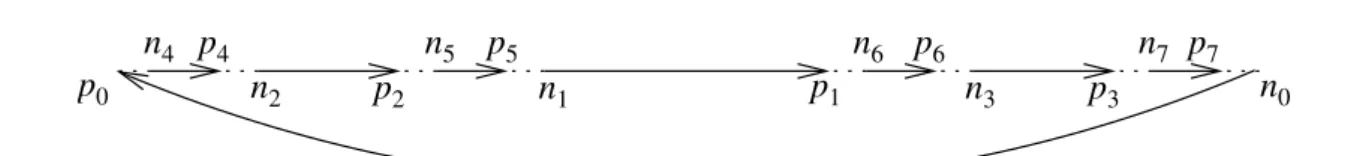
![Fig. 7.3 – A finite path Γ from q to r and the cycle [Λ] associated to Γ](https://thumb-eu.123doks.com/thumbv2/123doknet/2315009.27606/173.892.114.775.136.385/fig-finite-path-g-cycle-l-associated-g.webp)
+4


Documents relatifs