HAL Id: hal-01879566
https://hal.archives-ouvertes.fr/hal-01879566
Submitted on 24 Sep 2018
HAL is a multi-disciplinary open access
archive for the deposit and dissemination of sci-entific research documents, whether they are pub-lished or not. The documents may come from teaching and research institutions in France or abroad, or from public or private research centers.
L’archive ouverte pluridisciplinaire HAL, est destinée au dépôt et à la diffusion de documents scientifiques de niveau recherche, publiés ou non, émanant des établissements d’enseignement et de recherche français ou étrangers, des laboratoires publics ou privés.
Pseudo-dynamic simulation on a district energy system
made of coupling technologies
Getnet Tadesse Ayele, Mohamed Mabrouk, Pierrick Haurant, Björn Laumert,
Bruno Lacarrière
To cite this version:
Getnet Tadesse Ayele, Mohamed Mabrouk, Pierrick Haurant, Björn Laumert, Bruno Lacarrière. Pseudo-dynamic simulation on a district energy system made of coupling technologies. ECOS 2018 : 31st International Conference on Efficiency, Cost, Optimization, Simulation and Environmental Im-pact of Energy Systems, Jun 2018, Guimaraes, Portugal. �hal-01879566�
Pseudo-dynamic simulation on a district energy
system made of coupling technologies
Getnet Tadesse Ayelea,b, Mohamed Tahar Mabroukc, Pierrick Haurantd Björn
Laumerte and Bruno Lacarrièref
a,c,d,f IMT Atlantique, Department of Energy Systems and Environment, GEPEA, F-44307 Nantes, b,e Department of Energy Technology, KTH Royal Institute of Technology, 100 44 Stockholm, Sweden,
b[email protected] (CA) c[email protected] d[email protected] e[email protected] f[email protected] Abstract:
As part of an effort towards the future smart energy system, integration of different distributed generation technologies is proposed in literature. These technologies include heat pumps, gas boilers, combined heat and power (CHP) plants, solar photo-voltaic (PV) and so on. Some of these technologies couple different energy carriers in which case the independent analysis of each network could lead to unrealistic results. Optimization of heat pumps and CHP plants in coupled electricity and heating network, for example, needs consideration of both networks’ parameters in order to get results that are optimal in both networks. The first step in such optimization process is to have a load flow model (as an equality constraint) for the two coupled networks. Even though many researchers tried to address optimization of energy mixes at a district level, they did not consider the details of network parameters. And hence, too little has been done to investigate the effect of different distributed generation technologies on the operational parameters of different energy networks. This paper deals with a pseudo-dynamic simulation of a district energy system that consists of coupled electricity and heating networks. The details of transmission line and pipe parameters together with the coupling devices are modelled using an extended energy hub approach. A network of six energy hubs with different distributed generation technologies such as heat pump, gas boiler, CHP and Solar PV is considered in the simulation. Time series data for demands and generations at different hubs are used on hourly basis. The CHP and heat pumps are scheduled to operate in certain period of the year while the PV output follows the annual solar radiation. Annual pseudo-dynamic load flow simulation is done to see how the operational parameters and power losses in the network vary with hourly changes in demands, generations and loading of coupling technologies.
Keywords:
CHP, Coupled electricity and heating networks, Heat pump, Multi-carrier energy networks, Pseudo-dynamic simulation, Solar PV.
1. Introduction
District energy systems consists of different energy carriers such as heat, electricity, gas, water, hydrogen and others, which as a whole is referred to as multi-carrier energy system (MCES) [1]. As the demands are usually located at a different geographical place from the sources, MCES always consists of a network of pipes or transmission lines for each energy carrier to deliver power to the end users. Although the network for one energy carrier is independent from the other, there are coupling technologies at the source or at the end user that couple different energy carriers. For example, poly-generation technologies, such as CHP, produce both heat and electricity from different types of fuels (waste, biomass, gas etc.). As a result, they are used as links between electricity, heating and fuel networks. The coupling between different energy carriers gives additional alternatives to supply a given demand from different energy carriers. Such additional alternatives suggest the need for optimization. Energy hub concept is proposed by Geidl and Andersson, [2] to optimize such alternatives in a multi-carrier energy hub. The optimization of energy hubs can be extended to the energy network. One of the main equality constraints in such optimization is the power balance for
2 all energy carriers, which is usually referred to as load flow aanalysis. Thus, the load flow model for MCES should consider the parameters of all networks involved and the coupling relationships at each hub. Such an integrated modelling approach is vital to realize the future smart energy system consisting of smart thermal network and smart grids together with distributed generations at district level [3].
Only very few researchers have tried to address the detailed network modelling of coupled multicarrier energy systems. Geidl and Andersson, [2] used the energy hub approach to model the input/output relationships of multiple energy carriers coupled with various types of coupling technologies. However, case studies considered in both [2,4] consist of only electricity and gas networks with demands of heat, gas and electricity. The heat demands are assumed to be supplied locally and no heat transport is considered. Refs. [5,6], on the other hand, considered the heating network explicitly together with electricity network. In both papers, coupling equations specific to each of the coupling devices are used to formulate system of equations instead of the modular approach using the energy hubs. The hydraulic model considered in both cases is also based on loop equation which is inflexible for computer tools [7].
A finite element method of pseudo-dynamic model for heating networks, which is based on an RC model, is discussed in [8]. On the other hand, a continuous integration of heat loss equations are used in [5,6,9] to derive the temperature drop equations that relate the inlet and outlet water temperature of a pipe with the mass flow rate and soil temperature. This approach needs less computational resource as compared to the finite element as far as the interest is on steady state temperature values at the ends of the pipes. This is true if the analysis is for small scale district energy networks and if the simulation time step is 1hour or more as the temperature transients settle down within the first couple of minutes. The advantage of following an extended energy hub approach to model the load flow problems of MCES with illustration for heating and electricity networks is presented in Ref. [10]. However, those illustrations are made only for a single time step by taking CHPs as a coupling technology.
This paper presents an extension of the previous work with a pseudo dynamic simulation for a district energy system consisting of a boiler, a CHP and a heat pump as coupling technologies. Electricity generation from solar PV is also considered as a distributed generation. Time series data for demands at different hubs are used together with times series output of a solar PV to analyse the pseudo-dynamic network parameters for heating and electricity.
2. Methodology
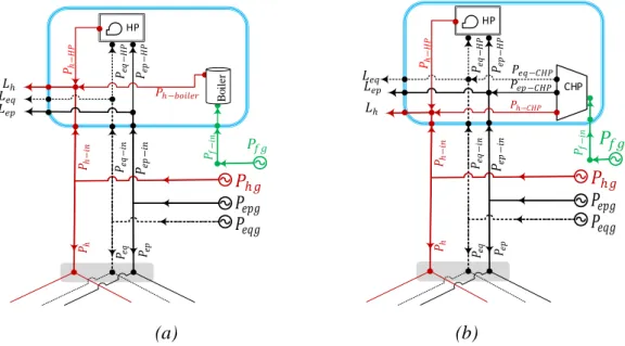
In this paper, an extended representation of an energy hub is used to do a pseudo-dynamic analysis of a MCES. In such representation, the local demands, local generations and coupling technologies are altogether represented by an energy hub. Fig. 1a shows how heat pump and gas boiler can be integrated while Fig. 1b shows the integration of heat pump and CHP inside the coupling system (indicated by a blue rectangle). In both figures, HP represents the heat pump. Pfg, Phg, Pepg and Peqg are local generations of fuel, heat, active electric and reactive electric power respectively while Ph, Pep and Peq represent the heat, active electric and reactive electric power injections into the network respectively. Ph-in, Pf-in, Pep-in and Peq-in are the heat, fuel, active electric and reactive electric power inputs into the coupling system respectively while Lh, Lep and Leq are the heat, active electric and reactive electric demands respectively. Ph-CHP, Pep-CHP and Peq-CHP are the heat, active electric and reactive electric power outputs of a CHP plant while Ph-boiler and Ph-HP represent the heat power outputs from the gas boiler and HP respectively. Pep-HP and Peq-HP, on the other hand, represent the active and reactive electric power consumptions of the HP.
2.1. An energy hub with heat pump and gas boiler
Figure 1(a) shows the integration of HP and gas boiler. The heat pump uses electric power to transfer heat from the colder region to the hotter region. Its performance is expressed in terms of coefficient of performance (COP) which is given by the ratio of heat power transported to the amount active
3 electric power consumed. If the heat pump is running at lagging power factor, it also needs reactive power. Thus, HP can be considered as additional load for electricity network. The gas boiler, on the other hand, is expressed by its thermal efficiency, 𝜂𝑏. The coupling matrix (the details can be referred from) Ref. [10]) for an energy hub with heat pump and gas boiler is derived as shown in equation (1).
HP 𝐿𝑒𝑞 𝐿ℎ 𝐿𝑒𝑝 𝑃ℎ𝑔 𝑃𝑒𝑞𝑔 𝑃𝑒𝑝𝑔 𝑃𝑒𝑝 − 𝑖𝑛 𝑃𝑒𝑞 − 𝑖𝑛 𝑃𝑒𝑝 𝑃𝑒𝑞 𝑃ℎ 𝑃ℎ − 𝑖𝑛 𝑃𝑒𝑝 − 𝐻 𝑃 𝑃ℎ − 𝐻 𝑃 𝑃𝑒𝑞 − 𝐻 𝑃 𝑃ℎ−𝑏𝑜𝑖𝑙𝑒𝑟 Boi le r 𝑃𝑓− 𝑖𝑛 𝑃 𝑓𝑔 HP 𝐿𝑒𝑞 𝐿ℎ 𝐿𝑒𝑝 CHP 𝑃ℎ𝑔 𝑃𝑒𝑞𝑔 𝑃𝑒𝑝𝑔 𝑃𝑓𝑔 𝑃𝑒𝑝 − 𝑖𝑛 𝑃𝑒𝑞 − 𝑖𝑛 𝑃𝑒𝑝 𝑃𝑒𝑞 𝑃ℎ 𝑃ℎ − 𝑖𝑛 𝑃𝑓− 𝑖𝑛 𝑃𝑒𝑝 − 𝐻 𝑃 𝑃ℎ − 𝐻 𝑃 𝑃𝑒𝑞 − 𝐻 𝑃 𝑃𝑒𝑝 −𝐶𝐻𝑃 𝑃𝑒𝑞−𝐶𝐻𝑃 𝑃ℎ−𝐶𝐻𝑃 (a) (b)
Fig. 1 Interaction between different energy carriers at an energy hub: a) with HP and gas boiler b) with HP and CHP. [ 𝐿𝑒𝑝+ 𝑃𝑒𝑝−𝐻𝑃 𝐿𝑒𝑞+ 𝑃𝑒𝑝−𝐻𝑃 √1−𝑝𝑓𝐻𝑃 2 𝑝𝑓𝐻𝑃 𝐿ℎ− 𝑃𝑒𝑝−𝐻𝑃 ∗ 𝐶𝑂𝑃 ] = [ 1 0 0 0 0 1 0 0 0 0 1 𝜂𝑏 ] [ 𝑃𝑒𝑝𝑔− 𝑃𝑒𝑝 𝑃𝑒𝑞𝑔− 𝑃𝑒𝑞 𝑃ℎ𝑔− 𝑃ℎ 𝑃𝑓𝑔 ] , (1)
2.2. An energy hub with heat pump and CHP
A CHP and heat pump can be interconnected as shown in figure 1(b). The CHP produces both active electric power and heat from fuel input. It is expressed by its electrical and thermal efficiencies, 𝜂𝑒𝑙
and 𝜂𝑡ℎ respectively. Depending on whether it is running at lagging or leading power factor (𝑝𝑓𝐶𝐻𝑃),
the CHP either consumes or produces reactive power. The coupling matrix for an energy hub consisting of heat pump and CHP is derived as shown in equation (2).
[ 𝐿𝑒𝑝+ 𝑃𝑒𝑝−𝐻𝑃 𝐿𝑒𝑞+ 𝑃𝑒𝑝−𝐻𝑃 √1−𝑝𝑓𝐻𝑃 2 𝑝𝑓𝐻𝑃 𝐿ℎ− 𝑃𝑒𝑝−𝐻𝑃 ∗ 𝐶𝑂𝑃 ] = [ 1 0 0 𝜂𝑒𝑙 0 1 0 −𝜂𝑒𝑙√1−𝑝𝑓𝐶𝐻𝑃 2 𝑝𝑓𝐶𝐻𝑃 0 0 1 𝜂𝑡ℎ ][ 𝑃𝑒𝑝𝑔− 𝑃𝑒𝑝 𝑃𝑒𝑞𝑔 − 𝑃𝑒𝑞 𝑃ℎ𝑔 − 𝑃ℎ 𝑃𝑓𝑔 ] , (2)
In both equations (1) and (2), power factor is considered to be positive if it is lagging and negative otherwise.
2.3. Constituent equations for load flow modelling
The power mismatch at each hub is generally expressed in terms coupling matrices as shown in equation (3a) [10].
4 [ 𝐿𝑒𝑝(𝑘) 𝐿𝑒𝑞(𝑘) 𝐿ℎ(𝑘) ] − [ 𝐶𝑘−𝑒𝑝(𝑒𝑝) 𝐶𝑘−𝑒𝑝(𝑒𝑞) 𝐶𝑘−𝑒𝑝(ℎ) 𝐶𝑘−𝑒𝑝(𝑓) 𝐶𝑘−𝑒𝑞(𝑒𝑝) 𝐶𝑘−𝑒𝑞(𝑒𝑞) 𝐶𝑘−𝑒𝑞(ℎ) 𝐶𝑘−𝑒𝑞(𝑓) 𝐶𝑘−ℎ(𝑒𝑝) 𝐶𝑘−ℎ(𝑒𝑞) 𝐶𝑘−ℎ(ℎ) 𝐶𝑘−ℎ(𝑓) ] [ 𝑃𝑒𝑝𝑔(𝑘)− 𝑃𝑒𝑝(𝑘) 𝑃𝑒𝑞𝑔(𝑘)− 𝑃𝑒𝑞(𝑘) 𝑃ℎ𝑔(𝑘)− 𝑃ℎ(𝑘) 𝑃𝑓𝑔(𝑘) ] = [ 𝑑𝑃𝑒𝑝(𝑘) 𝑑𝑃𝑒𝑞(𝑘) 𝑑𝑃ℎ(𝑘) ], (3a) where 𝐶 represent the coupling matrix respectively; the subscripts k represent hub number; ep, eq, h, and f indicate active electric, reactive electric, heat and fuel powers, respectively while g represented locally generated power. 𝑑𝑃𝑒𝑝(𝑘), 𝑑𝑃𝑒𝑞(𝑘) and 𝑑𝑃ℎ(𝑘) represent active electric, reactive electric and
heat power mismatches at hub k, respectively.
For an N bus electricity network, the per unit active and reactive power injections at any bus k are given by equations (3b) and (3c), respectively [10].
𝑃𝑒𝑝(𝑘) = ∑𝑁 |𝑉𝑘|
𝑗=1 |𝑉𝑗|(𝐺𝑘𝑗𝑐𝑜𝑠𝜃𝑘𝑗+ 𝐵𝑘𝑗𝑠𝑖𝑛𝜃𝑘𝑗), (3b)
𝑃𝑒𝑞(𝑘) = ∑𝑁 |𝑉𝑘|
𝑗=1 |𝑉𝑗|(𝐺𝑘𝑗𝑠𝑖𝑛𝜃𝑘𝑗− 𝐵𝑘𝑗𝑐𝑜𝑠𝜃𝑘𝑗), (3c) where 𝐺𝑖𝑗 + 𝑗𝐵𝑖𝑗 = 𝑌𝑖𝑗 is an
element of the network admittance matrix of size N by N.
The heat power injection into the network from hub k can be given by equation (3d).
𝑃ℎ(𝑘) = 𝐶𝑝𝑚̇𝑘(𝑇𝑠𝑘− 𝑇𝑟𝑘) , (3d) where 𝑃ℎ(𝑘) is heat power injected (positive for source and negative for load), 𝑚̇𝑘 is mass flow rate flowing from the hub to the supply pipe network
of the DHN (positive for source and negative for load), 𝑇𝑠𝑘 and 𝑇𝑟𝑘 are supply and return temperatures
at node k respectively.
In addition to these coupled equations, there are additional mismatch equations for the hydraulic head and temperature variables as shown in equations (4) to (6). The details of additional equations that are used to solve the temperature and pressure drops in the pipe network can be found in Ref. [10]. 𝑑𝐻𝑖𝑗 = 0 = (𝐻𝑗− 𝐻𝑖− 𝐾𝑖𝑗𝑚̇𝑗𝑖|𝑚̇𝑗𝑖|), (4)
𝑑𝑇𝑠𝑖 = 0 = (∑𝑗∈𝑖𝑛𝑇𝑠−𝑗𝑖𝑚̇𝑗𝑖 − 𝑇𝑠𝑖(𝑜)∑𝑗∈𝑖𝑛𝑚̇𝑗𝑖), (5)
𝑑𝑇𝑟𝑘= 0 = (∑𝑗∈𝑖𝑛𝑇𝑟−𝑗𝑘𝑚̇𝑗𝑘− 𝑇𝑟𝑘(𝑜)∑𝑗∈𝑖𝑛𝑚̇𝑗𝑘), (6)
where: 𝑑𝐻𝑖𝑗 is the hydraulic head mismatch corresponding to pipe connecting hub i (with pressure
head 𝐻𝑖) and hub j (with hydraulic head 𝐻𝑗); 𝐾𝑖𝑗 is the pressure resistance coefficient of a pipe
connecting hubs i and j; 𝑑𝑇𝑠𝑖 is the supply temperature mismatch at temp-return hub i; 𝑑𝑇𝑟𝑘 is the return temperature mismatch at temp-supply hub k; 𝑚̇𝑗𝑖 and 𝑚̇𝑗𝑘 are mass flow rates flowing from node j to node i and from node j to node k, respectively (they include mass flows from hubs i and k as well if the flows are from the hub into the corresponding nodes); s and r indicate the supply and return pipe networks of the DHN; 𝑇𝑠−𝑗𝑖 is the temperature of the water flowing from node j to node i as measured at node i on the supply pipe network; 𝑇𝑟−𝑗𝑘 is the temperature of water flowing from node j to node k, as measured at node k on the return pipe network; 𝑇𝑠𝑖(𝑜) and 𝑇𝑟𝑘(𝑜) are the outgoing supply temperature at node i and outgoing return temperature at node k, respectively).
Once all the equations are formulated in per unit system (the details can be referred from Ref. [10]), the overall load flow problem is then solved as a single problem using the Newton-Raphson iteration method. The values of all parameters during each simulation hour are used as initial values for the next hour simulation. By doing so, the pseudo dynamic variation of different network variables are analysed. The variables of interest in the load flow solution are voltage magnitude, voltage angle, supply temperature, return temperature, hydraulic heads at each node, nodal mass flow rates and pipe mass flow rates. At a given hub, some of the variables might be known while the others are unknown. The objective of the load flow study is to solve for the unknown variables using the known variables.
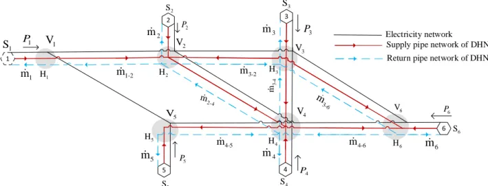
5 A six hub case study (as shown in Fig. 2.) is considered for the pseudo dynamic simulation. The solid line without arrow (black) represents the electricity network. The solid line with arrow (red), on the other hand, represents the supply pipe network of heating network while the dotted line with arrow (blue) represents the return pipe network of the heating network. Each hexagon represents an energy hub consisting of local production of heat, electricity and/or fuel, demands and energy conversion devices. Hub 1 is considered as a slack hub from which the deficit in each carrier power balance is compensated from the neighbourhood or bigger network. It also acts as a point of export to the neighbourhood should the district network have excess power than the required. The slack hub is indicated by dotted hexagon. Hub 2 is a consumer hub with residential demands of both electricity and heat demands. Hub 3 consists of a CHP and heat pump technologies together with fuel source. Automatic voltage regulator is assumed to keep the magnitude of voltage at this hub at unity. There is a residential demand of both electricity and heat at Hub 4. Heat pump and gas boiler are considered at this hub. Hub 5, on the other hand, has a 200kW peak solar PV generation plant. Hub 6 is associated with commercial load profile (small hotel). It should be noted that even though Hubs 1, 3 and 5 do not have connected consumers, there is still electricity demand at Hub3 due to the CHP and HP technologies. Demand profiles for both electricity and heating networks are taken for a residential and commercial building in Idaho, USA from the source [11]. These profiles are taken only for illustration purpose to demonstrate the capacity of the tool proposed in handling pseudo dynamic simulation of a network consisting of different energy technologies. Similarly, all heating demands are assumed to be supplied through the DHN. This means that the DHN is assumed to run throughout the year. Table 1 summarises annual demand profile for each carrier and for overall network.
1 2 2 m m 3 4 m 4 -2 m 3 S 1 S 4 S 2 S 1 V 2 V 3 V 4 V 1 P 2 P 3 P 4 P 5 4-m Electricity network
Supply pipe network of DHN Return pipe network of DHN
5 m 3-2 m 1-2 m 5 P 5 S 1 m 3-6 m 4-6 m 6 m 6 P 6 S 3-4 m 4 H 6 H 5 H 1 H H2 H3 6 V 5 V
Fig. 2. The layout of the heating and electricity network considered as a case study. Table 1: Summary of the demand profile considered in the case study
Hub Electricity Heating Remark
Active Reactive Total
(MWh) Peak (kW) Total (MWh) Peak (kW) Peak (kvar) 2 203.559 69.61 43.16 352.73 168.22 Residential
3 164.955 25 59.61 0 0 Heat pump and CHP
4 713.719 174.23 67.64 704.49 318.41 Residential & heat pump
5 0 0 0 0 0 Solar PV plant
6 963.263 203.81 97.83 231.59 122.21 Small hotel All 2,045.5 426.41 227.97 1,288.8 595.81 Whole network
6 The details of the network parameters are included in Appendix A. Standardized transmission line parameters (ACSR Ostrich type) and typical values of distribution transformers parameters (4.16kV, 1MVA) are taken from a reference [12]. Similarly, standardized parameters of district heating pipes (DN 50 with series II insulation layer) are taken from isoplus® [13]. The peak rating of the CHP is 87.5kWe and 100kWth with efficiency of 35% and 40%, respectively. The CHP runs at a lagging power factor of 0.86. The gas boiler has a thermal efficiency of 85% with rated thermal output of 42.5kW. The rated electrical power of the heat pump at Hub 3 is 25kW with a COP of 3.5 at 0.9 lagging power factor. The heat pump at Hub4, on the other hand, is rated at 35kW electrical power with a COP of 4.0 at 0.85 lagging power factor.
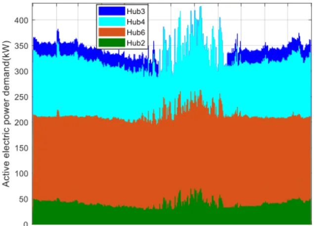
Figures 3 – 5 shows the demand profiles. The heat pump at Hub4, the boiler at Hub4 and the CHP at Hub3 are scheduled following the heat demand profile. The boiler runs during the peak-heat-demand periods (i.e. from Jan 1st to Mar 15th and the last two weeks of December). The heat pump at Hub4 is assumed to be operated year round (covering the base heating load) while the heat pump at Hub3 is assumed to be turned off from mid of June to mid of September. Similarly, the CHP plant at Hub3 is scheduled to be turned off between mid of May and the end of October. The effect of scheduling these technologies on the electric demand profile can be seen in figures 4 and 5. Supply temperature of hubs acting as heat source is taken to be 85oC while the return temperature from hubs that consumes heat is assumed to be 35oC.
Fig. 3: Heat demand profile Fig. 4: Active electricity demand
7
4. Results and Discussion
4.1. Analysis for the overall network
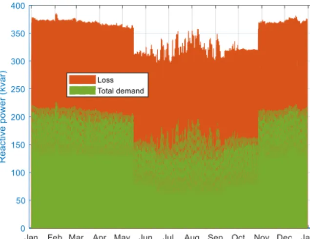
Fig. 6 shows the total heat power demand and the heat power lost in the network. It can be seen that the peak demand occurs in February. The annual heat power energy lost in the network is 1,624.1MWh which corresponds to 126% of the demand. This shows that there is significant amount of heat loss in the network. As a percentage of heat demand, the heat loss in the network is higher in summer than winter. This could be due to lower mass flow rate of water (nearly zero) flowing in the network during summer. Similarly, the active electric power lost in the electricity network is plotted in Fig. 7. The total active electric energy lost is 434.58MWh, which corresponds to 21.25% of the demand. Fig. 8, on the other hand, shows the reactive power consumed in the network. It can be seen that the magnitude of reactive power consumed in the network remains more or less the same even though the reactive power demand at Hub 3 is changing when the CHP plant is switched off. Tis because of the consideration of Hub3 as a voltage controlled hub where there is sufficient reactive power generation capacity. To keep the voltage magnitude at this hub constant, the net injected reactive power should remain the same. Hence, any reactive load at Hub3 is supplied mainly from the reactive power generated at the same hub. Because of this, the reactive power flow in the network and the corresponding loss remains more or less the same even though the demand at hub 3 is changing.
Fig. 7: Active electricity lost in the network Fig. 8: Reactive electricity lost in the network
Fig. 9: Heat power generated Fig. 10: Active electric power generated The amount of generated and imported heat power is plotted in Fig. 9. The imported heat is sometimes negative which means that the network is exporting the excess heat energy to the neighbourhood. The
8 total amount of imported heat energy is 640.74MWh (with a peak value of 535.64kW) while the total amount of exported heat energy is 103.24MWh (with peak value of 156.71kW). Installing heat storage units may help to reduce the imported heat energy by storing the excess heat produced. The heat energy produced at Hub4 is 1,318.2MWh (91.48MWh from the gas boiler and 1,226.4MWh from the heat pump). On the other hand, 1,057.2MWh heat energy is produced at Hub3 (479.9MWh from the CHP and 577.34MWh from heat pump). The boiler consumed 108.05MWh of fuel while the CHP consumed 1,199.75MWh gas.
The generated active electricity power and the imported quantity is shown in Fig. 10. A total of 765.58MWh (419.91MWh from the CHP and 345.67MWh from solar PV) is produced in the network while 1,722.2MWh is imported from the neighbourhood. This shows that the sizes of distributed generation technologies considered in the case study are insufficient from the electrical demand point of view.
In summary, 1,307.8MWh of fuel, 640.74MWh of imported heat, 1,722.2MWh imported active electricity and 345.67MWh active electricity from solar PV are used to supply the demands of 2,045.5MWh of active electricity and 1,288.8MWh of heat.
4.2. Analysis at hub level
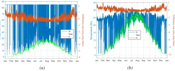
The analysis on different hub parameters can also be done based on the pseudo dynamic simulation. Fig. 11, for example, shows the variation of temperature and mass flow rate throughout the year for Hub1. The supply temperature variation is depicted in Fig. 11(a) while the return temperature variation is shown in Fig. 11(b). It can be observed that both of the supply and return temperatures remain above or equal to the soil temperature, but never below 1oC to avoid freezing of water inside
network pipes. The soil temperature is taken 10cm below the surface of the earth. The temperature approaches to the soil temperature when the mass flow rate is close to zero. It is assumed that there is a backup heat source (locally or from the neighbourhood) which can be used during shortage time to supply heat at 85oC. These shortage times are indicated by positive mass flows (same as the direction assumed in Fig. 2). During excess heat production, however, the mass flow rate changes direction and, hence the supply temperature at Hub1 will be determined by the network while the return temperature can be assumed to be equal to the soil temperature, but greater than or equal to 1
oC (see Fig. 11).
(a) (b)
Fig. 11: Temperature and mass flow profile at Hub1 (a) supply side; (b) return side of DHN
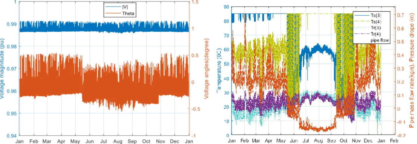
Hub based analysis can also be done for electrical parameters such as voltage magnitude and voltage angle. Fig. 12 shows these parameters at Hub5 where there is solar PV. Even though the variation in voltage magnitude is very small, it looks that the pattern follows the output of the solar PV. The
9 voltage angle, on the other hand, seems to be affected by the CHP plat scheduling as it can be seen by lower values between the mid of May and the end of October.
Fig. 12 Voltage magnitude and angle at Hub5 Fig. 13 End point water temperature at pipe 3-4
4.3. Analysis at branch level
Additional analysis can be done for each branch of the electricity and heating networks. As an example, the variation of water temperature on the pipe connecting Hub3 and Hub4 is shown in Fig. 13. When the mass flow rate is positive, the supply temperature at the end of the pipe near to Hub3 (Ts(3)) is greater than the other end (Ts(4)).Whenever the mass flow rate becomes negative, the supply
temperature at the end point located near to Hub4 becomes greater than the end point located near to Hub3. The same is true for the return pipe, but opposite to the supply pipe as the water flows in opposite direction. It can also be noted that the temperature drop is function of the water temperature and, hence, there is less temperature drop in the return pipe as compared to the supply pipe network.
5. Conclusions
In this paper, a load flow model based on an extended energy hub approach is used to do a pseudo dynamic simulation on coupled electricity and heating networks. Distributed generations such as CHP, solar PV, gas boilers and heat pumps are considered in the simulation. It has been observed that the way CHP and heat pumps are operating affects both networks. It is also found out that sizing the generation capacities of coupling technologies based on one type of demand profile could lead to undersized or oversized generation capacity for the other network. The losses in the heating networks should also be given due attention as they may become more than the actual demand in some situations.
The thermal parameters at Hub1 can be further developed together with the peak power and total energy imported and exported in order to design underground thermal storage system as there is no nationwide heating network to where the excess production can be exported. In addition, as the tool shows all network parameter variations throughout the year, it can be further used as part of optimization tools to determine the economical size of different energy technologies. In the case of DHN, for instance, source temperatures, operational periods and the sizes of CHPs and HPs together with the possibility of load shaving can be considered as decision variables in the optimization process. The details of the voltage, temperature and mass flow rate profiles at different parts of the network can also be further analysed for operational and control strategies.
Acknowledgments
The research presented is performed within the framework of the Erasmus Mundus Joint Doctorate SELECT+ program ‘Environomical Pathways for Sustainable Energy Services’ and funded with support from the Education, Audiovisual, and Culture Executive Agency (EACEA)
(FPA-2012-10 0034) of the European Commission. This publication reflects the views only of the author(s), and the Commission cannot be held responsible for any use, which may be made of the information contained therein.
Nomenclature
b Susceptance of transmission line (S)
𝐶𝑘−𝛿(𝛾) Coupling coefficient at hub k relating generation type 𝛾 with load type 𝛿
Cp Specific heat capacity of water (J/Kkg)
D,D1 Internal diameter of a pipe (m)
D3 Outer diameter of insulating material(m) DHN District Heating Network
∆𝑇 Temperature difference (K)
e Internal surface roughness of a pipe (m)
H Hydraulic head (m)
K Pressure resistance coefficient (m.s2/kg2)
L Length (m)
Lep Electricity active power demand (W)
Leq Electricity reactive power demand (var)
Lh Heat power demand (W)
𝑚̇ Mass flow rate from a hub (kg/s) 𝑚̇𝑖𝑗 Mass flow rate from node i to j (kg/s) MCES Multi carrier energy system
Pep Electricity active power injection (W)
Pepg Electricity active power generated (W)
Peq Electricity reactive power injection (var)
Peqg Electricity reactive power generated (var)
Pf Fuel power injection (W)
Pfg Fuel power generation (W)
Ph Heat power injection (W)
Phg Heat power generation (W)
R Resistance of a transmission line (Ω) S Locally generated power
T Temperature (K)
t1 Thickness of carrier pipe (m)
t3 Thickness of outer jacket (m)
𝜃 Voltage angle (degree)
V Voltage (V)
X Reactance of a transmission line (Ω) Xs Transformer leakage reactance (Ω)
Y Bus admittance matrix
Z Depth of pipe from the surface of earth to the centre of pipe (m) Subscripts
11
i, j, k Hub numbers
r Return pipe of DHN
s Supply pipe of DHN
References
[1] Liu X, Mancarella P. Modelling, assessment and Sankey diagrams of integrated electricity-heat-gas networks in multi-vector district energy systems. Appl Energy 2016;167:336–352.
[2] Geidl M, Andersson G. Optimal Power Flow of Multiple Energy Carriers. IEEE Trans Power Syst 2007;22:145–55. doi:10.1109/TPWRS.2006.888988.
[3] Lund H, Werner S, Wiltshire R, Svendsen S, Thorsen JE, Hvelplund F, et al. 4th Generation District Heating (4GDH): Integrating smart thermal grids into future sustainable energy systems. Energy 2014;68:1–11. doi:10.1016/j.energy.2014.02.089.
[4] Geidl M. Integrated modeling and optimization of multi-carrier energy systems. PhD. TU Graz, 2007.
[5] Liu X, Wu J, Jenkins N, Bagdanavicius A. Combined analysis of electricity and heat networks. Appl Energy 2016;162:1238–50. doi:10.1016/j.apenergy.2015.01.102.
[6] Shabanpour-Haghighi A, Seifi AR. An Integrated Steady-State Operation Assessment of Electrical, Natural Gas, and District Heating Networks. IEEE Trans Power Syst 2016;31:3636– 47. doi:10.1109/TPWRS.2015.2486819.
[7] Boulos PF, Lansey KE, Karney BW. Comprehensive Water Distribution Systems Analysis Handbook for Engineers and Planners. American Water Works Assn; 2006.
[8] Mohammadi S, Bojsen C, Milan C. Identifing the Optimal Supply Temperature in District Heating Networks-a Modelling Approach. Proc. 14th Int. Symp. Dist. Heat. Cool., Swedish District Heating Association; 2014.
[9] Fedorov M. Parallel implementation of a steady state thermal and hydraulic analysis of heat exchanger. Pomiary Autom Kontrola 2009;R. 55, nr 10:815–9.
[10] Ayele GT, Haurant P, Laumert B, Lacarrière B. An extended energy hub approach for load flow analysis of highly coupled district energy networks: Illustration with electricity and heating. Appl Energy 2018;212:850–67. doi:10.1016/j.apenergy.2017.12.090.
[11] Comercial and residential hourly load profile- Available at:<https://openei.org/datasets/files/961/pub/> [accessed January 8, 2018].
[12] Glover JD, Sarma MS, Overbye T. Power System Analysis & Design, SI Version. Cengage Learning; 2012.
[13] isoplus: Flexible and rigid pipes and pipeline systems: isoplus - isoplus Fernwärmetechnik. Available at: <http://www.isoplus-pipes.com/> [accessed September 3, 2017].
Appendices
A: Branch parameters
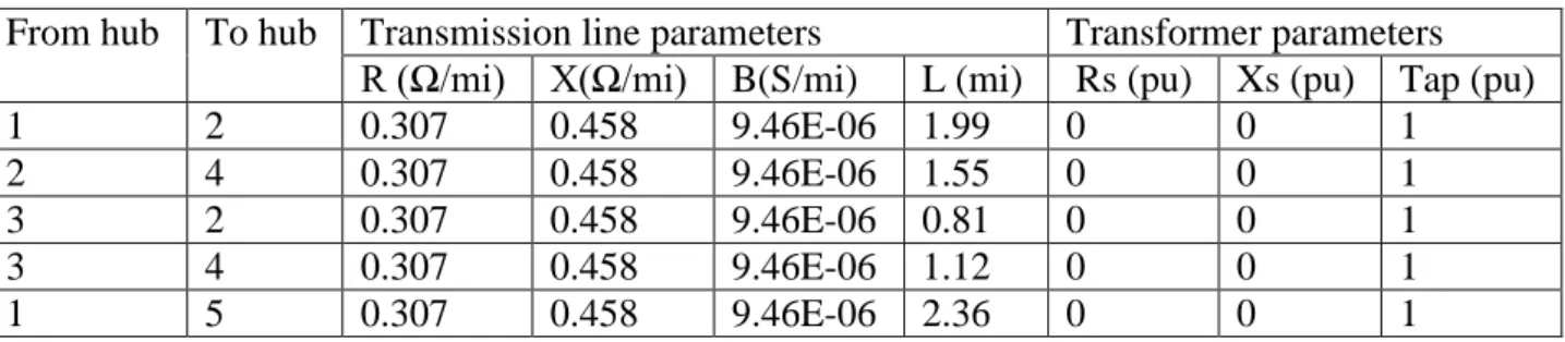
Table A-1: Transmission line and transformer parameters for the electricity networks From hub To hub Transmission line parameters Transformer parameters
R (Ω/mi) X(Ω/mi) B(S/mi) L (mi) Rs (pu) Xs (pu) Tap (pu)
1 2 0.307 0.458 9.46E-06 1.99 0 0 1
2 4 0.307 0.458 9.46E-06 1.55 0 0 1
3 2 0.307 0.458 9.46E-06 0.81 0 0 1
3 4 0.307 0.458 9.46E-06 1.12 0 0 1
12
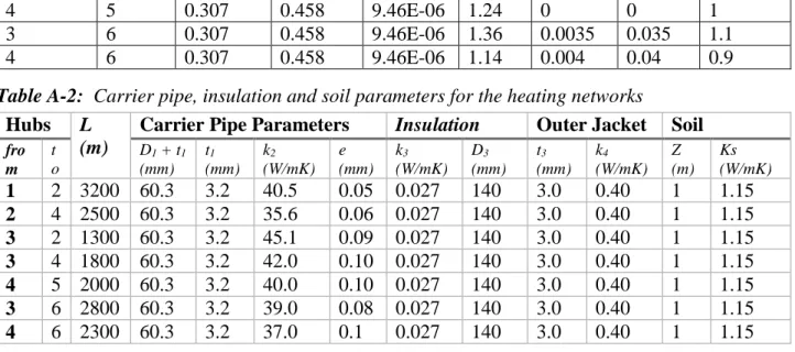
4 5 0.307 0.458 9.46E-06 1.24 0 0 1
3 6 0.307 0.458 9.46E-06 1.36 0.0035 0.035 1.1
4 6 0.307 0.458 9.46E-06 1.14 0.004 0.04 0.9
Table A-2: Carrier pipe, insulation and soil parameters for the heating networks
Hubs L
(m)
Carrier Pipe Parameters Insulation Outer Jacket Soil
fro m t o D1 + t1 (mm) t1 (mm) k2 (W/mK) e (mm) k3 (W/mK) D3 (mm) t3 (mm) k4 (W/mK) Z (m) Ks (W/mK) 1 2 3200 60.3 3.2 40.5 0.05 0.027 140 3.0 0.40 1 1.15 2 4 2500 60.3 3.2 35.6 0.06 0.027 140 3.0 0.40 1 1.15 3 2 1300 60.3 3.2 45.1 0.09 0.027 140 3.0 0.40 1 1.15 3 4 1800 60.3 3.2 42.0 0.10 0.027 140 3.0 0.40 1 1.15 4 5 2000 60.3 3.2 40.0 0.10 0.027 140 3.0 0.40 1 1.15 3 6 2800 60.3 3.2 39.0 0.08 0.027 140 3.0 0.40 1 1.15 4 6 2300 60.3 3.2 37.0 0.1 0.027 140 3.0 0.40 1 1.15