Science Arts & Métiers (SAM)
is an open access repository that collects the work of Arts et Métiers Institute of
Technology researchers and makes it freely available over the web where possible.
This is an author-deposited version published in:
https://sam.ensam.eu
Handle ID: .
http://hdl.handle.net/10985/15357
To cite this version :
Emmanuel COTTANCEAU, Olivier THOMAS, Philippe VÉRON, Marc ALOCHET, Renaud
DELIGNY - A finite element/quaternion/asymptotic numerical method for the 3D simulation of
flexible cables - Finite Elements in Analysis and Design - Vol. 139, p.14-34 - 2018
A finite element/quaternion/asymptotic numerical method for the 3D
simulation of flexible cables
Emmanuel Cottanceau
a,b, Olivier Thomas
a,*, Philippe Véron
a, Marc Alochet
b,
Renaud Deligny
baArts et Métiers ParisTech, LSIS UMR CNRS 7296, 8 bd. Louis XIV, 59046 Lille, France bTechnocentre Renault, 1 av. Du Golf, 78084 Guyancourt, France
A R T I C L E I N F O Keywords:
Cables
Finite element method Asymptotic numerical method Quaternions
A B S T R A C T
In this paper, a method for the quasi-static simulation of flexible cables assembly in the context of automotive industry is presented. The cables geometry and behavior encourage to employ a geometrically exact beam model. The 3D kinematics is then based on the position of the centerline and on the orientation of the cross-sections, which is here represented by rotational quaternions. Their algebraic nature leads to a polynomial form of equi-librium equations. The continuous equations obtained are then discretized by the finite element method and easily recast under quadratic form by introducing additional slave variables. The asymptotic numerical method, a powerful solver for systems of quadratic equations, is then employed for the continuation of the branches of solution. The originality of this paper stands in the combination of all these methods which leads to a fast and accurate tool for the assembly process of cables. This is proved by running several classical validation tests and an industry-like example.
1. Introduction
During the last decades, the room available in car vehicles (e.g. in engine compartment) has plummeted because of the rapid development of on-board electronics. As a result, a need for very accurate numerical tools for design has appeared in automotive industry. In the meantime, a fast computation is necessary so that design duration remains suitable for industry. In this context, flexible pieces represent an outstanding challenge since, unlike most of car pieces, they cannot be modeled as rigid body solids in CAD software. This paper focuses on a specific type of flexible piece, namely electrical cables. Cables have a complex struc-ture. A wire is made up of copper filaments wrapped in an elastomer duct. These wires are most of the time gathered in bundles which are themselves surrounded by various protections such as tape, PVC tube …Moreover, the full cable is often constituted of several drifted cable pieces forming a system with a complex geometry.
Due to its slender shape and its flexibility, one can consider a simple cable as a beam undergoing large displacements and large rotations. There exist several theories accounting for nonlinear beams, see Refs. [1–3]. The most widely used theory is the geometrically exact beam model whose founding principles were established by Reissner[4,5] and further generalized by Simo[6]. Various finite element
formula-* Corresponding author.
E-mail address:olivier.thomas@ensam.eu(O. Thomas).
tions (FEM) have been presented to solve these equations numerically. The notable works of[7–11]and more recently[12,13] can, among others, be listed.
At the heart of all these formulations, the rotation parameteriza-tion is of paramount importance in the numerical models. The 3D rota-tions modeling indeed is not an easy task especially when computa-tional efficiency is sought. The rotacomputa-tional vector-like parameterization used by many authors features only 3 parameters (minimum set in 3D). However, as no parameterization of less than 4 parameters can be singularity-free[14], this choice poses several numerical limitations and lacks robustness. A powerful alternative consists in using quater-nions, a set of 4 singularity-free parameters. Firstly used only for stor-age in the numerical models, Zupan et al.[12]have recently shown their utility when used as primary variables. They also have devel-oped a model without rotation matrices exploiting the high potential of quaternion algebra, and very efficient for numerical purposes[15]. In addition, quaternions offer an original description of rotations since they substitute the usual trigonometric functions by algebraic variables and lead to polynomial equilibrium equations.
The finite element method, very adapted to the assembly of com-plex geometries such as electrical cables ones, is applied to the con-tinuous equilibrium equations. The algebraic system obtained is then
https://doi.org/10.1016/j.finel.2017.10.002
Received 23 June 2017; Received in revised form 21 September 2017; Accepted 3 October 2017 Available online XXX
generally solved by a classical predictor-corrector method (PCM)[16]. Even if the appearance of arc-length methods[17] has considerably enhanced the robustness of this type of method, they often require to choose a step size which may be very tricky for the user. A sufficiently small step size allows to compute even highly nonlinear part of equi-librium branches but in return may impractically increase the compu-tation time, while a larger step size may spoil the convergence. Taking advantage of the polynomial form of the system of equations obtained when using quaternion parameters an alternative consists in replacing the PCM by the asymptotic numerical method (ANM) firstly presented by Damil and Potier-Ferry[18]and by Cochelin[19]. The ANM is a very powerful solver for quadratic problems and it overcomes all the drawbacks of the PCM. This technique indeed is very robust, does not require any tuning parameters and is thus well suited for an industrial use. In addition, Cochelin and Medale[20]have equipped the method with a bifurcation detector and improved its efficiency in the vicinity of bifurcation points.
Combining quaternions with the ANM has already been set up on a rod model discretized with a finite difference scheme by Lazarus et al.[21], which have got very promising results. We propose here to set up the technique on the finite-element based geometrically exact beam model, in what constitutes the main originality of this paper. Val-idations and illustrations of the method on very intricate problems are provided and discussed. A critical evaluation and future researches are presented by way of conclusion.
2. Governing equations
In this section, the classical quasi-static formulation of the geomet-rically exact beam model, based on the rotation vector, is firstly pre-sented. It enables to explain all the main ingredients of the model and to discuss their physical meaning. Secondly, the equations are modified by using quaternions instead of the rotation vector. This leads to the formulation which serves our numerical model, presented in part3.
2.1. The geometrically exact beam model
In the geometrically exact beam model, a beam is described by defining a family of cross-sections whose centroids form a curve called
the centerline of the beam. The kinematic variables essential to this description are introduced following the notations used in Ref.[22]. Let us consider a beam of initial length L, with an arbitrary cross-section Ω, as depictedFig. 1. Let (u1, u2, u3)be a fixed Cartesian (global) frame.
The current position of the centerline in this frame is described by the vector field x0(s) which is a function of the curvilinear abscissa s ∈ [0, L]
along the beam axis. A material (local) frame (e1(s), e2(s), e3(s)) is
intro-duced to define the cross-section at abscissa s. The vectors e2 and e3
span the cross-section while the vector e1remains normal to the
cross-section for every deformed configurations. It is essential to note that e1 is not necessarily tangent to the centerline of the beam such that shear deformation is taken into account (Timoshenko model). The reference configuration is chosen such that the beam is unstressed. However, in this state, the reference position of the centerline is an arbitrary curve and not necessarily a straight line, thus accounting for the initial curva-ture of the beam. Its initial position is then a function of s denoted X0(s),
such that the displacement of any point of the centerline is x0(s) − X0(s).
Similarly, the material frame in the reference configuration depends on s and is denoted (E1(s), E2(s), E3(s)). To end up with the definition
of the kinematic variables, let us introduce the two rotation operators
R0(s) and R(s) which depict the orientation of the material frames in
the global frame in the initial and in the current configuration respec-tively, that being Ei(s) = R0(s)uiand ei(s) = R(s)ui, i ∈ {1, 2, 3}. As R0(s)
defines the initial curvature of the beam it is constant through the defor-mation. With these notations, the position vector in the spatial frame of any point M′of the undeformed beam located in the section at s writes
X(s, X2, X3) =X0(s) + R0(s)Y(X2, X3), (1)
where Y(X2, X3) = [0 X2 X3]T is the material position of M′ in
the cross-section. Under the assumption that cross-sections remain plane and do not undergo any deformations along the transformation,
Y(X2, X3)is constant and M′after deformation becomes M″whose
posi-tion is given by
x(s, X2, X3) =x0(s) + R(s)Y(X2, X3). (2)
The current configuration of the beam is then completely characterized by the position of the centerline x0(s) and the orientation of the
cross-sections R(s). One recovers here that the kinematic variables depend solely on the curvilinear abscissa s as for any beam model. As it is
clearly implied, the dependency in s is dropped in the following. Fur-thermore, the derivative with respect to s is from now on denoted with the prime symbol′.
For any rotation operator R, it is shown that the matrix RTR′ is
skew-symmetric[22]. Any 3 × 3 skew-symmetric matrix A is made of only 3 independent components which can be gathered in a vector
a = vect(A) = [a1 a2 a3]T. The skew-symmetric matrix associated to
a is denoted̃a and is equal to:
̃a = ⎡ ⎢ ⎢ ⎢ ⎣ 0 −a3 a2 a3 0 −a1 −a2 a1 0 ⎤ ⎥ ⎥ ⎥ ⎦ . (3)
With these notations and hypothesis, the material translational and rotational strain measures are equal to[23].
𝚪 =[Γ1Γ2Γ3]T=RTx′ 0−𝚪0 (4a) K =[𝜅1𝜅2𝜅3 ]T =vect(RTR′) −K 0, (4b)
where the intrinsic translational strain𝚪0=RT0X′0=u1and the intrinsic
rotational strain K0=vect(RT
0R ′
0)solely depend on the initial
configu-ration of the beam. Let us point out that in the reference configuconfigu-ration, the strain measures𝚪 and K are both equal to 0: the assumption of an initially unstressed configuration is thus well recovered by these mea-sures definition.
To interpret these measures, let us consider the straightforward case in which the beam centerline is a straight line in the reference configu-ration. The intrinsic strains then obey𝚪0=u1and K0=0. x′0(s) is, by
definition, a vector tangent to the centerline of the beam at abscissa s in the current configuration. In expression(4a), the operator RTmaps back this vector projection from the material frame to the fixed frame. The measure𝚪 then consists in comparing this quantity to its reference value u1. A fully equivalent interpretation is made by recalling that
the scalar product of 2 vectors may be geometrically interpreted as the projection of one vector in the direction of the other. It follows that Γ1=eT 1x ′ 0−1, Γ2=eT2x ′ 0and Γ3=eT3x ′
0are the comparison of the
pro-jection of x′
0(s) on the material frame to e1in the 3 material directions.
As the beam is parameterized by the curvilinear abscissa in the initial configuration, the norm of x′
0(s) is equal to 1 if the length of the
center-line remains unchanged, is greater than 1 in case of elongation of the centerline and smaller than 1 in case of shortening. With regard to all these observations, we eventually infer that Γ1is the axial strain of the
neutral axis, while Γ2and Γ3represent the shear strains in directions
e2and e3.
In the case of a pure rotational transformation R, RTR′represents
the gradient of the transformation along the beam axis. As this quan-tity is a skew-symmetric matrix, it is equivalent to write RTR′Y and
vect(RTR′) ×Y = K × Y. It follows directly that in(4b)𝜅
1depicts the
torsional strain while𝜅2and𝜅3represent the curvature strains around
e2and e3respectively.
The expression of the aforementioned rotation operator R is gener-ally obtained from a reduced representation. The choice of this rep-resentation is actually a crucial issue since various criteria compete against each other to get the best set of parameters: numerical efficiency (number of parameters), mathematical form, existence of singularities, geometric interpretation. Let us recall that any 3D rotation of a rigid body solid is made up of 3 independent parameters. The 3-parameters rotational vector𝝑 presented in this paragraph thus constitutes the
min-imal set of parameters. We choose it here for its easy geometrical inter-pretation since it is defined by
𝝑 = 𝜗n =[𝜗1 𝜗2 𝜗3
]T
, (5)
for a rotation of angle𝜗 around the unit axis n. The rotation operator
then writes in terms of this parameterization as[22]
R(𝝑) = I3+sin(𝜗𝜗)̃𝝑 + 1 − cos(𝜗)𝜗2 ̃𝝑̃𝝑. (6)
2.2. Virtual work principle
Using the quantities introduced in the previous section and the Cartesian rotational vector𝝑 defined in(5)as rotational parameters, the virtual work principle for a 3D shear elastic beam is stated here. Following Reissner’s work[4,5]and the generalization of Simo[6], it writes ∫ L 0 (N ·𝛿𝚪 + M · 𝛿K) ds = ∫ L 0 ( ne·𝛿x0+me·𝛿𝝑 ) ds +[Ne·𝛿x0]L0+[Me·𝛿𝝑]L0, (7) with the generalized stress resultant in force and moment N and M, the external applied force and moment per unit length neand me, the
external end force and moment Neand Meand the virtual positional
and rotational vectors𝛿x0 and𝛿𝝑. The left-hand of the equation is
the opposite of the virtual work of internal forces −𝛿iand the right-hand is the virtual work of external forces𝛿e. N = [N T2T3]T and
M = [MtM2M3]Tare work conjugates to the virtual translational strain
𝛿𝚪 and the virtual rotational strain 𝛿K respectively. Therefore, N stands
for the axial force resultant, T2and T3the transverse force resultants
in respective directions e2and e3, Mtthe torsional moment and M2and
M3the bending moments around axis e2and e3.
In the scope of this paper, only linear elastic materials are consid-ered. In this particular case, the stress-strain relationship states pro-portionality between stress resultant vector𝚺 = [MTNT]T and strain
resultant vector = [𝚪TKT]Tthat be
𝚺 = C = diag(CN, CM). (8)
In(8), CN=diag(EA, GA2, GA3)and CM=diag(GJ, EI2, EI3)are the two
3 × 3 stress-strain submatrices corresponding solely to the force compo-nents and the moment compocompo-nents respectively. In these expressions,
E and G are respectively the Young’s modulus and the shear modulus
of the material; A is the cross-sectional area; A2and A3are the shear
areas in directions e2and e3; I2, I3are the second moments of area with respect to axes e2, e3; J is the polar moment of area.
Let us notice that this model can take into account the case of the origin of the material frame not being on the centerline effortlessly. In this case, out-of-diagonal terms simply appear in the stress-strain matrix
C.
Finally, the virtual strains in(7)are given in terms of the kinematic variables by the equations[22]:
𝛿𝚪 = RT𝛿x′ 0+ ̃RTx′0T𝛿𝝑 = R T𝛿x′ 0+ (̃𝚪 + ̃𝚪0)T𝛿𝝑, 𝛿K = (RTR′T + T′)𝛿𝝑 + T𝛿𝝑′= ((̃ K + ̃K0)T + T′)𝛿𝝑 + T𝛿𝝑′. (9)
In(9), T is a tangent operator which can be expressed as a function of
𝝑 only under the form: T = I3+cos(𝜗) − 1 𝜗2 ̃𝝑 + 1𝜗2 ( 1 −sin(𝜗) 𝜗 ) ̃𝝑̃𝝑. (10)
2.3. Strong form of equilibrium equations
Introducing expressions(9)into the virtual work principle(7), inte-grating by parts with some rearranging and using the fundamental lemma of calculus of variations lead to the following equilibrium equa-tions: { (RN)′+ne=0, (RM)′+x′ 0× (RN) + me=0, ∀s ∈ [0 L] (11)
along with the natural boundary conditions {
RN − Ne=0 at s = 0, L, RM − Me=0 at s = 0, L,
or the essential boundary conditions {
x0=xd at s = 0, L,
𝝑 = 𝝑d at s = 0, L, (13)
where xdand𝝑dare respectively imposed positions and rotations. 2.4. Quaternion parameterization of rotations
As explained at the end of paragraph 2.1, the choice of rota-tion parameters is of paramount importance in numerical models. In a total Lagrangian framework (i.e. using total rotations), the rota-tional vector 𝝑 prevents from having angles greater than 2𝜋. It is clear from equation(10)that the tangent operator T indeed becomes rank-deficient around 2𝜋-angles and leads to a singularity. Procedures exist to circumvent this flaw[9], however, we find it more expedi-ent to use an other parameterization not requiring any special pro-cedure. As demonstrated in Ref.[14], the minimal set of parameters avoiding all singularities is made up of 4 parameters. With regard to this principle, the 4-parameters quaternions appear as an optimal choice for the representation of rotations. In addition, quaternions feature a special algebra totally equivalent to the algebra of rota-tion operators but which proves computarota-tionally more efficient[24]. Finally, they offer a polynomial representation of rotations in com-parison to classical trigonometric ones. We will show in the following part how this property is used as a leverage in our numerical solu-tion.
The next developments of this paragraph aim at giving the funda-mentals on quaternions necessary to the comprehension of the method. The interested reader may consult for instance[25]for more details. The notations of[12]on quaternion algebra are used here. A quater-nion̂a is defined by
̂a = a0+ia1+ja2+ka3, (14)
where a0, a1, a2, a3∈ℝ and the imaginary numbers i, j and k are linked
by the identities
i2=j2=k2=ijk = −1. (15) 1, i, j and k form a basis of the set of quaternions, denotedℍ. As a result, a quaternion may also be seen as an element of the four-dimensional Euclidean linear spaceℝ4, whose components are a
0, a1,
a2and a3in the Euclidean basis made up of the 4 vectors [1 0 0 0]T,
[0 1 0 0]T, [0 0 1 0]T, [0 0 0 1]T. In this paper, no distinctions are
made between the quaternions and their projection into a basis of the Euclidean space so that we can smoothly write a quaternion under the vector form̂a = [a0a1a2a3]T. To distinguish quaternions from
the three-dimensional vectors ofℝ3, the hat symbol is used: a ∈ℝ3,
̂a ∈ ℝ4.
Let us introduce the handy notation
̂a = a0+a. (16)
In this expression, a0and a = ia1+ja2+ka3are called respectively the scalar and the vector part of the quaternion. This notation helps draw-ing a parallel between quaternions and complex numbers, the scalar part amounting to the real part and the vector part amounting to the imaginary part. It is also helpful when one wants to express the exten-sion of a vector ofℝ3 in the quaternion space ℍ. Indeed, any basis
(i1, i2, i3) of the three-dimensional Euclidean space can be extended
into a basis of the four-dimensional Euclidean space (̂i0, ̂i1, ̂i2, ̂i3),
with ̂i0=1 +𝟎 and ̂ik=0 + ik, k ∈ {1, 2, 3}. As a result, any vector v of ℝ3 has a quaternion counterpart in ℍ, ̂v = 0 + v. This
quater-nion with a zero scalar part is called a pure quaterquater-nion and depicts the extension of a vector into a quaternion. Conversely, a restric-tion operarestric-tion may be defined, which transforms a pure quaternion into a vector. This operation is denoted Vec, so that for any pure quaternion̂p of ℍ, Vec(̂p) = p ∈ ℝ3. In the following, no distinctions
will be made between pure quaternions and other quaternions in the notation. For a better comprehension, the reader just has to keep in mind that any vector extension in the quaternion space is a pure quaternion.
Using the analogy with the complex numbers, a conjugate quater-nion is defined as ̂a∗=a0−a. The set of quaternions is equipped
with the inner product ̂a · ̂b = a0b0+a · b and the quaternion norm
‖̂a‖ =√̂a · ̂a. Furthermore, the three following elementary operations
are also defined: the addition̂a + ̂b = (a0+b0) + (a + b), the scalar
mul-tiplication𝜆̂a = 𝜆a0+𝜆a for 𝜆 ∈ ℝ and the quaternion multiplication,
denoted⚬, which follows directly from the definition of a quaternion (14)and from the relations(15):
̂a ⚬ ̂b = a0b0−a · b + (b0a + a0b + a × b), (17)
where · and × are the scalar product and the cross product of vectors. This operation is associative but not commutative, so left and right mul-tiplication must be distinguished.
Finally, it is convenient for the further presented formulation to extend the cross product of vectors ofℝ3to pure quaternions. For two
pure quaternionŝp and ̂q, it is defined as
̂p × ̂q = 0 + p × q = ̂p × q. (18) To perform the rotation of a vector x into a vector y, that be y = Rx, a special set of quaternions, called Euler parameters, is employed. For a rotation of angle𝜗 around an axis oriented by the unit vector n, Euler parameters are defined by
̂q = cos( 𝜗 2 ) +n sin( 𝜗 2 ) . (19)
The rotation is then applied using the following formula:
̂y = ̂q ⚬ ̂x ⚬ ̂q∗, (20)
which is quadratic with respect tôq and is totally equivalent to using a rotation matrix (see Appendix F). Furthermore, if one wants to apply a combination of two successive rotations of respective quater-nions ̂q1 and ̂q2, the rotational quaternion ̂q2⚬ ̂q1, evidencing the
multiplicative nature of quaternions, needs to be used in (20), that be:
̂y = (̂q2⚬ ̂q1)⚬ ̂x ⚬ (̂q2⚬ ̂q1)∗. (21)
Let us notice for practical purposes that the norm of the rotational quaternion defined in equation(19)is 1 (the so-called unit quaternions) obeying
̂q ⚬ ̂q∗
=̂q∗⚬ ̂q = ̂𝟏 = 1 + 0. (22)
Besides, deriving this relation with respect to s leads to the following useful relations ̂q′ ⚬ ̂q∗ = −(̂q ⚬ ̂q′∗), ̂q′ ∗⚬ ̂q = −(̂q∗ ⚬ ̂q′ ). (23)
In order to manipulate equations in quaternion space, let us also intro-duce the following helpful relations, stemming from(17), (18)and the commutativity of inner product:
• for arbitrary quaternionŝp, ̂q and ̂r:
̂p ·(̂q ⚬ ̂r)=̂q ·(̂p ⚬ ̂r∗)=(̂p ⚬ ̂r∗)·̂q,
̂p ·(̂r⚬ ̂q)=̂q ·(̂r∗⚬ ̂p)=(̂r∗⚬ ̂p)·̂q,
Table 1
Free-end position and rotation of the cantilever beam under the end-moment ML=3𝜋EI3L
for several values of n and Ne on the left; deformed shape during loading on the right.
• for pure quaternionŝa and ̂𝐛:
̂a ⚬̂𝐛 +̂𝐛∗⚬ ̂a = 2̂a ×̂𝐛. (25)
2.5. Rewriting of governing equations
The weak form of equilibrium equations (7)along with (4) and (9) are now expressed in terms of the quaternion parameters. The rewriting operation consists in replacing vectors by their quaternion equivalent x→ ̂x and the rotation operation by its expression in the quaternion space y = Rx→ ̂y = ̂q ⚬ ̂x ⚬ ̂q∗. Most of the relations
intro-duced in the paragraph 2.4 serve this change of rotation parame-ters.
First, the strain measures(4)are rewritten by combining equations (22), (23) and (25)to get the pure quaternion strains (seeAppendix A for the full demonstration)
̂𝚪 = ̂q∗ ⚬ ̂x′ 0⚬ ̂q − ̂𝚪0 (26a) ̂ K = 2̂q∗ ⚬ ̂q′ − ̂𝐊0, (26b)
with the intrinsic translational strain ̂𝚪0=̂u1and rotational strain ̂𝐊0=
2̂q∗0⚬ ̂q′
0expressed in quaternion space. The virtual strain expressions
(9)in the quaternion space are obtained by differentiating equations (26a) and (26b)and rearranging them with(25)(seeAppendix Bor [12]for the full demonstration) leading to
𝛿̂𝚪 = ̂q∗ ⚬ 𝛿̂x′ 0⚬ ̂q + 2̂q ∗ ⚬(̂x′ 0× ( 𝛿̂q ⚬ ̂q∗)) ⚬ ̂q, (27a) 𝛿̂K = 2̂q∗⚬(𝛿̂q ⚬ ̂q∗)′ ⚬ ̂q, (27b)
with the virtual positional (pure) quaternion 𝛿̂x0 and the
vir-tual rotational quaternion 𝛿̂q. The resultant of the external moment is conjugated to the virtual rotational vector in the vir-tual work principle (7). To express the resultant of the exter-nal moment in the quaternion space, a relationship between the virtual rotational vector and the virtual rotational quaternion must be established. One demonstrates (see Appendix D) that we have
𝛿̂𝝑 = 2̂q∗
⚬ 𝛿̂q. (28)
Substituting the quaternion expressions (26)–(28) to their vecto-rial counterpart in the virtual work principle (7) and using the relations (24) to obtain the resultant of the external moment, the new virtual work principle extended in quaternion space writes ∫ L 0 ( ̂ N ·𝛿̂𝚪 + ̂M ·𝛿̂K)ds = ∫ L 0 ( ̂ne·𝛿̂x0+2 ( ̂q ⚬ ̂me ) ·𝛿̂q)ds +[N̂e·𝛿̂x0 ]L 0+ [ 2(̂q ⚬ ̂Me ) ·𝛿̂q]L 0. (29)
As noticed in paragraph2.4, the four components of a rotational quater-nion̂q are not independent but constrained by the condition of unity
̂q · ̂q − 1 = 0. This constraint is taken into account by the method of
Lagrangian multipliers. Following the approach of Zupan et al.[15], the Lagrangian multiplier appended to this constraint and denoted
𝜇 is considered as a variable of the problem. The expression
Fig. 3. Cantilever 45-degree bend subject to a terminal out-of-plane force.
duced in the new virtual work principle(29) hence is the term𝜇(̂q · ̂q − 1) differentiated and integrated along the length of the beam, that
be: 𝛿𝜇=𝛿 ∫ L 0 𝜇(̂q · ̂q − 1) ds = ∫ L 0 ( (̂q · ̂q − 1)𝛿𝜇 + 2𝜇̂q · 𝛿̂q)ds. (30) First, introducing the expressions of𝛿̂𝚪 and 𝛿̂K(27a) and (27b), then rearranging(29) with equations (24)–(25), integrating by parts and applying the fundamental lemma of calculus of variations yield the strong form of equilibrium equations (see Appendix C for the full demonstration): ⎧ ⎪ ⎪ ⎪ ⎨ ⎪ ⎪ ⎪ ⎩ Vec((̂q ⚬ ̂N⚬ ̂q∗)′)+n e =𝟎, Vec((̂q ⚬ ̂M⚬ ̂q∗)′+̂x′0× (̂q ⚬ ̂N⚬ ̂q∗) ) +m̂e=𝟎, 𝜇 =0, ̂q · ̂q − 1 =0, ∀s ∈ [0, L] (31)
along with the natural boundary conditions ⎧ ⎪ ⎨ ⎪ ⎩ Vec(̂q ⚬ ̂N⚬ ̂q∗) −Ne=𝟎 at s = 0, L, Vec(̂q ⚬ ̂M⚬ ̂q∗) − ̂Me=𝟎 at s = 0, L, (32)
or the essential boundary conditions {
x0=xd, at s = 0, L,
Vec(̂q) = Vec(̂qd) at s = 0, L, (33)
wherêqd is the prescribed rotation under quaternion form (19). It
ensues from(31)that𝜇(s) = 0 is solution of the continuous problem
while the remaining equations are strictly equivalent to the original form(11). Introducing the Lagrangian multiplier in the virtual work principle thus do not alter the equilibrium equations. Besides, it should be noticed that only the vector part of the quaternion is prescribed in the boundary conditions(33). The scalar component is indeed automat-ically known from the fulfillment of the unity constraint(31d). Another equivalent possibility is to replace(33b)bŷq = ̂qd with |̂qd| = 1 and 𝜇 = 0 at s = 0, L.
At this point, the continuous form of equilibrium equations of the problem is established. The equations are expressed in both weak form through equations(29)–(30)and strong form through equations
Table 2
Free-end position of the bent cantilever beam for F = 600.
Formulation Order x1(L) x2(L) x3(L)
Present n = 0 47.3061 15.7009 53.3364
n = 1 47.1507 15.6845 53.4751
n = 2 47.1501 15.6847 53.4755
n = 3 47.1501 15.6847 53.4755
Bathe and Blorchi[41] n = 0 47.2 15.9 53.4 Simo and Vu-Quoc[10] n = 0 47.23 15.79 53.37 Zupan et al.[15] n = 15 47.4159 15.2861 53.4725
(31) along with(32), knowing relations(26a)–(27b). A vector equa-tion is made up of 3 scalar equaequa-tions. As a result, the set of govern-ing equations in strong form (31) is composed of 8 (3 + 3 + 1 + 1) scalar equations. Besides, the unknowns of the problem are the 8 following fields of s: the 4 components of the rotational quaternion
̂q = [q0(s) q1(s) q2(s) q3(s)]T depicting the rotation of the sections,
the 3 components of the current position vector of the cross-sections centroids x0(s) = [x1(s) x2(s) x3(s)]T and the Lagrangian multiplier 𝜇(s). As a result, our problem is a well-posed 8 equations – 8 unknowns
problem and can henceforth be solved numerically.
For convenience, let us gather the 8 scalar unknown fields under a single vector field
z(s) =[x0(s)T ̂q(s)T 𝜇(s)
]T
. (34)
This allows to write the weak form of equilibrium equations(29)–(30) under the compact form
∫ L 0 𝚺 · 𝛿 ds = ∫ L 0 (fe+f𝜇) ·𝛿z ds +[Fe·𝛿z ]L 0, (35) with fe=[nT e (2̂q ⚬ ̂me)T 0 ]T , Fe= [ NT e (2̂q ⚬ ̂𝐌e)T 0 ]T , f𝜇=[𝟎 (2𝜇̂q)T ̂q · ̂q − 1]T. (36)
In equation (35), the strain and the stress resultant vector are still equal to =[𝚪T KT]T and𝚺 =[NT MT]T but from this point
for-ward are expressed in quaternion space, that be𝚪 = Vec(̂𝚪), K = Vec(̂K), N = Vec( ̂N) = CNVec(̂𝚪) and M = Vec( ̂M) = CMVec(̂K), with ̂𝚪 and ̂K
expressed as in(26a) and (26b).
Equations(26a) and (26b)show clearly that ̂𝚪, ̂K then ̂N, ̂M through
(8)and as a consequence, 𝚺 are polynomial functions of z of degree
3. Similarly, equations(27a) and (27b) expose that 𝛿 is a polyno-mial function of z of degree 4. This in addition to the quadratic form of expressions(36) evidences that the governing equation (35) is a polynomial equation of z of degree 7. Thus, using quaternion param-eters instead of the rotational vector has allowed to transform the non-polynomial system of 6 equations/unknowns(11)(it contains trigono-metric functions due to the expression of the rotation and the tangent operators (6)and (10)) in a polynomial system of 8 equations – 8 unknowns. How our method takes advantage of this specificity is shown in the following parts.
3. Finite element method 3.1. Discrete form of equations
The finite element method is now applied to the weak form of gov-erning equations(35)to obtain the discrete equilibrium equations. The beam is cut in Neelements, which for sake of simplicity are supposed of
equal length Le =L/Ne. Each element is composed of n + 2 equally-spaced nodes: n internal nodes and one node at each extremity of
the element. In each element e, the unknown field z(e)value at node i ∈ {1, … , n + 2} is denoted zi.
The virtual work principle (35) is discretized using a standard Galerkin approach in which the trial functions x0, ̂q and 𝜇 and the
test functions𝛿x0,𝛿̂q and 𝛿𝜇 are interpolated similarly. This choice is
not obvious when dealing with rotational quantities and for this reason it is discussed briefly in section3.4. The same interpolation order is used for all variables, since numerical studies have shown that a differ-ent order for each variable may lead to numerical divergence[26]. The interpolation then writes
z(e)(s) = n+2
∑
i=1
Ni(s)zi. (37)
We use isoparametric elements so that the interpolation functions Ni
in equation(37)are the same as the shape functions and are chosen as standard Lagrange-type polynomials. Equation(37)may be written under the compact matrix form
z(e)(s) = P(s)u(e), (38)
where, if I8is the 8 × 8 identity matrix,
P(s) =[N1(s)I8 N2(s)I8 … Nn+2(s)I8
]
(39) is an interpolation matrix of size 8 × 8(n + 2) and u(e) contains the
unknowns nodal values of element e:
u(e)=[(z1)T (z2)T … (zn+2)T]T. (40)
As the elementary fields all depend on s and as all the equations are written inside the element, except when needed for a better compre-hension, the notations e and s are dropped in the following. As said ear-lier, the test functions are interpolated similarly to the trial functions so that we also have𝛿z(e)(s) = P(s)𝛿u(e). However, it is convenient for the
writing to introduce a 2nd interpolation matrix Q of size 12 × 8(n + 2) for the test functions such that
[ (𝛿x′0)T (𝛿̂q′)T (𝛿̂q)T 𝛿𝜇]T=Q𝛿u(e), (41) with Q = ⎡ ⎢ ⎢ ⎢ ⎢ ⎢ ⎣ N′ 1I3 𝟎 𝟎 … N(′n+2)I3 𝟎 𝟎 𝟎 N′ 1I4 𝟎 … 𝟎 N′(n+2)I4 𝟎 𝟎 N1I4 𝟎 … 𝟎 N(n+2)I4 𝟎 𝟎 𝟎 N1 … 𝟎 𝟎 N(n+2) ⎤ ⎥ ⎥ ⎥ ⎥ ⎥ ⎦ . (42)
We can henceforth write under discrete form the continuous equation (35). To get the discrete version of the left-hand side, we search for an expression of the virtual strains𝛿 as a function of 𝛿u(e). From the
expression of the virtual strains (27a) and (27b)and from(41), one shows (seeAppendix E) that
[
N M
]
·𝛿 = QTg(N, M) · 𝛿u(e), (43)
with the vector of 12 components
g(N, M) = ⎡ ⎢ ⎢ ⎢ ⎢ ⎢ ⎢ ⎣ Vec[̂q∗⚬ ̂N⚬ ̂q] 2̂q ⚬ ̂M 2̂q ⚬(N × (̂̂ 𝚪 + ̂𝚪0) + ̂M × (̂K + ̂K0) ) +2̂q′⚬ ̂M 0 ⎤ ⎥ ⎥ ⎥ ⎥ ⎥ ⎥ ⎦ . (44)
QTg(·, ·) may be interpreted as an elementary discrete gradient of the
internal work, since it links𝚺 · 𝛿 to the virtual nodal values.
The discrete version of the right-hand side of equation(35) in a given element stems directly from equations(38) and (41)and the vir-tual work principle may now be written in each element in a discrete manner. The elementary virtual work of internal forces, the elementary virtual constraint and the elementary virtual work of external forces respectively write 𝛿(e) i = − ∫ Le 0 𝚺 · 𝛿 ds = 𝛿u (e)· ( − ∫ Le 0 QTg(N, M) ds ) , 𝛿(e) 𝜇 = − ∫ Le 0 f𝜇·𝛿z ds = 𝛿u(e)· ( − ∫ Le 0 QTc 𝜇ds ) , 𝛿(e) e = ∫ Le 0 fe·𝛿z ds =𝛿u(e)· ∫ Le 0 PTfe ds. (45)
In (45), we have introduced the vector c𝜇=[0 0 2𝜇̂qT ̂q · ̂q − 1]T
. Besides, for the special cases of end elements, the loads on end-sections must be added to external work. They write respectively −Fe(0) ·𝛿z(0) = 𝛿u(1)· (−PT(0)F
e(0)) and Fe(L) ·𝛿z(L) = 𝛿u(Ne)· (PT(Le)Fe(L)) for the first
and the last element. Summing these virtual quantities, the elementary virtual work principle takes the form
𝛿(e) i +𝛿 (e) e +𝛿𝜇(e)=𝛿u(e)· ( (e) e −(ie) ) , (46)
where(ie)and(ee)are respectively the elementary internal force vector
(in which is included the unity constraint) and the elementary external force vector. They write
(e) i = ∫ Le 0 QTf(e) i ds, (e) e = ∫ Le 0 PTfeds. (47) As in(47), the vector(e)
e requires a special treatment at beam ends: the
end forces −PT(0)Fe(0) and PT(Le)Fe(L) must be included in the first and
Fig. 4. Bifurcation diagrams for the deep circular arch. Displacement of the force application point in u2direction (left) and u3direction (right) vs. the force applied. The 4 branches
the last element respectively. In this equation, the vector f(ie)is equal to f(ie)= ⎡ ⎢ ⎢ ⎢ ⎢ ⎢ ⎢ ⎣ Vec[̂q ⚬ ̂N ⚬ ̂q∗] 2̂q ⚬ ̂M 2̂q ⚬(N × (̂̂ 𝚪 + ̂𝚪0) + ̂M × (̂K + ̂K0) ) +2̂q′⚬ ̂M + 2𝜇 ̂q ̂q · ̂q − 1 ⎤ ⎥ ⎥ ⎥ ⎥ ⎥ ⎥ ⎦ . (48)
Few comments need to be made on this expression because it is at the heart of the computer code, since the internal force vector is directly linked to f(ie). First, let us notice that it does not make use of the rotation matrix R which is replaced by computationally more efficient quaternion products (see for instance[24]). This product is thus directly implemented in the code. Afterward, recalling that N = CN𝚪, M = CMK
and that the strains expressions are given by(26a) and (26b), one evi-dences that this expression is still polynomial of degree 7 but this time function of elementary fields. Finally, as quaternion expressions have 4 components and vectorial expression have 3, one observes that f(ie)is a vector of 12 (3 + 4 + 4 + 1) components. After being multiplied by
QT, it gives the vector(e)
i whose size is equal to the number of nodal
values of the element, namely 8(n + 2).
In equations (47), the integrals over the element are evaluated numerically by a classical Gauss-Legendre quadrature of order Ng. Inte-gration is performed in the parent element characterized by the coordi-nate𝜉 varying between −1 and 1. The Jacobian of the transformation from physical to parent space is the same for all elements and is equal to J = ds/d𝜉 = Le/2. One of the major problems of Timoshenko-like elements is the presence of shear locking[27]. In order to avoid this numerical deficiency, reduced integration is used. It consists in choos-ing a quadrature order lower than the one required for exact numeri-cal integration. In our case, for an element with n + 2 nodes, reduced integration is employed by using Ng =n + 1 points in the quadrature
formula[28].
At this point, all the necessary information has been given to com-pute elementary quantities. The last remaining step of the finite ele-ment method is to make an assembly operation on the eleele-ments to get the global discrete problem equations. For that purpose, let us define the global unknowns vector U containing all the degrees of freedom of the problem: U =[(x1 0)T (̂q 1 )T 𝜇1 … (xNn 0 ) T (̂qNn)T 𝜇Nn ]T , (49)
where Nnis the total number of nodes. Assembling expression(44)for all elements and stating that the virtual work principle holds for any function𝛿U, the global discrete problem simply writes
(U) = i(U) −e(U) =0, (50)
with the global internal force vectori and the global external force
vectore.
With eight degrees of freedom per node and Nn =(n + 1)Ne+1
nodes, the finite element method has transformed the 8 continuous equilibrium equations(31)in a set of Neq=8(n + 1)Ne+8 equations
forming the nonlinear global problem to solve.
Table 3
Critical forces obtained numerically with our code and the code of several authors for in-plane buckling of the deep circular arch.
Ne 10 12 20 40
Present n = 1 905.3 901.3 897.8 897.3 Zupan and Saje[34] n = 1 897.3
Cesarek et al.[42] n = 1 906.57 899.69 Ibrahimbegovic et al.[9] n = 1 897.3
Simo and Vu-Quoc[10] n = 0 905.28
3.2. User control of a quasi-static problem
In the process of controlling equation(50)with a parameter𝜆, we
can make the distinction between 2 main types of control: load control (force/moment) and displacement/rotation control. In the former case, the control parameter is inserted into the known external force vector
esuch that the problem(50)becomes
(U, 𝜆) = i(U) −e(U, 𝜆) = 0. (51)
In the latter case, 𝜆 is included in the expression of the prescribed
displacement/rotation degrees of freedom of vector U (a weight might be associated to𝜆 when there are several prescribed
displace-ments/rotations). As a degree of freedom is removed of the system for each imposed displacement/rotation, the corresponding equations are also removed of the system: the system would otherwise be overdeter-mined. These equations are not necessary to get the equilibrium config-uration but are not hollow though since they give the reaction force at locked degrees of freedom. Mathematically, we can express control of the j-th degree of freedom with a prescribed displacement udthrough
(U∗, 𝜆) = ∗ i(U ∗) −∗ e(U ∗) = 0, U∗=[ u1 u2 … uj−1 ud(𝜆) uj+1 … uNn ]T , (52) where∗ i and ∗
eare the force vectors from which the j-th component
has been removed.
Finally, let us comment the implementation of boundary conditions (clamped or pinned ends) in the presence of quaternions. Boundary con-ditions are applied classically in a Boolean manner: the equations cor-responding to locked degrees of freedom are removed from the system. However, because the 4 components of a quaternion are constrained, the rotational degrees of freedom need to be dealt with care. In partic-ular, it stems from the expression of essential boundary conditions(33) that only the vector part of the quaternion needs to be prescribed: the fourth component is then determined by the unity constraint. It follows that to block all the rotations at one node, the three equations corre-sponding to q1, q2and q3at this node are to be removed. To partially
block the rotations (two or less rotation directions), the equations corre-sponding to these quaternion components are classically removed. For instance, to block the rotations around e2and e3at one node (and sup-posing for sake of simplicity that the axes of the corresponding section are aligned with global axes), it suffices to remove the equations corre-sponding to q2and q3at this node.
3.3. Assembly of beams/rigid joints
With the purpose of simulating cables, it is necessary to be able to assemble several beams. Indeed, in automotive industry, cables often have a harness-type geometry. There exist several great references which explain how to model the different types of joints for flexible bodies, for instance[22]or[29]. However, it is less often expressed in terms of quaternions. We thus explain here how we implemented a rigid joint in our simulation as a basis for modeling other types of joints.
Let us assume that we want to bind the extremities of two beams that we will denote with roman numbers I and II. Each beam, dis-cretized with the finite element method, has one node at its extremity. To create a rigid joint between the ends of the two beams, one must constrain the position of the 2 nodes to remain the same and the rota-tion between the cross-secrota-tions attached at each node to not vary along the deformation. If we denote respectively zI= [(xI
0)T (̂qI)T 𝜇I]Tand
zII= [(xII
0)T (̂qII)T 𝜇II]T the degrees of freedom of nodes I and II in
the current state, the constraint writes for the position:
xI0−xII0=0. (53)
The rotation constraint is a bit more tricky to set up. Let us introduce the quaternions at each node in the reference configuration ̂qI
̂qII
0. The variation of the rotation between the reference and the actual
configuration for the nodes I and II may be represented by the two quaternions Δ̂qIand Δ̂qIIwhich, following the rule of combination of
rotations(21), then meet
̂qI= Δ̂qI⚬ ̂qI
0, ̂q
II= Δ̂qII⚬ ̂qII
0. (54)
As the variation of rotation should be the same for the bound nodes, that being Δ̂qI= Δ̂qII, and using relations(54) and (22)the constraint
finally writes as a function of the variables of the problem
̂qI⚬ ̂qI∗
0 −̂q
II⚬ ̂qII∗
0 = ̂𝟎. (55)
As recalled in the previous section, only three components of the quater-nions need to be prescribed. Consequently, only three constraints have to be added to the equations and we choose here to use only the three components corresponding to the vector part of(55). The Lagrangian method is chosen to insert these constraints in the equations. Introduc-ing the vector of constraintsjt for the joint which is then equal to jt=
[
xI0−xII0
Vec(̂qI⚬ ̂qI∗0 −̂qII⚬ ̂qII∗0 ) ]
, (56)
and the associated Lagrangian multiplier𝝁jt, the constraint is included in the model by adding the quantity𝝁jt·𝛿jt+jt·𝛿𝝁jt in the discrete form of the virtual work principle(29).
3.4. Comments on trial functions interpolation
As the virtual work principle(29)holds for any test functions𝛿x0,
𝛿̂q and 𝛿𝜇, their interpolation can be carried out without precautions
using standard schemes. On the contrary, more careful attention needs to be paid to the interpolation of trial functions[23]. The position x0
and the Lagrangian multiplier𝜇 both belong to a linear vector space, so the classical interpolation(37)is adequate. However, it is not the case for the rotationŝq which belong to a non-Euclidean space and thus are non-additive quantities.
For this reason, many articles focus on the subject [30–32,13]. Among the existing interpolation, the most promising is the Spherical Linear Interpolation (SLERP), widely used in computer graphics[31]. However, this interpolation is thus far limited to linear elements (n = 0) and the attempt made by Ref.[13]to extend it to superior orders has unfortunately been inconclusive. Recently, the work of[33] on this matter looks interesting but it is not fully developed yet. Other non-additive methods have been presented such as interpolating the
Fig. 6. Hinged right-angle frame under conservative vertical load: bifurcation diagram and deformed shapes for several intensities of the force. On the bifurcation diagram, the
displacement of the load application point is displayed.
mental rotation or using the curvature as primary variable[34,35]but are not adapted to the quadratic formalism of the ANM.
Departing from these more elaborate interpolations, our use of a classical high order interpolation has been motivated by several argu-ments. The first reason is that this interpolation does not spoil the poly-nomial shape of the system(50)and allows to use the ANM. Then, the conclusions of the work of Romero[31]show that no matter what inter-polation is chosen, the inaccuracies are always cured by increasing the order of interpolation and the mesh refinement. Thus, only the compu-tational cost is affected by a choice of interpolation less adapted to the rotation space. Finally, the classical additive interpolation benefits from an easy implementation while the interpolation devised on the above quoted article may reveal very tricky.
4. Asymptotic numerical method
To the best knowledge of the authors, up to now, solving the non-linear systems(51)or(52) has always been carried out using classi-cal predictor-corrector methods. In this part, the Asymptotic Numericlassi-cal Method (ANM) introduced by Cochelin[19]and Damil and Potier-Ferry
[18]is presented. It is a high order perturbation technique that allows to compute a large part of a nonlinear branch with only one matrix inversion. The method principle is, starting from a solution point, to seek the branch of solution as an asymptotic expansion of a path param-eter. This leads to a semi-analytical solution, whose range of validity is automatically calculated. Applied step-by-step, it allows to describe the full branch of solution. Application of the method to the herein described mechanical problem is presented in the following.
4.1. Quadratic recast
As a first step, the nonlinear system of equilibrium equations(50)is recast into a quadratic form. The ANM framework allows a systematic solving of this particular form of problems thus providing a powerful solver method for a large class of physical problems[19]. This recast-ing operation is set up by introducrecast-ing additional variables, referred as the slave variables V, to the initial primary variables contained in the vector U. This operation is facilitated by the use of quaternions. As explained earlier, given the expressions of strains(26a) and (26b), the linear material law(8)and the expression of f(ie)(48), the system(50)is
Fig. 7. Hinged right-angle frame under following vertical load: bifurcation diagram and deformed shapes for several intensities of the force. On the bifurcation diagram, the displacement
indeed a polynomial of degree 7. By introducing in each element e the 17 variables v(e)=[vT 1 v T 2 v T 3 ̂v T 4 ̂v T 5 ]T , (57) such that ⎧ ⎪ ⎪ ⎪ ⎨ ⎪ ⎪ ⎪ ⎩
v1=Vec(̂𝚪) = Vec(̂q∗⚬ ̂x′0⚬ ̂q − ̂u1) =Vec(̂v4⚬ ̂q − ̂u1),
v2=Vec(̂K) = Vec(2̂q∗⚬ ̂q ′ − ̂K0), v3=Vec( ̂N × (̂𝚪 + ̂𝚪0) + ̂M × (̂K + ̂K0)), ̂v4=̂q∗⚬ ̂x′0, ̂v5=̂q ⚬ ̂N, (58)
with ̂N = ̂CN𝚪, ̂M = ̂CMK, and by introducing w(e)= [(u(e))T (v(e))T]T,
the vector f(ie)is now expressed under the quadratic form
(59)
where the symbols c, l(·) and q(·, ·) highlight respectively the constant, linear and quadratic part of the vector. The equations defining the slave variables (58), themselves quadratic, are added to the global system under the form:
(60)
The 17 slave variables have only to be evaluated at Gauss points, which makes 17(n + 1) supplementary variables per element. They are all gathered in the vector V of size 17(n + 1)Nein sequence
V =[(1v(1))T (2v(1))T… (Ngv(1))T… … (1v(Ne))T… (Ngv(Ne))T
]T
, (61) where the left exponent represents the Gauss point number and the right exponent the element number. The control parameter𝜆 defined in paragraph3.2is included in the unknown vector so that it does not play a special role in the continuation process. This leads to a new vector of unknowns W defined by
W =[UTVT𝜆]T, (62)
which allows to write the system(50)as the new quadratic problemQ
of Neq=25(n + 1)Ne+8 equations:
Q(W) = + (W) + (W, W) = 0, (63) , (•) and (•, •) being respectively constant, linear and bilinear
vec-tor valued operavec-tors.
4.2. The ANM continuation
Let us assume that we know a regular solution point W0. In the ANM process, the branch of solution passing through this point is sought in the form of a power series expansion of a path parameter a, truncated at order m: W(a) = W0+aW1+a2W2+ · · · +amWm=W0+ m ∑ p=1 apWp. (64)
The path parameter a is chosen as a pseudo arc-length measure: it is the projection of the vector of state variables increment W − W0on the
normalized tangent vector W1:
a =(W − W0)TW1. (65)
When the series(64) is inserted into the system(63) and the terms of each power of a are equated to zero, it yields to the m + 1 linear systems whose unknowns are the asymptotic expansion coefficients Wp
(p = 1, 2, … , m): + (W0) +(W0, W0) =0 (order 0), tW1=(W1) +(W0, W1) +(W1, W0) =0 (order 1), tWp+ p−1 ∑ q=1 (Wq, Wp−q) =0 (order 2≤ p ≤ m). (66) The tangent operatortused in(66)is the same for all orders and is
equal to
t= 𝜕Q𝜕W(W0) =(•) + 2(W0, •). (67)
The system at order 0 does not need to be solved since it stems directly from the definition of W0(solution of equation(50)). The m other
sys-tems which are to be solved are constituted of Neq−1 equations but
have Neq unknowns, and are thus under-determined. The additional
equations required to close the systems result from inserting(64)in the definition of the path parameter(65)which leads to:
WT1W1=1 (order 1), (68)
WT1Wp=0 (order 2≤ p ≤ m). (69)
The m linear systems can then be solved successively since the pth
sys-tem depends only on the solutions at previous orders.
Henceforth, an expression of the solution as a truncated series is known. However, this solution is generally admissible only in the vicin-ity of the starting point W0, limited by the finite radius of convergence
arcof the series. As the series(64) is truncated at order m, using arc
as the range of validity of the series may lead to erroneous solutions. Instead, a maximal utility range amaxis defined such that a tolerance
criterion𝜖 (user-defined) is met: ∀a ∈[0, amax
]
Fig. 8. Equilibrium curve of the clamped-clamped beam for in-plane and out-of-plane (3D) buckling. Displacement of the center of the beam (s = L/2) in u2direction on the left and
maximum displacement in u3direction on the right.
Ifm+1
Q designates the coefficient of the power series of order m + 1,
using the approximation‖Q(W(a))‖ ≈ am+1‖m+1Q ‖ (see Ref.[36]for
the entire proof), the maximum step size is defined by
amax= ( 𝜖 ‖m+1 Q ‖ ) 1 m+1 . (71)
A section of the branch of solution is thus defined as W(a), a ∈
[ 0 amax
]
. The next section is calculated by using W(amax)as the new
starting point. The full diagram can thereby be calculated iteratively.
4.3. Further comments
• The ANM presents the following advantages:
– The branch of solution is known analytically, section by section. – The tangent matrixtneeds to be calculated only for order p = 1
and can then be reused for superior orders. It considerably outper-forms the classical predictor-corrector methods which require an actualization of the Jacobian matrix at each iteration.
– The calculation of an analytical expression of the tangent matrix
tis not required, since the quadratic form of the problem gives
a direct access to its expression through the definition(67). – The range of validity is calculated automatically and without
tun-ing parameter. Unlike predictor-corrector method, both parame-ters𝜖 and m do not alter the convergence but solely the accuracy. From empirical results, setting𝜖 = 1 × 10⁻⁷ and 15≤ m ≤ 20
is found optimal to get the best trade-off between accuracy and speed and do not need any further tuning.
– The ANM benefits from the same robustness as the arc-length method even for sharp turns, due to the use of a pseudo arc-length measure as path parameter. Moreover, for such smooth nonlin-earities as in our equilibrium equations, a correction step is not necessary: in practice, it is rare to see a residue greater than 10𝜖 [19]. If ever necessary, for instance for non-polynomial nonlinear-ities, a Newton-Raphson type correction step can easily be coupled to the ANM[37].
• The maximum step size defined in (71)in practice hardly differs from the radius of convergence arc.
• One of the main advantages of the ANM is its ability to follow a branch even when a bifurcation occurs. This remarkable prop-erty allows to describe a full bifurcation diagram. To switch from a branch to another, a special procedure is however required. One possible method is to perturb the initial problem with a constant vector of small norm cP such that the problem(63)becomes
p(W) = + (W) + (W, W) + cP = 0. (72)
p(W) is the new perturbed problem, P a normalized vector of
con-stant random numbers and c is the intensity of the perturbation, assumed small.
4.4. The special case of imposed rotations by quaternions in the ANM
When using quaternions, imposing a rotation at one node proves to be a delicate task. Because of the redundancy of quaternions (̂q and −̂q represent the same rotation), applying a rotation in a classical way, as presented in paragraph3.2, does not permit to impose rotations of angle greater than𝜋. It is thus necessary to come back to the rotational
quaternion definition(19)to control the rotation. One way to perform a rotation of angle𝜆 around a unit axis n at node i is under the form of a Lagrangian constraint: rot=̂q i − [ cos(𝜆∕2) sin(𝜆∕2) n ] =0. (73)
However, an additional difficulty arises from using the ANM. This con-straint is not in quadratic form and does not fall into the quadratic framework of the ANM. Fortunately, there exists a procedure[38,21] to overcome this difficulty and to quadratically recast equation(73). Let us introduce the two new variables
s = sin(𝜆∕2),
c = cos(𝜆∕2), (74)
added to the global vector of unknowns W. Differentiating these expres-sions leads to ds = c 2d𝜆, dc = −s 2d𝜆, (75)
which are quadratic equations. Let us now define the linear and bilinear vector-valued operatorshandhsuch that(71)writes
h(dW) =h(W, dW), (76) withh(dW) = [ ds dc]T andh(W, dW) = [c 2d𝜆 − s 2d𝜆 ]T . Karkar[38] noticed that if the vector W is written as the power series expansion (64), differentiating it reads
Fig. 9. Deformed shape of the clamped-clamped beam for an out-of-plane buckling.
dW =(W1+2aW2+ · · · +mam−1Wm
)
da. (77)
Inserting the power series expansions(64) and (77)in(76)and equating the terms of each order to 0 in a similar manner to paragraph4.2, leads to the m linear equations
h·W1=h(W1) −h(W0, W1) =0 (order 0), h·Wp+1− p ∑ i=1 p + 1 − i p + 1 h(Wi, Wp+1−i) =0 (order 1< p ≤ m − 1), (78)
with the tangent operatorh=h(•) −h(W0, •). By adjoining the
sys-tem of equations(78)to the main system of equations(66)and solving it, the values of s and c are known on the branch of solution. The pre-scribed rotations are then finally applied by adding the constraint(73) in the virtual work principle under its virtual form
𝝁rot·𝛿rot+rot·𝛿𝝁rot=𝝁rot·𝛿̂q
i + ( ̂qi − [ c sn ]) ·𝛿𝝁rot, (79) with the vector𝝁rotcontaining the 4 Lagrangian multipliers associated


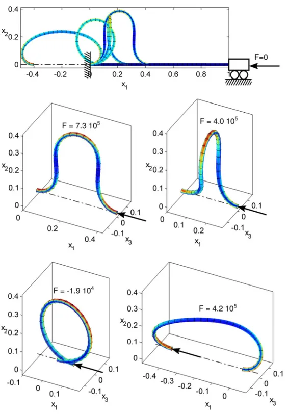
![Fig. 12. Deformed shape of the initially curved rod for the Lazarus et al. [21] experiment.](https://thumb-eu.123doks.com/thumbv2/123doknet/7416789.218712/15.892.483.809.706.1075/fig-deformed-shape-initially-curved-rod-lazarus-experiment.webp)
![Fig. 13. Equilibrium curve of straight (left) and curved (right) Lazarus et al. [21] rods.](https://thumb-eu.123doks.com/thumbv2/123doknet/7416789.218712/16.892.169.728.82.310/fig-equilibrium-curve-straight-left-curved-right-lazarus.webp)
![Daniel Glattauer - "Quand souffle le vent du Nord" [Critique]](data:image/gif;base64,R0lGODlhAQABAIAAAP///wAAACH5BAEAAAAALAAAAAABAAEAAAICRAEAOw==)