Université de Montréal
The Berth Allocation Problem at Port Terminals: A Column Generation Framework
par
Yousra Saadaoui
Département d’informatique et de recherche opérationnelle Faculté des arts et des sciences
Mémoire présenté à la Faculté des études supérieures en vue de l’obtention du grade de Maître ès sciences (M.Sc.)
en Informatique
juillet, 2015
c
The berth allocation problem (BAP) is one of the key decision problems at port termi-nals and it has been widely studied. In previous research, the BAP has been formulated as a generalized set partitioning problem (GSPP) and solved using standard solver. The assignments (columns) were generated a priori in a static manner and provided as an input to the optimization model. The GSPP approach is able to solve to optimality rela-tively large size problems. However, a main drawback of this approach is the explosion in the number of feasible assignments of vessels with increase in problem size which leads in turn to the optimization solver to run out of memory.
In this research, we address the limitation of the GSPP approach and present a col-umn generation framework where assignments are generated dynamically to solve large problem instances of the berth allocation problem at port terminals. We propose a col-umn generation based algorithm to address the problem that can be easily adapted to solve any variant of the BAP based on different spatial and temporal attributes. We test and validate the proposed approach on a discrete berth allocation model with dynamic vessel arrivals and berth dependent handling times. Computational experiments on a set of artificial instances indicate that the proposed methodology can solve even very large problem sizes to optimality or near optimality in computational time of only a few minutes.
pro-iii gramming, set partitioning, column generation.
Le problème d’allocation de postes d’amarrage (PAPA) est l’un des principaux prob-lèmes de décision aux terminaux portuaires qui a été largement étudié. Dans des recherches antérieures, le PAPA a été reformulé comme étant un problème de partitionnement généralisé (PPG) et résolu en utilisant un solveur standard. Les affectations (colonnes) ont été générées a priori de manière statique et fournies comme entrée au modèle Cette méthode est capable de fournir une solution optimale au problème pour des instances de tailles moyennes. Cependant, son inconvénient principal est l’explosion du nom-bre d’affectations avec l’augmentation de la taille du problème, qui fait en sorte que le solveur d’optimisation se trouve à court de mémoire.
Dans ce mémoire, nous nous intéressons aux limites de la reformulation PPG. Nous présentons un cadre de génération de colonnes où les affectations sont générées de manière dynamique pour résoudre les grandes instances du PAPA. Nous proposons un al-gorithme de génération de colonnes qui peut être facilement adapté pour résoudre toutes les variantes du PAPA en se basant sur différents attributs spatiaux et temporels. Nous avons testé notre méthode sur un modèle d’allocation dans lequel les postes d’amarrage sont considérés discrets, l’arrivée des navires est dynamique et finalement les temps de manutention dépendent des postes d’amarrage où les bateaux vont être amarrés. Les résultats expérimentaux des tests sur un ensemble d’instances artificielles indiquent que la méthode proposée permet de fournir une solution optimale ou proche de l’optimalité
v même pour des problème de très grandes tailles en seulement quelques minutes.
Mots clés: ordonnancement, allocation de postes d’amarrage, terminaux por-tuaires, programmation en nombres entiers mixtes, partitionnement, génération de colonnes.
Abstract . . . ii
Résumé . . . iv
Contents . . . vi
List of Tables . . . viii
List of Figures . . . ix
Acknowledgments . . . x
Chapter 1: Introduction . . . 1
1.1 Thesis motivation and objectives . . . 1
1.2 Thesis contribution . . . 5
1.3 Thesis outline . . . 6
Chapter 2: Literature Review . . . 7
2.1 Formulations . . . 7
2.1.1 Static BAP . . . 8
2.1.2 Dynamic BAP . . . 9
2.1.3 BAP in integration with other problems . . . 13
vii 2.2.1 Exact methods . . . 15 2.2.2 Heuristic approaches . . . 17 2.2.3 Summary . . . 21 Chapter 3: Methodology . . . 23 3.1 Problem definition . . . 23 3.2 MIP formulation . . . 24 3.3 GSPP formulation . . . 27 3.4 Column generation . . . 31
Chapter 4: Numerical Results . . . 39
4.1 Generation of instances . . . 39
4.2 Results and analysis . . . 42
Chapter 5: Conclusions and Future Work . . . 50
3.1 Input data for vessels . . . 28
3.2 Input data for berth sections . . . 28
3.3 Assignment matrix for a simple example of GSPP . . . 29
4.1 Berthing layout for |M| = 10 . . . 40
4.2 Description of instance classes A, B, C, D, E and F . . . 41
4.3 Description of instance class G . . . 42
4.4 Computational comparison between the algorithms for instances A, B, C and D . . . 47
4.5 Computational comparison between the algorithms for instances E, F and G . . . 48
4.6 Results obtained from the CG with the improvement technique for congested instances E, F and G . . . 49
List of Figures
1.1 Discrete berth layout . . . 3
1.2 Continuous berth layout . . . 3
1.3 Hybrid berth layout . . . 4
1.4 Feasible BAP Solution . . . 5
3.1 The dynamic column generation scheme for the BAP . . . 37
I would like to extend my deepest gratitude to my advisor, Dr. Emma Frejinger. It has been an honour and privilege to work under her supervision. I have the deepest respect for Dr. Nitish Umang for his guidance and support throughout the completion of this thesis. This work would not have been possible without his ability to stimulate imagination and creativity.
I am grateful to the committee members Dr. Bernard Gendron and Dr. Jean-Yves Potvin, for their critical review and constructive suggestions.
Chapter 1
Introduction
1.1
Thesis motivation and objectives
Port terminals are an important part of the global transportation of containers. Within a container terminal, there are three areas: the berth where vessels are docked for service, the stowage yard area where containers are stored temporarily waiting to be exported or imported, and the land-side area where trucks and trains are serviced. Accordingly, oper-ations in a container terminal can be broken down into two categories: seaside operoper-ations and land-side operations. To maintain competitive edge, the port managers must provide the best services. One way to do so is to improve port-operations efficiency and produc-tivity. In other words, they are obliged to use efficiently resources such as berths, cranes and yard equipment in order to optimize costs and customer satisfaction. Berths are con-sidered the most important resource and the berth allocation problem constitutes one of many complex seaside planning-and-operations problems container ports encounter.
Given a berth layout of a container terminal and a set of vessels, the berth allocation problem (BAP) refers to the problem of assigning berth positions and berthing times to incoming vessels that have to be unloaded and/or loaded in a given planning horizon such that some objective function is optimized. There are several important constraints
that need to be considered, for example, the depth of the berth must be higher than the vessel draft, the length of the vessel cannot exceed berth length and so forth. One of the most used objective functions is the minimization of the sum of the waiting and service times of each vessel. Other objective functions are minimization of number of rejected vessels, minimization of deviation between actual and planned berthing schedules, etc.
A variety of optimization models for the BAP have been proposed in the literature to capture real features of practical problems. The BAP can be considered static, dynamic or cyclic. In the static case, we assume that all vessels have arrived at the port and wait for being served. Hence, there are no arrival times given for the vessels and they can berth at any time given that the assigned quay portion is available for berthing. In the dynamic variant of the problem, the vessel arrive at individual and fixed arrival time is given for each one. So, the vessels cannot berth before the expected arrival times. In the cyclic arrivals, the vessels call at terminals repeatedly in fixed time intervals according to their liner schedule. The arrival times of vessel can be deterministic parameters or stochastic parameters defined by a discrete or continuous random distribution. In some papers, a due date for the vessel departure or a maximum waiting time for a vessel before the berthing time is predefined.
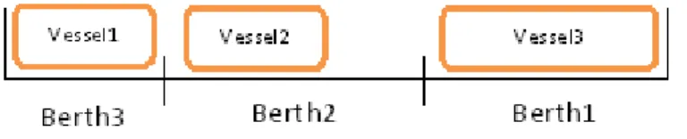
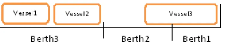
The BAP can also be modeled as a discrete,continuous or hybrid problem. The prob-lem is discrete if the quay is divided into berths, and a given berth can be used by only one vessel at a time. In the continuous case, the quay is not partitioned and a vessel can be moored in any arbitrary position along the quay. In the hybrid case, the quay
3 is divided into a set of berths, but two vessels or more may share the same berth at the same time, and a vessel may occupy more than one berth at a given time. A graphical representation of different berth layouts is shown in Figures 1.1, 1.2 and 1.3. Not only berth layout, but also draft restrictions may be considered when the feasible berthing positions of vessels are limited to only those berths that have a draft higher than the draft of the vessel.
The handling time may be assumed fixed and unchangeable, dependent on berthing position, dependent on the assignment of quay cranes or dependent on the quay crane operation scheduling. In addition, it may be stochastic to take into account uncertainty due to incidents such as equipment breakdown.
Figure 1.1: Discrete berth layout
Figure 1.2: Continuous berth layout
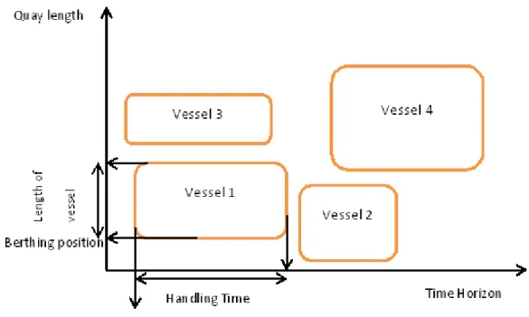
Figure 1.4 represents a feasible BAP solution including berthing positions and berthing times. The vertical axis corresponds to the quay space within the quay boundary, while the horizontal axis corresponds to berthing time within the planning horizon. Each
rect-Figure 1.3: Hybrid berth layout
angle is a vessel moored at the port. The length of the vessel is represented by the height of the rectangle; the berthing position along the quay is indicated by the upper and lower coordinates. The handling time of the vessel is represented by the width of the rectangle, the start and end of handling time are indicated by the left and the right coordinates, respectively. Overlapping in both time and space simultaneously is not permitted and infeasible while two vessels or more may be overlapping in space or time. Thus, as shown in Figure 1.4, all rectangles are non-overlapping. Due to this representation of the BAP on the time space graph, the berth allocation problem may be modeled as a 2-D bin packing problem (Lim (1998)).
In the operations research literature on port operation planning, there are several stud-ies on the different variants of the BAP and various formulations have been proposed. While most of these studies have focused on heuristic approaches in order to obtain good sub-optimal solutions to the BAP, a few recent studies propose exact methods to solve realistic sized instances of the BAP in reasonable computation time. The research pre-sented in this thesis focuses on exact methods to solve large problem instances of BAP to optimality.
5
Figure 1.4: Feasible BAP Solution
1.2
Thesis contribution
Among the exact methods proposed in the past to solve the BAP, the set partitioning (SP) approach is able to solve to optimality small size instances, but it has some short-comings and limitations in solving large problem instances. In such cases, the method can be very slow or can cause the optimization solver to run out of memory owing to an explosion in the number of variables and constraints in the SP formulation. The main contribution of this thesis is to propose a dynamic column generation scheme that is capable of solving very large problem size to optimality or near optimality in small computation time. Moreover, the approach can be used to solve any variant of the BAP with respect to the berthing layout or any other attribute(s).
1.3
Thesis outline
The remainder of the thesis is organized as follows. The next chapter provides a literature review of the existing models and formulations of the BAP as well as exact and heuristic approaches developed to solve it. In chapter 3, we present models to solve the discrete dynamic variant of BAP: a MIP formulation, a generalized set partitioning problem (GSPP) method, and a dynamic column generation framework. Results and analysis from computational experiments on a set of artificial instances are presented in Chapter 4. In the last chapter, the key findings of the study are summarized and some possible directions for future research are discussed.
Chapter 2
Literature Review
This chapter presents a comparative and analytical review of the existing research ef-forts relating to BAP. Existing models and formulations are reviewed in the first section based on their efficiency in addressing key operational and tactical questions relating to vessel service, and relevance and applicability to different berth planning. The advan-tages and limitations of most relevant exact and heuristic approaches developed to solve the BAP are discussed in the second section.
2.1
Formulations
Different mathematical models have been designed and several exact approaches and heuristic procedures have been proposed for the BAP. Steenken et al. (2004), Stahlbock and Voss (2008), Bierwirth and Meisel (2010) and recently Bierwirth and Meisel (2015) provide a detailed review of models and solution approaches for the planning of berth allocation.
The first studies dealing with the BAP problem, such as Nikolaou (1967), Sabria and Daganzo (1989) and other researches, focused on queuing theory using different repre-sentations of the problem. This approach failed to capture several of the attributes of the problem. Hence, and since 1990, research in the BAP has only focused on mathematical
programming and simulation.
2.1.1
Static BAP
Imai et al. (1997) were the first ones to study the static variant of the discrete BAP without considering the First Come First Served (FCFS) basis. The problem is formu-lated as a two objective non-linear integer program. The first objective minimizes the staying (waiting and handling) times of vessels, while the second minimizes the dissat-isfaction of the berthing order which refers to the deviation between the arrival order of vessels and their service order. The problem is reduced into a single objective problem consisting of the summation of the staying times and dissatisfaction.
Li et al. (1998) formulated the static BAP with fixed vessel handling time as a scheduling problem with a single processor through which multiple jobs can be pro-cessed simultaneously with the objective to minimize the makespan. The authors con-sidered the fixed position case and the non-fixed position case and stated that both cases could be applicable to the BAP under different assumptions (infinite and negligible ves-sel setup time and cost for job interruption/position change after the job has started). Guan et al. (2002) deal with the BAP and considered it as a multiprocessor task schedul-ing where a vessel (job) is assigned to a number of cranes (processors). In this paper, the authors assigned weights to each vessel in terms of its size and proposed to minimize the total weighted completion time of vessel service. Two cases of weights are considered but no priority service rules are employed.
9 Lim (1998) is the first to consider the continuous dynamic BAP. The problem was formulated as a graph with directed and undirected edges and transformed into a re-stricted version of the two-dimensional packing problem. His objective was to minimize the maximum amount of quay space used at any time with the assumption that the vessel will not be moved to any place along the quay once it is berthed. He also assumed that every vessel is berthed as soon as it arrives at the port.
Guan and Cheung (2004) proposed two mathematical models for the continuous berth allocation problem. The first one is the Relative Position formulation. It is com-parable to the model presented in Nishimura et al. (2001), but it is quite different in the objective which is to minimize the total weighted flow time. This formulation is used to develop a tree-search procedure in order to find the optimal solution of the problem. The second model is the Position Assignment formulation which is used to calculate a tight lower bound that can speed up the tree-search procedure.
2.1.2
Dynamic BAP
Imai et al. (2001) extended the static variant of the discrete BAP presented by Imai et al. (1997) to a dynamic variant. In their study, the water depth was assumed to be the same for all berths. They assumed also that the handling time is deterministic and depen-dent on the berth. The objective was to minimize the sum of vessels waiting and handling times. Hansen and Oguz (2003) criticized the model formulation by Imai et al. (2001) and proposed a more compact MIP formulation. Nishimura et al. (2001) addressed the
same problem, but with multi-water depth configuration in public berth system with number of berths. The berth allocation in this system, i. e.,the assignment of berths to incoming vessels for their cargo handling, plays an important role in minimizing the turnaround time. They assume that each berth can service multiple vessels as long as the berth length is not less than the total length of the vessels. Monaco and Sammarra (2007), inspired by the discrete and dynamic BAP of Imai et al. (2001), proposed an improvement in their formulation using fewer variables and constraints. It is shown to be stronger than the previous one.
Imai et al. (2003) extended the dynamic formulation of Imai et al. (2001) and Nishimura et al. (2001). They modified the existing BAP formulation in order to take into account service priority with respect to minimum waiting and handling times of the vessels. Un-like Nishimura et al. (2001), they dropped spatial restrictions (water depth and quay length) and assumed that only one vessel can occupy a berth at a given time. The vessel handling time is assumed dependent on the berth where it is assigned.
Kim and Moon (2003) investigate the continuous dynamic BAP with fixed handling time and present a mixed-integer-programming (MIP) model to minimize delays and handling cost. Unlike Imai et al. (2001), a cost penalty is applied to berthing in non-preferred berths. Priority service rule inclusion was not stated explicitly, though the objective function includes a penalty for the late departure of each vessel.
Dai et al. (2004) formulate the static and dynamic versions of the continuous BAP as a rectangle packing problem with release time constraints. More precisely, they model
11 the associated BAP as a problem of packing rectangles in a semi-infinite strip with gen-eral spatial cost structure. The objective is to minimize the delays faced by the vessels, with higher priority vessels receiving promised level of services, while at the same time addressing the desirability to berth the vessels on designated locations along the termi-nal minimizing the movement and exchange of containers within the yards and between vessels.
Imai et al. (2005) considered the discrete BAP first, and then extended their work by solving the dynamic BAP in a continuous berth space. The objective is the minimization of the total service and waiting times with deterministic handling times depending on berthing position (all the existing continuous BAP studies up to date assume that han-dling times are known in advance and cannot change). Chang et al. (2008) extended this model by including vessel draft constraints.
Similar to Imai et al. (2005), Cordeau et al. (2005) formulated the dynamic and dis-crete BAP as a multi-depot vehicle routing problem with time windows (MDVRPTW). Berths are represented as depots, while vessels are considered customers. The MD-VRPTW objective function is to minimize the total vessel service time. In contrast to previous models, their work is capable of handling a weighted sum of service times as well as windows on berthing times.
In Christensen and Holst (2008), an alternative approach has been presented; the BAP is formulated as a generalized set-partitioning problem (GSPP). Time is discretized and the assignment matrix is generated by data preprocessing, where a column (variable)
represents a feasible berthing assignment of a single vessel to a specific berth at a spe-cific time. Buhrkal et al. (2011) show that the GSPP model is able to significantly out-perform the model presented in Imai et al. (2001) and the MDVRPTW model presented in Cordeau et al. (2005).
In a pioneering work on the berth template problem (BTP), Moorthy and Teo (2006) presented a new approach for the dynamic hybrid BAP with fixed handling times and stochastic vessel arrivals. As defined by Imai et al. (2014), the berth template problem (or tactical berth scheduling) finds a set of berth-windows (i.e., berthing locations with start and end times for service) within the fixed length of planning horizon so as to maximize the service objective. Moorthy and Teo (2006) model this as a rectangle packing problem on a cylinder as the fixed planning horizon is repeated in a cyclic fashion. The problem is formulated as a bi-criteria optimization problem in order to define berthing positions of vessels at a tactical level. The first objective is the service level-waiting time. It deals with stochasticity in the arrival of vessels and robustness of the final schedule. The second objective is the operational cost-connectivity. It deals with the trade-off between the operational cost of moving containers from one vessel to the other and the delays (difference between actual arrival time at the port and start time of berthing). Authors state that their approach is limited by the fact that the template is relevant only when a substantial number of vessels arrive periodically and within the same period.
13
2.1.3
BAP in integration with other problems
A very interesting extension of the BAP is to combine the BAP with Quay Crane (QC) Assignment, which was introduced by Park and Kim (2003). The model presented aims at determining the vessel berthing times, the associated berthing positions and si-multaneously the optimal assignment of quay cranes to vessels. So, the objective func-tion is more elaborate than the ones by Park and Kim (2002) as there are different cost penalties namely: handling cost, delay, early arrival and late arrival. In this study, the au-thors assumed that the crane productivity is proportional to the number of QCs, despite the fact that quay crane interference reduces the marginal productivity. In the same con-text, Imai et al. (2008) consider the crane resource within a discrete BAP, but do not take into account the relationship between the number of quay cranes and handling time. It is assumed that a certain number of QCs has to be assigned to each vessel. In the approach of Meisel and Bierwirth (2009), the crane productivity depends on the berthing position of vessels and the crane productivity losses by interference are modeled. However, like the previous studies, this paper assign quay cranes hour by hour without controlling the final outcome. The model proposed by Giallombardo et al. (2010) and later used by Vacca et al. (2013) addresses the unrealistic assumptions of the early stated models. The authors deal with the berth allocation problem at the tactical level. They assume that quay cranes can be moved from one vessel to another only at the end of the working shift and take into account in the profile definition the productivity losses due to inter-ference. Furthermore, the handling time directly associated with the vessel depends on
the number of assigned quay cranes. Giallombardo et al. (2010) present two mixed in-teger programming formulations. The objective is to maximize the difference between the revenue associated with the chosen quay cranes profile and the housekeeping costs generated by transshipment flows among the vessels. A quay crane profile is defined by its monetary value, i.e., the price charged by the terminal to the shipping companies for the provided service, its time duration, and the number of quay cranes by shift.
Hendriks et al. (2010) address the integrated planning of berth allocation and quay crane assignment to meet service agreements contracted between ports and vessel op-erators at minimum crane capacity. This paper considers cycle arrivals of vessels, and develops a berth template of fixed length that serves as a blueprint over a long time pe-riod. The berth template is modeled as a packing problem on a cylinder to insure that the service of those vessels that are scheduled to the end of the planning horizon extend into the subsequent planning period. Hendriks et al. (2012) extend the berth template problem to multi-terminal ports where vessels can berth at any terminal in a port with inter-terminal service agreements. This study assumed cyclically calling vessels, hence we can say that the cylinder model is implicitly imposed.
2.2
Solution methods
The different models proposed for the various variants of the BAP are very complex given that the BAP has been shown to be NP-hard, see e.g, Hansen and Oguz (2003), and Lim (1998). Therefore, heuristic approaches are mostly used to solve the problem. In
15 fact, only few papers proposed exact methods such as branch-and price, branch-and-cut or standard solvers (CPLEX, Lindo, etc...) with mixed integer linear programming for-mulations. In contrast, several heuristic and meta-heuristic approaches were developed like genetic algorithms, tabu search, etc.
2.2.1
Exact methods
Buhrkal et al. (2011) are the first to attempt to solve exactly the berth allocation problem. They have compared different models for the dynamic discrete variant of the BAP. For the comparison, they considered five instances size and used a CPLEX solver. They stated that the GSPP formulation proposed by Christensen and Holst (2008) out-performs the reformulation of Monaco and Sammarra (2007) of the model formulated in Imai et al. (2001) and the MDVRPTW model proposed in Cordeau et al. (2005). The performance of the GSPP is quite remarkable. For all the instances containing up to 60 vessels, the model is able to find the optimal solution in computational time less than 30 seconds. In the same context, Umang et al. (2013) confirm the findings of Buhrkal et al. (2011). They demonstrate the superiority of the SP approach, where the planning hori-zon is partitioned into time buckets of 1 hours, by comparing three different formulations of the dynamic BAP with a hybrid berthing layout in the context of bulk port terminals. The approach can solve to optimality instances up to 40 vessels within a computational time limit of 2 hours. However, for some instances with 40 vessels, CPLEX runs out of memory. To fix this issue, the planning horizon is partitioned into larger time buckets of
2 hours. A few other authors propose exact algorithms to solve the BAP in integration with other optimization problems. For example, Vacca et al. (2013) propose a model for the integrated berth allocation and quay crane assignment problem in port container terminals, and implement an exact branch-and-price algorithm, proving good quality bounds and optimal solutions to the problem. The algorithm is based on Dantzig-Wolfe decomposition of the original MIP formulation defined by Giallombardo et al. (2010) for the tactical berth allocation problem. The maximum problem size in this study contains 20 vessels and 5 berths over a planning horizon of one week. Computational results reveal that the proposed algorithm outperforms commercial solvers. Turkogullari et al. (2013) did likewise and proposed an exact algorithm to solve the berth allocation quay crane assignment and scheduling problem (BACASP). They designed and implemented a cutting plane algorithm to derive an optimal solution for the BACASP from the opti-mal solution of the berth allocation and quay crane assignment problem (BACAP). The developed algorithm is able to solve large instances containing up to 60 vessels in a few hours. In a recent paper, Robenek et al. (2014) propose an exact solution algorithm based on a branch and price framework to solve the dynamic hybrid BAP in integration with the yard assignment problem in bulk terminals. The authors reformulate the integrated model as a set partitioning problem and a column generation approach is applied. Re-sults show that instances containing up to 40 vessels can be solved within reasonable computational times of a few hours.
17
2.2.2
Heuristic approaches
In order to solve the BAP, most researchers have developed heuristics and meta-heuristics. Even though we focus on exact methods in this thesis, we present some of these methods in the following.
2.2.2.1
Genetic algorithm
The genetic algorithm (GA) is a search heuristic that mimics the process of natural selection. This heuristic is routinely used to generate useful solutions to optimization and search problems. The GA was proposed for different models and variants of the BAP. Nishimura et al. (2001) presented a genetic algorithm to solve a discrete space and dynamic BAP. The proposed GA was compared against results from a Lagrangian relaxation heuristic, with the latter performing slightly better but without significant dif-ferences.
Han et al. (2006) studied the discrete dynamic BAP and presented a hybrid optimiza-tion strategy based on a combinaoptimiza-tion of GA and Simulated Annealing (SA). The authors kept the same GA characteristics as those used in Nishimura et al. (2001). To select the individuals of the next generation, they applied a stochastic process using param-eters given by the SA approach. Compared to results obtained from the GA heuristic without the stochastic component, the proposed heuristic performs better. Theofanis et al. (2007) were the first to present an optimization based GA heuristic for the discrete dynamic BAP. The authors applied the GA based heuristic proposed by Golias et al.
(2007) and followed the same representation as Nishimura et al. (2001). They used four different types of mutation but no crossover. Similar to the research presented so far, the proposed heuristic was only compared to the GA heuristic without the optimization component (an internal optimization heuristic embedded right after the genetic opera-tions are completed and before the next generation selection). Results showed that the former outperformed the latter. The increase in computational time due to the optimiza-tion component was negligible. The proposed algorithm could be applied to any linear formulation of the BAP. Golias et al. (2009) developed a GA based heuristic to solve the discrete and dynamic BAP formulated as a multi-objective combinatorial optimization problem. Results showed that the proposed algorithm outperformed a state-of-the-art meta-heuristic and provided improved results when compared to the weighted approach. Imai et al. (2008) introduced a GA based heuristic to find an approximate solution to the berth scheduling problem without consideration of the quay cranes. The QC assign-ment was performed by solving a maximum flow problem. The proposed GA heuristic was very interesting as the chromosomes only produced the vessel-to-berth service or-der and before reproduction, crane scheduling was performed. A two-point crossover was used for reproduction, and selection was based on the fitness function presented in Nishimura et al. (2001). Based on trend analysis of the numerical results, the au-thors concluded that the proposed heuristic is able to solve the problem. In Rodriguez-Molins et al. (2014) a mixed integer programming (MIP) model and a new hybrid multi-objective genetic algorithm were developed for the dynamic and continuous
ro-19 bust BAP and QC assignment problem. The results showed that the MIP model and the multi-objective GA were able to obtain robust and efficient schedules up to 10 incoming vessels.
2.2.2.2
Simulated annealing
Simulated Annealing (SA) is a probabilistic method proposed for finding the global minimum of a cost function that may possess several local minima. For certain problems, simulated annealing may be more efficient than exhaustive enumeration, provided that the goal is merely to find an acceptably good solution in a fixed amount of time. Kim and Moon (2003) used SA to find near optimal solution for the continuous dynamic BAP. They compared their heuristic to classic optimization techniques and found that the SA algorithm resulted in near optimal solution and that the computational time was within the limits of practical usage. Recently, Lin and Ting (2014) proposed SA approaches to solve two versions of the dynamic berth allocation problem: discrete and continuous. The proposed SAs are tested with numerical instances from the literature. Experimental results show that SA can obtain the optimal solutions for all instances in discrete case and 27 best known solutions in the continuous case. In De-Oliveira et al. (2012a), the BAP is considered as dynamic and discrete. A new alternative based on applying the Clustering Search (CS) method using SA for solution generation is proposed. The CS is an iterative method that divides the search space in clusters and it is composed of a meta-heuristic for solution generation, a grouping process and a local search heuristic.
2.2.2.3
Tabu search
Tabu search is a meta-heuristic employing local search methods. It uses a flexible structure memory, conditions for strategically constraining and freeing the search pro-cess, and memory function of varying time span for intensifying and diversifying the search. Cordeau et al. (2005) proposed a tabu search to solve the dynamic berth al-location problem in the discrete case by considering this problem as a variant of the MDVRPTW. This heuristic is called T2S(Time based Tabu Search), since it focuses on the temporal dimension. An extension of the tabu search heuristic to the spatial dimen-sion is also presented for the continuous case. It is called (T S)2 (Time and Space based Tabu Search). Lalla-Ruiz et al. (2012) propose a hybrid heuristic that combines the tabu search meta-heuristic with path relinking (T2S+ PR) to solve the dynamic berth allo-cation problem. The proposed hybrid algorithm is compared with the T2Sproposed by Cordeau et al. (2005). Results indicate that the hybrid heuristic out performs T2S con-sidering both solution quality and computational times. Compared to the GSPP model presented by Christensen and Holst (2008), the T2S+ PR produces optimal or near opti-mal solution in a sopti-maller amount of time than GSPP. It can also solve medium and large size instances for which GSPP cannot be solved to optimality.
The heuristics mentioned above are the most relevant ones found in the literature, however other heuristic (or meta-heuristic) algorithms were developed. For example, the particle swarm approach (PSO) is used by Ting et al. (2014) to solve the discrete and dynamic BAP using two sets of benchmark instances from the literature. Results
21 show that the PSO algorithm is better than other recent algorithms for the BAP, namely Tabu Search (T2S) (Cordeau et al. (2005)), population training algorithm with linear programming (PTA/LP) (Mauri et al. (2008)), and the clustering search (CS) approach (De-Oliveira et al. (2012b)). Another meta-heuristic called Greedy Randomized Adap-tive Search Procedure (GRASP) was used by Salido et al. (2011) and Salido et al. (2012) for the combined BAP and quay crane assignment. Rodriguez-Molins, Salido and Barber (2014) also develop a GRASP based meta-heuristic for the same problem by managing vessel cargo holds.
Cheong et al. (2007) develop a Multi-Objective Multi-Colony Ant Algorithm (MOM-CAA) for solving the berth allocation problem in multi-user terminal, by exploiting an island model with heterogeneous colonies. Each colony may be different from the oth-ers in terms of the combination of pheromone matrix and visibility heuristic used. In contrast to conventional ant colony optimization (ACO) algorithms, where each ant in the colony searches for a single solution, the MOMCAA uses a group of ants to search for each candidate solution. Each ant in the group is responsible for the schedule of a particular berth in the solution.
2.2.3
Summary
From the literature review, we note that the SP formulation has been successfully used to solve the BAP in past studies ( Christensen and Holst (2008), Buhrkal et al. (2011), Umang et al. (2013)). The main drawback of this exact approach is that it cannot
solve large instances to optimality. We address this drawback by proposing a GSPP for-mulation and a column generation algorithm, where columns are generated dynamically, to solve large size instances of the BAP.
Chapter 3
Methodology
In order to test and validate the column generation approach, we use a dynamic dis-crete model with the objective to minimize the total service times of the vessels. In this chapter, we present a mixed integer programming (MIP) formulation and a GSPP model to solve realistic sized instances of the BAP, and propose a dynamic column generation based scheme to address the limitations of the GSPP approach.
3.1
Problem definition
In this study, we propose a column generation based approach that can be easily adapted to solve any variant of the BAP based on spatial attributes such as the berthing layout and draft restrictions, as well as temporal attributes such as vessel arrival times and handling times. To test and validate our approach, we consider a set of vessels N, to be berthed on M berth positions of variable lengths implying that a given vessel can occupy only one discrete berth section at a given time. We consider a dynamic vessel arrival process where some vessels may arrive after the planning start time and each vessel docks on a berth position after its expected arrival times. The planning horizon is considered to be fixed and partitioned into discrete time buckets. The handling time of a vessel is assumed to depend on the berthing location of the vessel along the quay.
3.2
MIP formulation
In this section, we present a more formal description for the Dynamic Discrete BAP and introduce a MIP formulation for the problem inspired from the model proposed by Kim and Moon (2003) for the continuous dynamic BAP. We first introduce the following notation:
N : set of vessels, |N| = n M : set of berths, |M| = m
hki : Handling time spent by vessel i ∈ N at berth k ∈ M ai : Arrival time of vessel i
li : Length of vessel i ∈ N
di : Draft of vessel i ∈ N Lk : Length of berth k ∈ M Dk : Depth of berth k ∈ M B : Large positive constant.
The MIP model has the following decision variables.
σijx=
1 if vessel i ∈ N is located to the left of vessel j ∈ N on the wharf; 0 otherwise. σijy=
1 if vessel i ∈ N is berthed before vessel j ∈ N in time; 0 otherwise.
25 xki =
1 if berth k ∈ M is assigned to vessel i ∈ N; 0 otherwise.
yi: ≥ 0, Berthing time of vessel i ∈ N.
The clearance distances between adjacent vessels as well as end-clearances may be considered implicitly in vessel lengths. Similarly, the clearance times between two suc-cessive vessels overlapping in space may be considered implicitly in the handling times. The MIP model for the dynamic berth allocation problem with discrete berth layout at port terminals is formulated as shown below.
min
∑
i∈N (yi− ai+∑
k∈M (hkixki)) (3.1) s.t.∑
k∈M xki = 1 ∀i ∈ N (3.2) yi− ai≥ 0 ∀i ∈ N (3.3)∑
k∈M (Dk− di) xki ≥ 0 ∀i ∈ N (3.4)∑
k∈M (Lk− li) xki ≥ 0 ∀i ∈ N (3.5) yj+ B(1 − σi jy) ≥ yi+∑
k∈M (hkixki) ∀i, j ∈ N, i 6= j (3.6)∑
k∈M (kxki) + B(1 − σi jx) ≥∑
k∈M (kxki) + 1 ∀i, j ∈ N, i 6= j (3.7) σi jx+ σxji+ σi jy+ σyji≥ 1 ∀i, j ∈ N, i 6= j (3.8) yi≥ 0 ∀i ∈ N (3.9) xki ∈ 0, 1 ∀i ∈ N, k ∈ M (3.10) σi jx, σi jy ∈ 0, 1 ∀i, j ∈ N, i 6= j (3.11)The objective function (3.1) minimizes the total service times (sum of delay and handling time) of all vessels berthing at the port. Constraints (3.2) ensure that every vessel must be serviced once at any berth. Constraints (3.3) ensure that each vessel is serviced after its arrival. Constraints (3.4) guarantee that the draft of any vessel does not exceed the draft of the occupied berth. Constraints (3.5) ensure that the length of any vessel does not exceed the length of the assigned berth. Constraint set (3.6)-(3.8) are the
27 non overlapping restrictions. Note that we linearized the two constraints (3.6) and (3.7) by using a large positive number B. Constraints (3.6) or (3.7) are effective only if σi jx or σi jy equals one and constraint (3.8) σi jx+ σxji+ σi jy + σyji= 0 in which case two vessels are in conflict with each other with respect to the berthing position.
Even though the above model is linear and small instances can be solved using com-mercially available solvers, computation time is long. Furthermore, it is not able to solve large instances (optimality gap values are large). Therefore, another formulation to solve the BAP is presented in the next section.
3.3
GSPP formulation
Christensen and Holst (2008) modeled the dynamic discrete BAP as a generalized set-partitioning problem (GSPP) in the context of container terminals. In their model, the planning horizon H is divided into discrete time intervals and all time measurements are integers. The assignment matrix is generated by data preprocessing, where a column (variable) represents a feasible berthing assignment of a single vessel to a specific berth at a specific time. Only those assignments where the vessel is occupying the berth and the estimated departure time of the vessel does not exceed the length of the planning horizon, are feasible. The first n rows correspond to the n vessels. If a column represents an assignment of vessel i, there will be a 1 in row i and zeros in the rest of the n first rows. Furthermore, there is one row for each available time unit at each berth. An entry in a column is equal to one if the vessel occupies the berth at the considered time unit,
otherwise it is zero. The cost of each column is equal to the service time arising from the vessel/berth/time assignment.
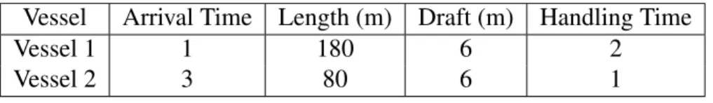
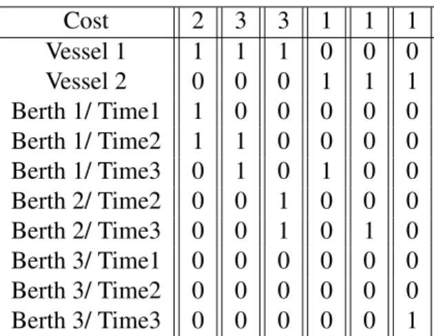
Table 3.3 represents the assignment matrix of a simple example of GSPP. This ex-ample has 3 berths and 3 discrete time intervals. Let us assume that berth number 1 is open from time 1-3, number 2 from 2-3 and number 3 from 1-3. We consider vessels 1 and 2 with handling time 2 and 1, respectively (on the 3 berths). Vessel number 2 arrives at the start of time 3, and hence can only berth after that. Input data for vessels and berth sections are presented in Tables 3.1 and 3.2 respectively. The first column represents the berthing assignment of vessel 1 to section 1 from time 1, and so on.
Vessel Arrival Time Length (m) Draft (m) Handling Time
Vessel 1 1 180 6 2
Vessel 2 3 80 6 1
Table 3.1: Input data for vessels
Berth Length (m) Draft (m)
Berth 1 250 8
Berth 2 190 8
Berth 3 100 8
Table 3.2: Input data for berth sections
Let S designate the set of columns. We define two matrices A and B, submatrix of the constraint matrix, both containing |S| columns. The first matrix A contains |N| rows, a row for each vessel. Ais = 1 if column s ∈ S represents a feasible assignment of
29 Cost 2 3 3 1 1 1 Vessel 1 1 1 1 0 0 0 Vessel 2 0 0 0 1 1 1 Berth 1/ Time1 1 0 0 0 0 0 Berth 1/ Time2 1 1 0 0 0 0 Berth 1/ Time3 0 1 0 1 0 0 Berth 2/ Time2 0 0 1 0 0 0 Berth 2/ Time3 0 0 1 0 1 0 Berth 3/ Time1 0 0 0 0 0 0 Berth 3/ Time2 0 0 0 0 0 0 Berth 3/ Time3 0 0 0 0 0 1
Table 3.3: Assignment matrix for a simple example of GSPP
vessel i ∈ N, otherwise, Ais= 0. The second matrix B contains a row per (Berth / Time)
position. We assume that all berths are available for the berth allocation planning from the beginning until the end of the time horizon H. The rows of B are indexed by the set H defined below. Therefore Bts = 1 if position t ∈ H is in the assignment that column s
represents.
We assume the following input data to be available for the GSPP model:
H = set of discrete time intervals in the planning horizon. S= set of feasible assignments.
t= 1,. . . ,|H| discrete time intervals in the planning horizon. s= 1,. . . ,|S| feasible assignments.
ds= delay associated with assignment s which denote the difference between the
berth time and the arrival time of the vessel. hs= handling time associated with assignment z.
The assignment matrix coefficients are defined as follows. Ais=
1 if assignment s represents a feasible assignment for vessel i; 0 otherwise. Bkts =
1 if berth k is occupied at time t in assignment s; 0 otherwise.
There is only a single decision variable in the GSPP model for selection of feasible assignments in the optimal solution which is defined as follows.
xs=
1 if assignment s is part of the optimal solution; 0 otherwise.
The GSPP model is formulated as shown below:
min
∑
s∈S (ds+ hs)xs (3.12) s.t.∑
s∈S (Aisxs) = 1 ∀i ∈ N (3.13)∑
s∈S (Bkts xs) ≤ 1 ∀k ∈ M, ∀t ∈ H (3.14) xs ∈ {0, 1} ∀s ∈ S (3.15)The objective function (3.12) minimizes the total service time of vessels berthing at the port. Constraints (3.13) ensure that each vessel must have exactly one feasible assignment in the optimal solution, while constraints (3.14) enforce the restriction that a given section at a given time can be occupied by at most one vessel. A major limitation of
31 the set partitioning approach is the explosion in the number of variables and constraints with increase in problem size. Thus, the method may be very slow and the solver can run out of memory when the number of feasible assignments is too large as determined by the problem size defined by the number of vessels and the number of berths along the quay, the length of the horizon time, the redundancy of one or more constraints such as the draft restrictions etc. In some cases, it is possible to make the method affordable at the risk of losing optimality by partitioning the planning horizon into fewer discrete time buckets of larger size. The root cause of this problem is that the assignments (columns) are generated a priori and fed as an input to the model. To address this shortcoming to the model, we propose to solve the problem through column generation (CG) as described in the following section.
3.4
Column generation
In this section, a different approach to solve the GSPP formulation (3.12)-(3.15) is presented. In this novel scheme, the feasible assignments (columns) are generated in a dynamic way, in order to reduce the computational load on the solver. We consider the linear programing (LP) relaxation of the set partitioning problem, in which the domain of xs is extended to [0, 1]. It is possible to solve this LP relaxation using a column
generation algorithm even with the large number of variables. In the dynamic scheme, the LP relaxation of the SP formulation is referred to as the restricted master problem (RMP) as shown below. Ω denotes the active pool of columns. It contains only a subset
of all possible feasible assignments to the problem instance. New variables are added to Ω until no variable can further improve the solution that results from only using the variables in Ω. min
∑
s∈S (ds+ hs)xs (3.16) s.t.∑
s∈S (Aisxs) = 1 ∀i ∈ N (3.17)∑
s∈S (Bkts xs) ≤ 1 ∀k ∈ M, ∀t ∈ H (3.18) xs ∈ [0, 1] ∀s ∈ Ω (3.19)In order to execute the column generation, we start with an initial feasible solution to the master problem obtained from a first come first served rule: vessels are sorted in ascending order of their arrival times. Then each vessel is sequentially assigned to the berth with the shortest handling time. If all berths are occupied, the berth with the earliest completion time is chosen. The algorithm designed to generate the initial feasible solution is described by Algorithm 1.
The initial solution comprising of |N|columns is added to Ω, so that in the first it-eration of column genit-eration, the RMP is solved using the set Ω containing |N| active columns. Subsequently, in each iteration of the column generation process, the values of the following dual variables are calculated and |N| sub-problems are solved, one for each
33 Algorithm 1 Heuristic to obtain an initial feasible solution for the dynamic CG
Require: Set N of vessels sorted by arrival times, set M of berths for i = 1 → N do
if BerthIsAvailable then
Assign vessel to berth with lowest handling time for vessel i end if
if BerthIsNotAvailable then
Assign vessel to berth with earliest completion time for vessel i end if
end for
vessel in the problem instances. The idea is to price out columns with negative reduced cost that can potentially improve the solution and add them to the active pool of active columns Ω. To this purpose, we introduce the following notation.
πithe dual variables corresponding to constraints (3.17)
τkt the dual variables corresponding to constraints (3.18)
We now describe the sub-problem formulation in detail. We note that the pricing sub-problem decomposes into one problem for each vessel, defined by the constraints corresponding to that vessel. So, in each iteration of column generation, we solve |N| sub-problems, one for each vessel i ∈ N. Each vessel sub-problem aims to identify the feasible assignment with the least reduced cost to be added to the current pool of active columns Ω in the RMP.
Note that since the sub-problem is solved separately for each vessel i ∈ N, the index iis dropped from all decision variables and parameters. The objective function minimiz-ing the reduced cost in each sub-problem can be written as:
min(y − a +
∑
k∈M
hkxk− π −
∑
t∈Hk∈M
∑
τktσkt) (3.20)
The following input data are used in the sub problem:
π , τkt : the dual variables obtained from the restricted master problem
a : the arrival time of the vessel l : the length of the vessel d : the draft of the vessel Lk : length of berth k Dk : draft of berth k
hk : handling time at berth k B : large positive constant
The decision variables used in the sub-problem are:
y integer ≥ 0, the starting time of handling the vessel
xk=
1 if berth k is occupied by the vessel; 0 otherwise. θt=
1 if the vessel is served at time t; 0 otherwise.
35 σkt=
1 if berth k is occupied at time t; 0 otherwise.
The sub-problem can be formulated as a mixed integer linear program as follows:
min(y − a +
∑
k∈M (hkxk) − π −∑
t∈Hk∈M∑
(τktσkt)) (3.21) y− a ≥ 0 (3.22)∑
k∈M (Lk− l)xk≥ 0 (3.23)∑
k∈M (Dk− d)xk≥ 0 (3.24)∑
k∈M xk= 1 (3.25)∑
t∈H θt =∑
k∈M (hkxk) (3.26) t+ B(1 − θt) ≥ y ∀t ∈ H (3.27) t≤ y +∑
k∈M (hkxk) + B(1 − θt) − 1 ∀t ∈ H (3.28) σkt≥ xk+ θt− 1 ∀t ∈ H, ∀k ∈ M (3.29) σkt≤ xk ∀t ∈ H, ∀k ∈ M (3.30) σkt≤ θt ∀t ∈ H, ∀k ∈ M (3.31) xk∈ {0, 1} ∀k ∈ M (3.32) θt∈ {0, 1} ∀t ∈ H (3.33) σkt∈ {0, 1} ∀k ∈ M, ∀t ∈ H (3.34)Constraint (3.22) ensures that the vessel should be served after its arrival. Constraint (3.23) ensures that the length of the vessel does not exceed the length of the assigned berth. Constraint (3.24) guarantees that the draft of the vessel does not exceed the depth of the occupied berth. Constraint (3.25) ensures that the vessel is assigned once at any berth. Constraints (3.26)-(3.28) control the values of the binary decision variables θt
ensuring they take a value equal to 1 at all times when the vessel is berthed. Constraints (3.29)-(3.31) control the values of the binary decision variables σkt to ensure that they take a value equal to 1 if and only if both xkand θtare equal to 1.
The decomposition of the sub-problem into |N| sub-problems reduces its complex-ity. Thereby, the sub-problem (3.21)-(3.34) can be easily solved using polynomial time heuristic or directly using an optimization solver such as CPLEX. The |N| columns that are priced out in each iteration of the column generation, one for each vessel, and have negative reduced cost, are added to the active pool of columns Ω, and the RMP (3.16)-(3.19) is re-solved. The dual variable values are obtained, the |N| subproblems are solved and the process is continued iteratively until there are no negative reduced cost columns for any vessel. The main steps in the proposed column generation algorithm are shown schematically in figure 3.1 below.
Obtaining an integer solution
The solution of the LP relaxation RMP obtained after the convergence of the column generation algorithm is typically fractional, and is a lower bound to the original problem.
37
Figure 3.1: The dynamic column generation scheme for the BAP
In order to obtain an integer solution, we simply use an approach that works extremely well for the problem studied in this research. Once the column generation terminates, the integrality constraints (3.15) are reinforced and the problem is re-solved using the active pool of columns Ω at the end of the column generation process. The integer solution obtained is a valid upper bound to the problem we are interested in solving. If the gap between the upper bound and the lower bound is zero, then the upper bound is
also the optimal solution. If the gap is non-zero, the optimal solution can be determined through a branch-and-bound (B&B) algorithm (for more details on branch and bound, please refer to Hillier et al. (2001)), where column generation needs to be applied at each node of the B&B tree. The combination of column generation and B&B is called branch-and-price (see e.g. Vacca et al. (2013) and Robenek et al. (2014)).
Improvement Methods
In order to speed up the rate of convergence of the column generation process, the first strategy we considered was to retrieve more than one negative reduced cost columns per iteration per sub problem. We used a CPLEX function to access the solution pool. We applied this improvement method only for instances where the column generation method did not reach optimality. We conducted two sets of experiments in which we retrieved 5 and 10 negative reduced cost columns per iteration per sub problem.
Chapter 4
Numerical Results
The BAP models presented earlier in this study are compared in this chapter. We tested the MILP formulation described in (3.1)-(3.11) using CPLEX with the solution time limit set to 1800 seconds. All feasible berthing assignments for each instance are provided as an input to the GSPP model described in (3.12)-(3.15). The model is then solved using CPLEX solver. All tests were run on an Intel(R) Core(TM) i7 -3770 CPU(3.40 GHz) processor and used a 32-bit version of CPLEX 12.6. We used Java Programming language to implement the three algorithms.
4.1
Generation of instances
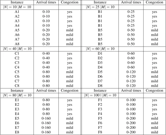
To test and compare the solution performance of the three algorithms, we generated 7 instance sizes with |N| = 10, 25, 40, 60, 80, 100 and 120 vessels and |M| = 10 berths. Even though we keep the number of berths fixed, these instances cover the character-istics that we which to test. A set of 8 instances was generated for each instance size. The arrival times ai are randomly generated between the range of values 0 and |N| for
congested instances and between 0 and 2 * |N| for mildly congested instances. Among the 8 generated instances, 4 are congested and the 4 others are mildly congested. Arrival times values are described in more detail later in the chapter.
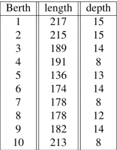
In all test instances, the vessel lengths lie in the range of 80 to 200 meters while vessel drafts vary between 6 and 12 meters. The number of berths is assumed to be 10 with berth lengths varying from 120 to 220 meters and berth draft between 8 and 15 meters. we note that we used the data in the literature to get a rough estimate of the range of values for most input parameters in our model. The berthing layout used in the instances is shown in Table 4.1.
Berth length depth
1 217 15 2 215 15 3 189 14 4 191 8 5 136 13 6 174 14 7 178 8 8 178 12 9 182 14 10 213 8
Table 4.1: Berthing layout for |M| = 10
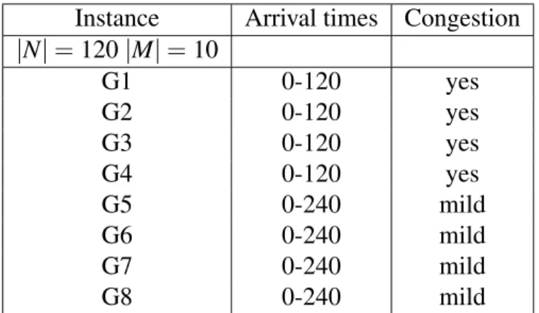
To test the sensitivity of the results with respect to the size of the instance and the level of congestion in the model, the instances have been designed as illustrated in Ta-bles4.2 and 4.3.
In all the generated instances, the handling times are drawn from a uniform distri-bution in the range of 6 to 20 hours. Since the handling time of a vessel depends on its berthing position, we generated, for each vessel, a handling time value for each berth.
41
Instance Arrival times Congestion Instance Arrival times Congestion |N| = 10 |M = 10 |N| = 25 |M| = 10 A1 0-10 yes B1 0-25 yes A2 0-10 yes B1 0-25 yes A3 0-10 yes B1 0-25 yes A4 0-10 yes B1 0-25 yes A5 0-20 mild B5 0-50 mild A6 0-20 mild B5 0-50 mild A7 0-20 mild B5 0-50 mild A8 0-20 mild B5 0-50 mild |N| = 40 |M| = 10 |N| = 60 |M| = 10 C1 0-40 yes D1 0-60 yes C2 0-40 yes D2 0-60 yes C3 0-40 yes D3 0-60 yes C4 0-40 yes D4 0-60 yes C5 0-80 mild D5 0-120 mild C6 0-80 mild D6 0-120 mild C7 0-80 mild D7 0-120 mild C8 0-80 mild D8 0-120 mild Instance Arrival times Congestion Instance Arrival times Congestion |N| = 80 |M| = 10 |N| = 100 | |M| = 10 E1 0-80 yes F1 0-100 yes E2 0-80 yes F2 0-100 yes E3 0-80 yes F3 0-100 yes E4 0-80 yes F4 0-100 yes E5 0-160 mild F5 0-200 mild E6 0-160 mild F6 0-200 mild E7 0-160 mild F7 0-200 mild E8 0-160 mild F8 0-200 mild
Instance Arrival times Congestion |N| = 120 |M| = 10 G1 0-120 yes G2 0-120 yes G3 0-120 yes G4 0-120 yes G5 0-240 mild G6 0-240 mild G7 0-240 mild G8 0-240 mild
Table 4.3: Description of instance class G
4.2
Results and analysis
The results from the computation experiments are shown in Tables 4.4 and 4.5. For |N| = 10 and 25 vessels, the MIP formulation can solve to optimality all instances within the prescribed CPLEX time limit of 30 minutes. However, for instances with |N| = 40, 60 and 80 it returns optimal solution only for mildly congested instances and is not able to solve even a single instance to optimality for |N| = 100 and 120 with a large duality gap (more than 20% for congested instances) at the end of the run. Clearly, the complexity of the problem is highly affected by the problem size, which can be attributed to the exponentially increasing number of integer variables with increasing problem size.
The GSPP formulation was implemented by generating feasible assignments for dif-ferent planning horizons, divided into discrete time intervals of 1 hour. We consider time horizon of 120 hours (5 days) for instances A and B, 168 hours (7 days) for instances C, D and E, 240 hours (10 days) for the instances F and 264 hours (11 days) for instances G. It should be noted that the computational time provided for the GSPP model includes
43 the time taken to generate the feasible assignments and subsequently solve the optimiza-tion model using CPLEX. It can be seen from the results that the GSPP model performs reasonably well for the medium to large instances of the BAP with |N| less than or equal to 80 , as it is able to solve all instances A, B, C, D and E to optimality, and most of them within few minutes of computational time. For instances F and G with |N| = 100 and 120 and |M| = 10, the GSPP model runs out of memory when the time horizon is equal to 240 hours and 264 hours.
It is clear from the computational results obtained from the GSPP model, in which all feasible assignments are a priori generated, that the number of feasible assignments grows exponentially with the problem size. For example, for instances F1 where |N| = 100 vessels and G1 with |N| = 120, the number of generated assignments are respec-tively 124 576 and 140 669. This in turn leads to an exponential growth in the computa-tional time, consequently the solver runs out of memory and no solution is obtained.
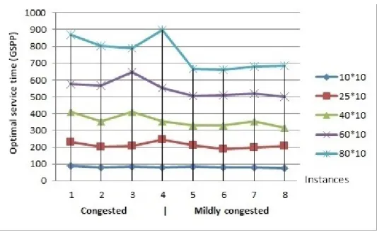
In Figure 4.1, the optimal service times have been plotted for each instance size with varying levels of congestion determined by the inter-arrival times of vessels. Two cases are considered; congested and mildly congested. From the figure, it is clear that as the instance size grows the effect of congestion is also higher as indicated by the negative slopes of the curves for the larger instances. Thereby it can be deduced that the temporal proximity of vessel arrivals enhances the complexity of the problem, and leads to higher service time values.
Figure 4.1: Effect of congestion on service times
For the column generation algorithm, we note that #iter indicates the number of it-erations of the column generation process to converge to the solution of the RMP, while # columns indicates the final number of columns generated. As discussed earlier, the solution value obtained from the column generation method provides a lower bound to the original problem and it is indicated by lb. The upper bound is obtained by running the RMP with integer decision variables at the end of the column generation method and it is indicated by ub. In the tables of results shown, gap represents the optimality gap between the lower bound and the upper bound while time represents the computation time in minutes and seconds. It can be seen from table 4.4 that for instances A, B and C with |N| = 10, 25 and 40 respectively, the gap values are equal to 0.00 % which indicates that the optimal solution is obtained directly from the column generation method for all congested and mildly congested instances except instance C1 where the gap is 0.16%.
45 Computation times are less than 1 minute for these instances excluding congested in-stances C1, C2, C3 and C4 where computation times are more than 1 minute but less than 3 minutes. For large instances with |N| = 60, 80, 100 and 120, the results show that the algorithm is able to solve all mildly congested instances to optimality in computa-tion time of a few minutes. Note that for congested instances, the optimality gap is very small and the highest computation time is only a little over 15 minutes for the congested instance G4.
From the results shown in Tables 4.4 and 4.5, it is interesting to note that the optimal-ity gap is zero or very close to zero for all instances. This means that for each instance, the pool of active columns at the end of the CG process contains the set of feasible columns that correspond to the optimal (or near optimal) solution. for |N| = 10, 25 and 40 vessels, the optimal solution is obtained directly from the column generation. For the other instances, given that the optimality gap is close to zero, we have not implemented branch and bound to further close the gap.
Table 4.6 shows that computation results obtained from the column generation al-gorithm with the improvement technique for congested instances E, F and G did not look very promising. It is clear that there has not been any significant improvement in computation time for these instances.
In light of the above results, the performance of the column generation algorithm proposed in this work to solve large size instances of the BAP is remarkable. Moreover, we note that the master problem is modeled as GSPP, the approach offers several
model-ing advantages, primarily because it is much easier to incorporate more advanced spatial and temporal constraints on individual vessels as these can be easily handled while gen-erating feasible assignments. It is also easier to model complex objectives as long as they can be expressed as a function of the column costs. Thus, the proposed column generation framework can be adapted to solve any variant of the BAP based on other spatial and temporal attributes.
47 Instance Congestion MIP SP CG |N |=10, |M |=10 obj g ap time(s) obj time(s)(H= 120) # iter # columns lb ub g ap time(H= 120) A1 Y es 88 0.00% 0.403 88 1.105 9 34 88 88 0.00% 7s A2 Y es 81 0.00% 0.276 81 0.692 4 20 81 81 0.00% 3s A3 Y es 84 0.00% 0.235 84 0.854 8 21 84 84 0.00% 6s A4 Y es 79 0.00% 0.508 79 0.806 7 40 79 79 0.00% 7s A5 Mild 84 0.00% 0.298 84 0.716 5 26 84 84 0.00% 4s A6 Mild 79 0.00% 0.198 79 0.730 2 11 79 79 0.00% 1s A7 Mild 80 0.00% 0.234 80 0.755 6 21 80 80 0.00% 4s A8 Mild 75 0.00% 0.340 75 0.741 5 18 75 75 0.00% 3s |N |=25, |M |=10 obj g ap time(s) obj time(s)(H= 120) # iter # columns lb ub g ap time(H= 120) B1 Y es 233 0.00% 8.008 233 2.027 9 121 233 233 0.00% 23s B2 Y es 204 0.00% 2.110 204 2.139 7 116 204 204 0.00% 18s B3 Y es 207 0.00% 6.785 207 2.229 10 134 207 207 0.00% 28s B4 Y es 244 0.00% 1708.224 244 2.078 13 183 244 244 0.00% 39s B5 Mild 213 0.00% 0.630 213 1.989 6 49 213 213 0.00% 9s B6 Mild 186 0.00% 0.803 186 2.073 5 53 186 186 0.00% 7s B7 Mild 200 0.00% 1.266 200 2.009 8 81 200 200 0.00% 15s B8 Mild 208 0.00% 1.776 208 1.921 8 65 208 208 0.00% 12s |N |=40, |M |=10 obj g ap time a(s) obj time(s)(H= 168) # iter # columns lb ub g ap time(H= 168) C1 Y es 420 13.67% -411 7.418 16 393 410.33 411 0.16% 2m11s C2 Y es 355 2.33% -355 6.639 11 277 355 355 0.00% 1m23s C3 Y es 415 6.12% -411 4.719 14 365 409 409 0.00% 1m37m C4 Y es 356 3.60% -355 6.711 13 275 355 355 0.00% 1m38s C5 Mild 332 0.00% 6.108 332 4.702 6 122 332 332 0.00% 22s C6 Mild 330 0.00% 13.698 330 4.961 10 126 330 330 0.00% 37s C7 Mild 356 0.00% 8.536 356 4.217 11 150 356 356 0.00% 40s C8 Mild 315 0.00% 3.252 315 6.158 9 102 315 315 0.00% 32s |N |=60, |M |=10 obj g ap time a (s) obj time(s)(H= 168) # iter # columns lb ub g ap time(H= 168) D1 Y es 602 14.27% -574 11.747 15 518 572.25 577 0.83% 2m57s D2 Y es 589 14.25% -565 9.54 16 560 564.6 565 0.07% 3m7s D3 Y es 709 25.01% -648 10.547 20 630 645.8 649 0.50% 3m53s D4 Y es 561 8.49% -554 10.107 16 428 554 554 0.00% 2m49s D5 Mild 505 0.01% 56.381 505 9.056 8 200 505 505 0.00% 44s D6 Mild 515 3.80% -508 7.942 13 247 508 508 0.00% 1m7s D7 Mild 518 0.01% 424.157 518 8.517 10 242 518 518 0.00% 1m3s D8 Mild 498 0.00% 34.767 498 9.204 8 186 498 498 0.00% 45s T able 4.4: Computational comparison between the algorithms for instances A, B, C and D a"-" indicates that the CPLEX time limit of 1800 seconds w as reached. b "+" indicates that the CPLEX solv er ran out of memory .
Instance Congestion MIP SP Dynamic CG |N |=80, |M |=10 obj g ap time a (s) obj time(s)(H= 168) # iter # columns lb ub g ap time(H= E1 Y es 956 27.04% -867 27.251 20 1012 858.85 870 1.30% 5m41s E2 Y es 900 24.17% -801 13.511 22 830 793.75 798 0.54% 5m31s E3 Y es 836 16.46% -791 24.143 18 807 788.75 791 0.29% 4m28s E4 Y es 830 15.63% -797 24.036 15 690 794.5 796 0.19% 3m29s E5 Mild 666 0.01% 620.353 666 9.454 12 292 665.5 666 0.08% 1m9s E6 Mild 663 0.01% 760.616 663 10.192 13 373 663 663 0.00 % 1m22s E7 Mild 679 0.01% 77.305 679 9.418 15 229 679 679 0.00 % 1m25s E8 Mild 686 0.01% 206.189 686 8.603 10 229 686 686 0.00 % 53s |N |=100, |M |=10 obj g ap time a (s) obj b time b (s)(H= 240) # iter # columns lb ub g ap time(H= F1 Y es 1208 28.22% -+ + 27 1066 1023.97 1031 0.69% 12m33s F2 Y es 1160 26.01% -+ + 22 954 1012 1016 0.40 % 9m17s F3 Y es 1377 35.70% -+ + 17 1169 1014 1016 0.20 % 7m33s F4 Y es 1025 20.20% -+ + 19 951 926.9 927 0.01% 7m57s F5 Mild 850 0.96% -+ + 9 366 849 849 0.00% 2m1s F6 Mild 857 2.64% -+ + 9 362 852 852 0.00% 1m55s F7 Mild 919 6.04% -+ + 14 428 897 897 0.00 % 2m53s F8 Mild 793 0.34% -+ + 9 304 793 793 0.00% 1m38s |N |=120, |M |=10 obj g ap time a (s) obj b time b (s)(H= 264) # iter # columns lb ub g ap time(H= G1 Y es 2565 59.43% -+ + 25 3339 1315.172 1321 0.44% 9m32s G2 Y es 1667 39.15% -+ + 22 1410 1201.533 1206 0.37% 13m20s G3 Y es 1569 32.33% -+ + 17 1234 1255.5 1257 0.12% 11m9s G4 Y es 1681 42.34% -+ + 23 1383 1137.75 1146 0.73% 15m9s G5 Mild 1016 1.04% -+ + 12 407 1014 1014 0.00 % 3m18s G6 Mild 994 1.51% -+ + 11 384 988 988 0.00 % 2m44s G7 Mild 1053 3.59% -+ + 10 409 1040 1040 0.00 % 2m36s G8 Mild 935 0.37% -+ + 10 306 935 935 0.00 % 2m34s T able 4.5: Computational comparison between the algorithms for instances E, F and G a "-" indicates that the CPLEX time limit of 1800 seconds w as reached. b "+" indicates that the CPLEX solv er rans out of memory .
49 Inst. CG (one column retrie v ed per subpr oblem) CG (5 columns retrie v ed per subpr oblem) CG (10 columns retrie v ed per subpr oblem) #iter #columns lb ub g ap time #iter #columns lb ub g ap time #iter #columns lb ub g ap time E1 20 1012 858.85 870 1.30% 5m41s 25 1809 858.99 868 1.05% 7m11s 23 1998 858.606 867 0.98% 6m 38s E2 22 830 793.75 798 0.54% 5m31s 18 1239 793.5 794 0.06% 4m37s 21 1404 794.25 797 0.35% 5m 33s E3 18 807 788.75 791 0.29% 4m28s 20 1288 788.5 791 0.32% 5m00s 19 1407 789 791 0.25% 9m 5s E4 15 690 794.5 796 0.19% 3m29s 17 1146 795.5 797 0.19% 6m9s 15 1133 794.75 797 0.28% 3m 34s #iter #columns lb ub g ap time #iter #columns lb ub g ap time #iter #columns lb ub g ap time F1 27 1066 1023.97 1031 0.69% 12m33s 19 1653 1023.7 1030 0.62% 12m33s 22 1926 1023.166 1030 0.67% 10m 14s F2 22 954 1012 1016 0.40% 9m17s 18 1590 1013 1017 0.39% 9m17s 19 1658 1012.15 1016 0.38% 8m 30s F3 17 1169 1014 1016 0.20% 7m33s 17 1899 1013 1013 0.00% 7m33s 19 2142 1013.04 1016 0.29% 8m 41s F4 19 951 926.9 927 0.01% 7m57s 16 1222 926.75 927 0.03% 7m57s 16 1240 926.75 927 0.03% 6m 49s #iter #columns lb ub g ap time #iter #columns lb ub g ap time # iter # columns lb ub g ap time G1 25 3339 1315.172 1321 0.44% 9m32s 25 3339 1315.172 1321 0.44% 9m32s 32 3961 1332.995 1362 2.18% 21m 48s G2 22 1410 1201.533 1206 0.37% 13m20s 22 1410 1201.533 1206 0.37% 13m20s 22 2689 1199.166 1204 0.4% 13m 17s G3 17 1234 1255.5 1257 0.12% 11m9s 17 1234 1255.5 1257 0.12% 11m9s 20 2428 1255.5 1257 0.12% 12m 46s G4 23 1383 1137.75 1146 0.73% 15m9s 23 1383 1137.75 1146 0.73% 15m9s 23 1383 1137.75 1146 0.73% 15m 9s T able 4.6: Results obtained from the CG with the impro v ement technique for congested instances E, F and G