HAL Id: inserm-00184247
https://www.hal.inserm.fr/inserm-00184247
Submitted on 30 Oct 2007
HAL is a multi-disciplinary open access archive for the deposit and dissemination of sci-entific research documents, whether they are pub-lished or not. The documents may come from teaching and research institutions in France or abroad, or from public or private research centers.
L’archive ouverte pluridisciplinaire HAL, est destinée au dépôt et à la diffusion de documents scientifiques de niveau recherche, publiés ou non, émanant des établissements d’enseignement et de recherche français ou étrangers, des laboratoires publics ou privés.
Computational modeling for systems biology and
physiology through examples
Alfredo Hernandez, Antoine Defontaine, Virginie Le Rolle, S. Randall
Thomas, Jean-Louis Coatrieux
To cite this version:
Alfredo Hernandez, Antoine Defontaine, Virginie Le Rolle, S. Randall Thomas, Jean-Louis Coatrieux. Computational modeling for systems biology and physiology through examples. Y. Gonzalez and M. Cerrolaza. Bioengineering Modeling and Computer Simulation, CIMNE, pp.121-159, 2007. �inserm-00184247�
COMPUTATIONAL MODELING FOR SYSTEMS
BIOLOGY AND PHYSIOLOGY THROUGH EXAMPLES
Alfredo I. Hern´andez1, Antoine Defontaine1, Virginie LeRolle1, S. Randall Thomas2 and Jean-Louis Coatrieux1
1 INSERM U642. LTSI Universit´e de Rennes 1 Campus de Beaulieu. 35042 Rennes, France 2IBISC FRE 2873 CNRS. Universit´e d’Evry Val d’Essonne 91000 Evry - France
Abstract. Although recent enthousiasm has emerged for Systems Biology, it is of major importance to identify the roots it has with computational (mathematical) modeling. In fact, major contributions have been made for decades with the aim to quantitatively analyze and model the function of living systems in order, ultimately, to better understand the underlying constituents and collective behaviors and use them for diagnosis and therapeutic purposes. However, the impressive evolution of technological resources and methods allows today to revisit these early attempts and to bring to light new concepts, targets, and expectations. This chapter, after a tentative definition of the generic elements behind Systems Biology and Physiology, will provide a review of current efforts devoted to multimodal, multilevel, multires-olution approaches, all being addressed from the joint observational, modeling and information processing points of view. The several theoretical frames at our disposal will also be addressed, in particular the capability to handle multiple modeling for-malisms. Examples from the literature and the research conducted by the authors will exemplify these multidisciplinary developments and results. The forthcoming challenges to be faced will then be outlined.
Key words: Systems biology, Physiology, Multiscale modeling, multiformalism, simulation.
HAL author manuscript inserm-00184247, version 1
HAL author manuscript
1 INTRODUCTION
Historically, the observation, analysis and understanding of biological and phys-iological processes have been based on experiments performed in vivo or in vitro. These experiments have mainly been carried out on animals, at a variety of ob-servation scales (subcellular, cellular, tissue, organ or system levels) giving rise to an exponentially growing number of data sets (genomics, proteomics, biomedical signal and image databases, etc.). These large data sets remain specific to a given scale of observation or experimental framework, and classical statistical tools usu-ally used for the analysis of these data are increasingly showing their limitations. The joint analysis of these data, taking into account the strong integration of bio-logical processes from the gene to the whole organism, represents one of the major research challenges for the coming years. New analysis frameworks and disciplines are currently emerging in order to cope for the complexity of this challenge.
Systems Biology is focused on the analysis of intra- and intercellular dynamics, mainly directed, at this point, by a semi-quantitative, statistically-based bottom-up approach, willing to cover from genotype to phenotype. The final objective in systems biology is to integrate the information on biological data sets and analysis methods into a generic, systemic and predictive approach1. Some of the most visible developments, such as the E-cell2 and Virtual Cell3 projects, are biophysical and biochemical in nature, and related to subcellular scales where proteins, substrates and product solutes, and ions interact to provide quantitative or semi-quantitative descriptions of cell level functions. Almost none of these projects currently provide kinetic descriptions linking cellular events to gene signaling and to regulation of transcription and translation, although the structuring of the protein-protein rela-tionships is proceeding rapidly by diagramming associations.
The Physiome Projects4,5, are based on a quantitative biophysical and determin-istic approach to describe molecular, cellular, organ and overall system behavior in an attempt to establish a top-down or a ”middle-out”6path to meet up with the ge-nomic and proteomic information and so provide a path that can be understood the whole way from Gene to Health. Focused efforts on particular Physiome projects, such as the ”Cardiome” project or those on kidney7,8 and lung modeling, represent current attempts in this direction. A recent special issue of the Proceedings of the IEEE has been entirely focused on the current developments of this project9.
These two complementary viewpoints for the comprehension of living systems, coexist by means of socially related but scientifically independent projects on in-tegrative systems physiology and biology. They share a number of methodological frameworks for the observation of living systems (constitution of data workbenches), creation of appropriate ontologies and for modeling and processing the observed data, and make them available to a large research community. Although these methodological frameworks have evolved in an impressive manner during the last years, many theoretical and technological issues remain to be addressed in order to achieve a coherent, fully functional approach.
This chapter will firstly point out the main difficulties associated with the quanti-tative study of biological and physiological systems. A brief description of a pioneer-ing effort to overcome these difficulties will be presented, followed by a presentation of a general framework (integrative modeling), currently in development to help
handle the complexity of living systems. Section 3 will present a contribution to a particular problem for the development of integrated models, related to the cou-pling of models defined in different mathematical formalisms. Some applications of this method, mainly on the analysis of the cardiovascular system function, will be presented in section 4. Finally, a discussion will outline the forthcoming challenges to be faced.
2 COMPLEXITY OF BIOLOGICAL AND PHYSIOLOGICAL SYS-TEMS
Biological and physiological systems appear particularly complex when compared to man-made ”artificial” systems encountered in traditional engineering fields (au-tomatics, electronics, industrial processes, etc.). This complexity is associated with a combination of different aspects: i) the limited knowledge of the underlying mech-anisms governing biological and physiological systems; ii) the diversity of spatial and temporal scales involved; iii) the variety of physico-chemical phenomena and energy domains, iv) the high level of interdependence between different biological functions, and v) the presence of non-linear processes and non-stationary situations. For instance, the cardiac activity is initiated by a biochemical process at a sub-cellular scale that generates the electrical activation of cardiac cells. Modifications of the intra and extracellular concentrations of calcium during this electrical activation, trigger the mechanical contraction of cardiac fibers and, then, the contraction of the whole ventricle. This pump action allows the circulation of blood in the vascular system, which irrigates the whole of body. All these active processes require energy to function and thus rely on a proper transport and management of metabolic agents. Moreover, all this activity is regulated by the Autonomic Nervous System (ANS) in a constant manner.
In the following sections, the most important aspects related to the complexity of biological and physiological systems will be breifly described and an emerging framework designed to tackle this complexity will be presented.
2.1 Diversity of spatiotemporal scales
Processes involved in the function of biological systems span a wide range of spa-tial and temporal scales. The spaspa-tial scales range from the gene (∼ 10−10m) to the whole body (∼ 1 m), that is to say one variation of about 1015. Temporal scales also show a variation of about 1015, going from the dynamics of ion channels in the cell (∼ 10−6s) to a whole life (∼ 109s). In general, the smallest scales are characterized by more important inter-individual variations than the larger scales. For example, the human body is constituted of10: more than 35000 different genes; more than 100000 kinds of proteins; more than 300 kinds of cells; 4 kinds of tissues: connective (cartilage, bones, blood, . . . ), epithelial, muscular, and nervous tissues; 12 differ-ent systems: cardiovascular, digestive, endocrine, excretory, immune, integumdiffer-entary (skin, hair and nails), lymphatic, muscular, nervous, reproductive, respiratory, and skeletal systems; 1 body.
2.2 High level of interdependence
Living systems are characterized by the presence of vast networks of interactions that, by synergy, let emerge new mechanisms which are much more complex than the simple, independent function of the different elements which constitute them. For example, functional networks emerge from gene and protein networks and their in-teractions with the intra- and extracellular spaces. The consequences of a particular gene modification on the physiology of a cell, or a whole organ, depend on the way in which this gene is involved on the various layers of integrative networks, from the sub-cellular scale to the highest scales. Many questions concerning Systems Biology are related to information processing, transduction pathways, the types of reactions, the non-linear relations involved, the effects of multiple regulatory loops, etc. This high level of interdependencies is also evident when trying to provide insight into the plausible roles of network topologies (chains, lattices, fully-connected graphs), on the mutual synchronization of cells (uniform or non-uniform pulse-coupled oscil-lators), traveling waves and non-linear dynamics, etc. All these issues are of concern for the Physiome and justify an effort to bring them to convergence.
2.3 Diversity of physico-chemical phenomena and energy domains Another source of complexity is related to the variety of energy domains in-volved in physiological processes. Indeed, a variety of physico-chemical phenomena are at the origin of the main physiological functions, such as regulation, growth, metabolism, electric and mechanical activities, etc. A quantitative analysis of these functions requires an appropriate formalization of the different energy domains (bio-chemical, hydraulic, mechanical or electric), and the coupling between these energy domains (such as the mechano-hydraulic function of the ventricles) must be correctly represented.
2.4 How to deal with this complexity?
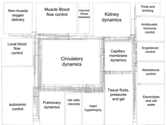
An approach that has proven to be particularly useful since the early attempts to harness the complexity of living systems is based on mathematical modeling. An interesting example of this model-based approach is the pioneering work of Guyton, Coleman and Granger11 for the analysis of the overall regulation of the cardiovascu-lar system. This model is composed of 18 ”blocks” representing the most relevant physiological sub-systems involved in cardiovascular regulation (Figure 1). Each of these blocks is composed of different sub-blocks (354 for the whole model) that rep-resent one or more mathematical operators or equations defining a particular aspect of the cardiovascular regulatory function, by using mainly a continuous transfer-function formalism. More than 150 variables related to cardiovascular transfer-function are simulated and their values are used as input/output data between the different model blocks.
Although this model represents only a basic description of the cardiovascular regulatory system, its simulation results have been used to reproduce and analyze the effect of specific circulatory stresses and pathologies or even to predict behaviors that were only observed experimentally later on. The success of this model was mainly due to the fact that it allowed a simultaneous analysis of the main components of the complete regulatory system and that it facilitated the representation and
Figure 1: Simplified diagram of the original Guyton 1972 model of the overall regulation of the cardiovascular system. Each block represents a major physiological organ or function. Lines between the blocks represent the input/output relations in the model
integration of new physiological knowledge. It was also used to identify in which parts of the system new knowledge is required, helping to propose new experimental investigations.
However, the authors already highlighted in their paper two major limitations of their approach: i) the impossibility of including different levels of anatomical detail within the same model and ii) the difficulties of handling the variety of temporal scales of the different components of the system. For example, long-term regulatory effects of cardiovascular activity (such as the renin-angiotensin-aldosterone system) present time constants measured in hours or days, while the short-term regulation (mainly by the baroreflex) present time constants on the order of the second. These aspects have been partly solved during the past decades with the evolution of com-puting power and research on modeling methodologies.
In particular, current research in ”integrative modeling” seeks to cope with the complexity of biological systems by means of a multiscale mathematical modeling approach12. This approach takes into account, in the same model, different physio-logical phenomena occurring on various scales, by using a common representation, defined comprehensively at the most detailed level. Multiscale models of cardiac function have been proposed in the literature by considering the interactions be-tween the sub-cellular level, the electrical activity and the mechanical activity of cardiac cells13,14. These models of global cardiac function have proven useful in a number of applications. However, their all-inclusive nature makes them difficult to
use in a concrete clinical application, because they require significant data-processing resources. For example, a cardiac model representing both ventricles with a reso-lution of 260,000 nodes and using a relatively simple model of the cardiac action potential, characterized by 12 parameters, requires more than 12 Gb of RAM for just the parameters and state variables. Moreover, none of the existing multiscale models allows a complete consideration of the whole cardiovascular system (includ-ing its regulation), so choices and compromise have to be made, depend(includ-ing on the intended application.
2.5 Integrative Modeling
McCulloch and Huber15proposed a graph representing the application of integra-tive modeling in physiology, based on three different axes (Figure 2): i) structural integration, ii) functional integration and iii) data integration. The structural in-tegration spans from the gene to the whole body, covering different spatio-temporal scales. The integration of different sources and physiological systems (i.e. electrical activity, mechanical activity, regulation,...) is represented in the ”functional inte-gration” axis. Finally, the data integration axis concerns the level of physical or physiological knowledge included in the model. One end of this axis corresponds to observational models (black-box models), which are limited to the reproduction of observations, and the other end corresponds to models integrating the most detailed physical and physiological knowledge available.
We have completed this representation by projecting into this space a number of different formalisms used in the literature for modeling the cardiovascular system. An analysis of this graph shows that there is a relationship between the formalisms used and the position of the models in this space. For example, the regulation of cardiovascular activity by the ANS is considered on the ”systems” level and is often modeled, based on experimental data, by a set of continuous transfer functions (TF). The electrical activity of the heart can be modeled at different levels of detail, going from the cell to the whole organ, and is usually represented by means of continuous, dynamical systems models (i.e. based on Ordinary Differential Equations) or by discrete models, (i.e. a set of coupled automata). However, both views still suffer from difficulties that reduce their clinical applicability: the former approach requires heavy computational resources while the latter does not permit the reproduction of certain pathologies defined at different scales.
Coupling models based on different formalisms (multi-formalism modeling) ap-pears as a way to overcome the practical limitations of existing multiscale mod-els16,17. In this context, one can easily think that a way to take advantage of the benefits of each approach in a model-based system would be to selectively define different regions of the modeled organ at different scale levels, depending on its physiological or pathological state. Such a multiresolution consideration is also le-gitimated by the practical clinical diagnosis performed by the physician, which aims at refining progressively the investigated region, going from a global consideration of healthy parts to a precise analysis of pathological sources. In the following sec-tion, the problem of multiformalism modeling is posed and an original methodology allowing the combination of different types of description formalisms will be pre-sented17,18.
Population Gene Regulation of cardiac activity Growth Metabolism Electrical activity Mechanical activity TF BG CA SDE MM PN ODE PDE AR Experimental data Physical principles
Figure 2: 3D space costituted by the three principal axes of integrative modeling proposed by Mc-Culloch et al. The vertical axis corresponds to structural integration, the diagonal axis represents data/knowledge integration and the horizontal axis represents functional integration. We have projected on this space various formalisms used in the modeling of the electrical and mechanical activities of the heart and the regulation of the cardiovascular activity by the autonomic nervous system. The formalisms shown in the figure are: AR – Autoregressive models, TF – Transfer function, BG – Bond Graph, CA – Cellular Automata, SDE – Stochastic Differential equation, MM – Markov Models, PN – Petri nets, ODE – Ordinary Differential Equations and PDE – Partial differential equations
3 TOWARDS AN INTEGRATED MULTIFORMALISM MODELING APPROACH
Several generic modeling and simulation tools are currently available. Matlab / Octave / Simulink, Berkeley Madonna, COMSOL and Mathematica are among the most commonly used. In such generic environments, a model is often composed of a set of coupled elements and a unique simulator is responsible for the simulation of this coupled model. Traditional simulators are usually based on a centralized approach where all the processing is done at the same level and, usually, inside a unique simulation loop which can solve only one modeling formalism. As a result, the integration of elements presenting different formalisms remains tricky (even when possible). Moreover, such tools often present an additional computing overhead due to their internal representation of each element of the model (e.g. use of an interpreted language) making them ineffective for the simulation of complex systems. Multiformalism modeling is an active research field, focused on the proposal of new architectures for an optimized representation and simulation of hybrid models (e.g. models constituted of coupled sub-models, defined with different mathematical formalisms). Two different approaches for multiformalism modeling can be distin-guished19–21:
• Formalism transformation: This approach seeks to transform all the sub-models presenting different formalisms into a common ”meta-formalism”, for which a simulator exists. Perfect analytical transformations exist between some continuous formalism, such the transformation of Bond-Graphs or con-tinuous transfer functions to an ODE system; however, these conversions are not always invertible and may demand an important effort.
• Co-simulation: The general idea behind co-simulation approaches is to pro-cess each sub-model with a specific simulator, adapted to the formalism in which it has been developed. The output of the general system is performed by a ”container” model, which assures an appropriate coupling between the different state variables. The main difficulty of this approach is precisely to define the appropriate spatial and temporal coupling relations.
A third approach, combining formalism transformation and co-simulation, has also been proposed21, but it can clearly be considered as a particular co-simulation system. An interesting co-simulation approach for multiformalism modeling has been proposed by Zeigler22. It is based on a distributed architecture with two main characteristics:
• a tree-like hierarchy with different modeling layers: each leaf is an ”atomic” model (e.g. a single sub-model) and ”coupled models” represent a gathering of different kinds of models (atomic or already coupled models);
• a parallel between a model hierarchy and the correspondng simulators: each atomic model is associated with a simulator adapted to its formalism. For example, a continuous simulator will be associated with an atomic continuous model and a discrete simulator would be associated with a discrete atomic model.
Various research projects have emerged that aim to make practical implementa-tions of the initial theoretical aspects presented by Zeigler. These projects are often based on the use of a common discrete-event system specification (DEVS) formal-ism for the simulation of hybrid systems and, in particular, for the simulation of continuous systems using discrete-event simulators. In order to perform the spa-tial and temporal couplings between sub-models defined with different formalisms, piecewise linear or polynomial approximations of continuous values23 or a quantiza-tion of the values obtained from the different sub-models24–26 have been proposed. A modification of the original Zeigler’s architecture has also been proposed with the introduction of a unique level in the hierarchy27. QSS and VLE are the most active projects on the field26,28.
Nevertheless, all of these projects impose the application of a unique DEVS sim-ulator and often lack a modular object-oriented representation of each sub-model. We were thus motivated to develop an original object-oriented approach allowing the use of standard simulators from the literature for each formalism. This is par-ticularly important when integrating biophysical models from different authors, as these models are often accompanied by specific simulators. Zeigler’s original archi-tecture, as proposed in22, and the co-simulation method have been retained for our development. This approach presents several advantages: i) it is particularly suited for the creation of generic multiformalism modeling tools, ii) it facilitates the dis-tributed execution of the coupled simulators in a computer cluster and iii) it eases the extension of the method to a multiresolution model representation.
As mentioned above, the main difficulty associated with a multiformalism mod-eling approach based on co-simulation concerns the coupling mechanisms between components defined with different formalisms. The following section will state the problem of the definition of an appropriate coupling method and the methodological choices retained for the development of our system.
3.1 Spatial coupling and temporal synchronization
The combined simulation of atomic models defined by different formalisms im-poses the definition of specific methods for spatial coupling and temporal synchro-nization. This problem may be stated as follows: Let model M be defined as:
M(F, I, S, P ) (1) where F is the description formalism, I is a set of one or more inputs, S are the state variables and P are the internal model parameters. It is obvious that the choice of an appropriate simulator for model M depends on the components of the model (I, S and P ) and, thus, on formalism F . Indeed, the nature of the representations of the model components depend on F and may be, for example, boolean, quantized, discrete or continuous.
The co-simulation approach that we have retained is based on a parallel between a model M and its corresponding simulator. A specific simulator for formalism F can be represented as:
O = SimF(M(F, I, S, P ), Ps) (2) where M is the model associated with simulator SimF (and described by the same formalism F ), Psare the simulation parameters and O are the outputs of the model,
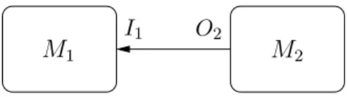
M1 M2 O2
I1
Figure 3: M2’s output as M1’s input
obtained by simulation. A coupled co-simulation of two models M1 and M2, defined respectively by formalisms F1 and F2, in which the outputs of M2 are used as inputs to M1 can thus be represented as follows (figure 3):
O1 = SimF1(M1(F1, T(O2), S1, P1), Ps,1) (3)
O2 = SimF2(M2(F2, I2, S2, P2), Ps,2) (4)
One of the most important aspects of co-simulation is thus to define a trans-formation T permitting to solve relation 3. A definition of such a transtrans-formation considering temporal and spatial aspects is presented in the following sections. 3.1.1 Spatial coupling
Experience shows that the definition of spatial coupling of two models represented by different formalisms is problem-specific. In particular, it depends on the nature of the different elements (discrete or continuous) and the way they are linked to-gether. For instance, in the previous example 3, two models M1 and M2 are coupled with M2’s output (O2) corresponding to M1’s input (I1). If O2 is discrete while I1 expects continuous values, a simple sample-and-hold method can be used between two consecutive simulation steps. Linear or higher-order interpolations can also be considered. If O2 is continuous while I1 expects discrete values, quantization meth-ods could be used. A concrete example of this point will be presented in the next section, illustrating the characteristics of the proposed approach.
3.1.2 Temporal synchronisation
The simulation of mono-formalism models implies the evaluation and update of state variables at a set of predefined time instants. Most of the currently available generic commercial simulators define the interval between these time-instants (sim-ulation steps) as fixed or adaptive, but they are the same for the whole sim(sim-ulation process.
In the case of the co-simulation of a coupled multi-formalism model, each atomic model is processed by a particular simulator, that may have an independent simu-lation step. The evolution of each atomic model M can be obtained, for example, by using the traditional Euler method:
SM(t) = SM(t − 1) + δtM · ∂Sm
∂t (t) (5) where δtM represents the temporal simulation step-size for atomic model M. De-pending on the numerical method used, this step can either be fixed or adaptive.
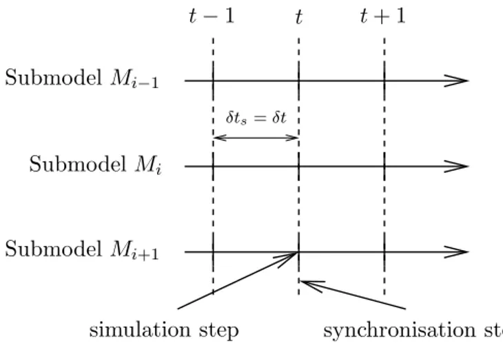
Even if each atomic model evolves with its own simulation step (i.e. with proper time characteristics and dynamics), a temporal synchronization δts is necessary be-tween the different coupled models, in order to obtain the global simulation outputs. Three types of temporal synchronization can be distinguished to deal with the dif-ferent dynamics of the difdif-ferent elements. They are depicted in figures 4 - 6, where we consider three coupled atomic models, Mi−1, Mi and Mi+1. These three synchro-nization methods are:
• Simulation with a fixed time step and synchronisation at each time step (figure 4): In this approach, the simulation step is δt for all the elements, independently of their local dynamics. This is the simplest way (which is indeed the same used in mono-formalism simulators) but it takes no advantage of using models with slow or fast dynamics.
• Synchronization at a fixed time step and simulation with adaptive step (figure 5): Here, each atomic model evolves with its own simulation step (one or more iterations) between two consecutive synchronization time steps. The objective is to exploit the different dynamics of the atomic models. For in-stance, a model showing slow dynamics (Mi) presents higher simulation steps (δti) than a model (Mi+1) with faster dynamics (δti+1). Using this approach implies to define which value should be used to update coupled elements be-tween two consecutive synchronization steps. A sample-and-hold method has been retained. In this method, the coupling between atomic models is updated through a fixed synchronization step. The definition of this fixed synchroniza-tion step is done in a similar manner as in tradisynchroniza-tional fixed-step methods. • Update and synchronization at the smallest time step required by
any of the atomic models (figure 6): As in other rate-adaptive methods, this approach requires the calculation of the optimal simulation step for each atomic model, before performing the update of state variables. In this case, the smallest step size is used for all the atomic components and for the syn-chronization. For instance, at time t, each element (Mi−1, Mi or Mi+1) requires an optimal step such as δti+1 < δti−1 < δti. Simulation, and therefore syn-chronization, of the elements will consequently be performed according to the time step δt = δti+1.
It should be noted that the last two methods, with variable simulation steps, are only possible using a distributed co-simulation architecture. In a centralized method, the first synchronization method is the only one possible. Finally, the combination of the two adaptive methods can be considered, especially for systems whose elements show dynamics with important disparities.
4 SOME EXAMPLES ON CARDIAC PHYSIOLOGY
The proposed approach for multiformalism modeling and simulation has been evaluated and applied in a number of different biomedical applications29–31. The evaluation is based on i) the construction of equivalent monoformalism and multifor-malism models, ii) the simulation of these models with the proposed multiformultifor-malism library using different simulation parameters and iii) a comparison of the simulation
Submodel Mi−1
Submodel Mi
Submodel Mi+1
t −1 t t+ 1
δts= δt
simulation step synchronisation step
Figure 4: Fixed-step simulation and synchronisation
Submodel Mi−1 Submodel Mi Submodel Mi+1 t −1 t t+ 1 δts δti+1
simulation step synchronisation step
Figure 5: Synchronisation at fixed step (δts) and adaptive simulation of each submodel
Submodel Mi−1 Submodel Mi Submodel Mi+1 t −1 t t+ 1 δti−1 δti δts= δti+1
estimated simulation step for cell i
synchronisation step
Figure 6: Adaptive synchronisation and simulation
results from the two approaches and an analysis of the simulation properties, such as computation time.
In this section, an example of the validation of the proposed multiformalism approach is presented, by comparing mono and multiformalism models of normal and pathological cardiac tissues, defined at the cellular level. A second example shows the integration of discrete and a variety of continuous formalisms in a multi-resolution model of the circulatory system.
4.1 Monoformalism models of cardiac tissues
The classical implementation of monoformalism models of cardiac tissues can be realized in two steps. In a first step, continuous atomic models of the electrical activity of single cardiac cells are created. The second step concerns the definition a cardiac tissue, with a given 2D or 3D geometry, composed of a set of coupled atomic models, as defined in the previous step.
A number of electrophysiological models of cardiac cells, based on a Hodgkin Huxley framework32, has been proposed in the literature33–36. Most of these models represent different cell types (e.g. from the sinoatrial node, atria, Purkinje fibers, ventricles) of animal hearts (e.g. rabbit, canine, guinea pig), mainly because these experimental models are the most accessible. Recent improvements have led to models of human cells34,37 and to a finer representation of the dynamics of the dif-ferent ion channels, linking the molecular and cellular levels36. In the literature, ”black-box” morphological cardiac models based on a FitzHugh Nagumo frame-work38 have also been proposed39 but they present only a limited interest when dealing with physiopathological parameters. In current large-scale models such as the CARDIOME project, thousands of cells are coupled in a predefined geometry to represent one or more cavities of the heart, thus covering the molecular to organ levels36. Due to this extensive definition, these models require massive computing resources that limit their direct clinical application.
For this example, we have chosen the Beeler and Reuter (BR) model, that rep-resents cardiac ventricular cells in the physiological case40. A model of an ischemic myocyte, adapted from the Beeler Reuter model by Sahakian41has also been imple-mented to take into account membrane current modifications of this pathology. The coupled tissue-level model is thus composed of a set of coupled atomic submodels (BR or Sahakian models) in a 2D or 3D geometry.
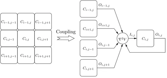
In order to apply the proposed co-simulation approach, a continuous simulator is associated with each atomic BR model. A ”simulation coordinator” is responsible for the coupling between all atomic models and the global simulation of the whole system. Coupling between cells has been defined in order to produce an isotropic propagation, as depicted if figure 7. In the coupled model, the behavior of state variable Vi,j, representing the membrane potential of cell Ci,j is given by:
dVi,j
dt = G(Pi,j) + K · ∇ 2V
i,j (6)
where G(Pi,j) is a set of equations describing the cellular behaviour (e.g the complete set of Beeler and Reuter model equations40) and K is a diffusion coefficient between neighbouring cells42. Due to spatial discretisation, the Laplacian ∇2V
i,j is estimated
Ci,j Ci,j Ci−1,j−1 Ci−1,j Ci−1,j Ci−1,j+1 Ci,j−1 Ci,j−1 Ci,j+1 Ci,j+1 Ci+1,j−1 Ci+1,j Ci+1,j Ci+1,j+1 Coupling Oi,j Oi−1,j Oi+1,j Oi,j−1 Oi,j+1 Ii,j ∇2V
Figure 7: Schematic implementation of the coupling method: the Laplacian (∇2V) is
calcu-lated at the coupled model level while the obtained value is added to the external inputs (I) of the correspondind submodel (Ci,j)
t1= 4 ms t2 = 8 ms t3 = 12 ms t4 = 16 ms
−85 mV 50mV
Figure 8: Depolarisation front for healthy tissue: left column of cells are stimulated by a plane stimulus
by:
∇2Vi,j = 1
h2(Vi+1,j+ Vi−1,j+ Vi,j+1+ Vi,j−1−4Vi,j) (7) where h corresponds to the spatial quantification scale introduced by the application of finite differences.
In our co-simulation architecture, the Laplacian is calculated at the tissue level and the obtained value is introduced as an external input current (I in (1)) for the corresponding atomic model Ci,j (figure 7). Border conditions of the tissue consist in a null flux and diffusion coefficient K has been set such that the propagation velocity is physiologically coherent.
4.1.1 Healthy tissue
Using tissue definition as previously described, square simulated tissues of 256 x 256 cardiac cells defined by Beeler and Reuter model (representing approximately 10 x 10 mm) have been implemented. Propagation of the action potential is shown in figure 8; it corresponds to a planar depolarization front propagating from left to right.
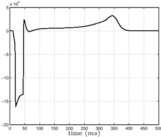
0 50 100 150 200 250 300 350 400 450 500 −20 −15 −10 −5 0 5x 10 4 time (ms)
Figure 9: Dipolar projection for a healthy tissue over the propagation axe
Figure 9 represents the equivalent dipolar projection over the propagation axe. Although it cannot be considered as an electrocardiogram (ECG) or an electrogram (EGM), some ECG’s markers are present: QRS complex during depolarisation or T wave during repolarization.
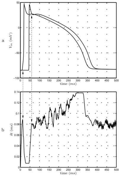
The three synchronisation methods proposed in the previous section have been evaluated. Using fixed step synchronisation and adaptive simulation of atomic sub-models (figure 5) instead of fixed step simulation and synchronisation (figure 4) shows a calculation time decreased by a factor of 8.8. Using adaptive synchronisa-tion (figure 6) shows gains of a factor of 27.3. It is to note that this last method allows to take into account different dynamics occurring during the action potential propagation. Figure 10 represents action potentials for the first and the last column of the tissue with the corresponding synchronisation steps. Steps are small dur-ing depolarisation, which presents fast dynamics, whereas they are more important during repolarisation where variations are slower.
4.1.2 Ischemic tissues
The previous definition of healthy tissues can easily be adapted to define other types of tissues and, in particular, ischemic tissues. In this example, some atomic models representing the Beeler and Reuter model on the middle of the tissue have replaced by the model proposed by Sahakian41 that reproduces the dynamics of ischemic cells. The model structure, the simulator and the coupling methods are generic and remain applicable.
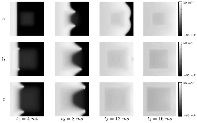
Different degrees of ischemia (20%, 40%, 60%) have been introduced for the cen-tral cells. A gradient of potassium concentration ([K+]) from normal to pathologic levels has been defined so as to produce a gradual difference of resting potential and avoid spontaneous depolarizations. Figure 11 represents depolarization fronts for different instants. Analysis of these fronts corresponds to observations made in is-chemic pathology43: i) quicker depolarization at the border zone; ii) depolarization block at the center of the ischemic zone; iii) modification of the depolarization front in the shadow of the ischemia and iv) quicker repolarization of ischemic cells.
0 50 100 150 200 250 300 350 400 450 500 0 0.02 0.04 0.06 0.08 0.1 0.12 0.14 0 50 100 150 200 250 300 350 400 450 500 −100 −50 0 50 time (ms) time (ms) δ t (m s) Vm (m V ) a b
Figure 10: a) Action potentials for the first and last column of cells in a healthy 2D tissue. b) Evolution of the adaptive simulation/synchronisation step δt for the global simulator. Note that the smallest δt values are used only during the depolarization of the whole tissue (indicated with the arrows). Once the first row of cells starts repolarizing, showing slower dynamics, the value of δt is progresively increased
t1= 4 ms t2 = 8 ms t3 = 12 ms t4 = 16 ms a b c −85 mV −85 mV −85 mV 50mV 50mV 50mV
Figure 11: Depolarisation fronts for tissues presenting a) 20%, b) 40% and c) 60% of ischemic cells
Using the same approach as such presented for 2D tissues, 3D tissues can be de-fined in a straightforward manner, such as in figure 12, which represents the propa-gation of the depolarization front in a cube of 64 x 64 x 64 cells (2.5 x 2.5 x 2.5 mm), with a central ischemic region. This approach can be directly used to define a given anatomical geometry representing both ventricles, or the whole heart. However, al-though the proposed co-simulation approach presents lower simulation times than classic, centralized approaches, this exhaustive representation at the cellular level, based on continuous models still requires significant computational resources. This point is clearly a limitation of the continuous monoformalism approach. The next subsection concerns precisely the definition of equivalent multiformalism models that help to reduce these computational resources.
4.2 Multiformalism models of cardiac tissues
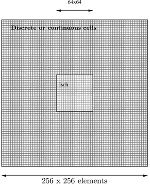
In this section, hybrid tissues, composed of both continuous and discrete atomic submodels, have been defined. Peripheral cells in the tissue are represented by cellular automata and central cells by continuous models, such as depicted in fig-ure 13. The coupled model structfig-ure is similar to those previously presented for the monoformalism case.
A convenient discrete atomic model of the electrical activity of cardiac cells has been developed in our laboratory44. This model is composed of four physiological states corresponding to the different phases of an action potential (figure 14): i) idle, ii) rapid depolarization, iii) absolute refractory period and iv) relative refractory period. These automata possess two main dynamical properties: refractory period dependence to the stimulation frequency as well as the response to premature
t1 t2 t3
Figure 12: Extension of the proposed approach to the 3D case. Example of the propagation of depolarization front for a 3D tissue presenting an ischemic central region. An acceleration in the borders of the ischemic region is visible at instant t = 2ms, alteration of the propagation front behind the ischemic area is observable at instant t = 4ms and repolarisation of ischemic cells has begun at t = 6ms
000000000000000000000 000000000000000000000 000000000000000000000 000000000000000000000 000000000000000000000 000000000000000000000 000000000000000000000 000000000000000000000 000000000000000000000 000000000000000000000 000000000000000000000 000000000000000000000 000000000000000000000 000000000000000000000 000000000000000000000 000000000000000000000 000000000000000000000 000000000000000000000 000000000000000000000 000000000000000000000 000000000000000000000 111111111111111111111 111111111111111111111 111111111111111111111 111111111111111111111 111111111111111111111 111111111111111111111 111111111111111111111 111111111111111111111 111111111111111111111 111111111111111111111 111111111111111111111 111111111111111111111 111111111111111111111 111111111111111111111 111111111111111111111 111111111111111111111 111111111111111111111 111111111111111111111 111111111111111111111 111111111111111111111 111111111111111111111 000000 000000 000000 000000 000000 000000 111111 111111 111111 111111 111111 111111 64x64 Isch
Discrete or continuous cells
256 x 256 elements 10 x 10 mm
Figure 13: General scheme of multiformalism tissues
UDP ARP RRP Idle extStim TU DP(t) +∆U DP(t) TARP(t) +∆ARP(t) TSDD(t) > extSim TRRP(t)
Figure 14: Different states of each myocardial cellular automata. Each state corresponds to a tissue-level physiological state: idle (resting potential), UDP rapid depolarization, ARP absolute refractory period and RRP relative refractory period
tivations44. In order to cope with spatial coupling problems, this model presents a continuous output (O in (1)) defined by a piecewise linear interpolation of a Beeler and Reuter action potential (figure 15).
In such hybrid tissues, as previously introduced, the main issue lies in the defini-tion of a spatial coupling method that guaranties acdefini-tion potential propagadefini-tion and especially at the interface between models of different formalims. As a reminder, coupling is performed by a Laplacian seen as an external current, as previously implemented for continuous models, while it is done by transmission of a flag for discrete models18. Spatial coupling of such hybrid models concerns precisely the definition of a link between those two approaches.
In order to cope with this problem, we propose a new multiformalism coupling method for cardiac electrical activity, based on the definition of a novel coupling function CoupF.. Let C
F.
i,j be an atomic cell component of a cardiac tissue, defined by formalism F.(where F.can be continuous Fc or discrete Fd). The generic coupling behaviour (membrane potential, Vi,j) can be extended from (6) as follows:
Vi,j is given by GF.(Pi,j) + CoupF.(K · ▽
2V) (8)
where GF. is a function of parameters P (either for the discrete or continuos model),
CoupF. is the coupling method defined and K is the diffusion coefficient as defined
in (6). The coupling method can be defined as follows: CoupF. =
(
thres if the cell model is discrete(F.= Fd)
id if the cell model is continuous(F. = Fc) (9) where id is the identity function (coupling method as previously introduced for con-tinuous models) and thres is a threshold function setting external activation for the
0 50 100 150 200 250 300 350 400 450 500 −100 −80 −60 −40 −20 0 20 40 time (ms) m em b ra n e p ot en ti al (m V )
Figure 15: Continuous output of cellular automata obtained by a piecewise linear fitting of a Beeler and Reuter model
cellular automata if the input is greater than the limit value obtained previously (3.5 mA). Depolarisation of a Beeler and Reuter model has been studied for differ-ent values of input currdiffer-ent, and it has been shown that there is a minimum value (3.5 mA) above which depolarisation occurs. This threshold has been retained for activation of discrete models.
4.2.1 Healthy tissues
Action potential propagation on healthy tissues has been studied for three types of models:
• the continuous monoformalism model (BR) defined by Beeler and Reuter cells presented in the previous section (used as reference);
• a monoformalism discrete tissue model (CA) defined by cellular automata; • a hybrid model (CABR) where peripheral cells are discrete and the 64 x 64
central cells defined by Beeler and Reuter model.
Depolarization fronts for these three different models are presented in figure 16. The differences between the simulations obtained from these three models are pre-sented as point to point absolute error between the reference (BR) tissue and the other tissues (figure 17). This error is mainly due to the morphological differences between the outputs of discrete and continuous atomic models and the fact that discrete information is used to propagate the wavefront through cellular automata. However, in all cases the global physiological behavior at the tissue level (conduction velocity, propagation properties, etc) is preserved.
Using a hybrid approach instead of a monoformalism one reduces up to 4 times the computation times. In total, a gain factor of 90 is observed using a hybrid model with adaptive synchronisation when compared to a continuous tissue with fixed stepped simulation and synchronisation.
t1= 4 ms t2 = 8 ms t3 = 12 ms t4 = 16 ms a b c −85 mV −85 mV −85 mV 50mV 50mV 50mV
Figure 16: Depolarisation fronts for healthy tissues: a) monoformalism continuous BR tissue, b) monoformalism discrete CA tissue and c) hybrid CABR tissue. The global physiological behavior at the tissue level (conduction velocity, propagation properties, etc) is equivalent for the three models
t1= 4 ms t2 = 8 ms t3 = 12 ms t4 = 16 ms a b 0mV 0mV 45mV 45mV
Figure 17: Point to point absolute error for healthy tissues: a) between BR and CA and b) between BR and CABR. These differences are mainly due to the different morphologies of the action potentials of discrete and continuous models (see figure 15)
replacemen t1= 4 ms t2 = 8 ms t3 = 12 ms t4 = 16 ms a b −85 mV −85 mV 50mV 50mV
Figure 18: Depolarisation fronts for ischemic tissues: a) BRIsch tissue, b) CAIsch tissue
t1= 4 ms t2 = 8 ms t3 = 12 ms t4 = 16 ms
0mV 45mV
Figure 19: Differences between depolarisation fronts for ischemic tissues
4.2.2 Ischemic tissues
Ischemic tissues have also been simulated in both continuous (BRIsch) and hybrid (CAIsch) cases (figure 18). The typical behaviour of ischemic tissues is simulated in both cases, with abnormal and incomplete depolarisation in the ischemic zone, quicker depolarisation at the border, depolarisation block at the center, modification of the depolarisation front in the shadow of the ischemia and quicker repolarisation. Point-to-point differences are also presented in order to quantify the alteration of the simulation using the hybrid approach instead of the continuous one (figure 19). Although differences appear in the shadow of the ischemia, due to differences in morphologies as well as quantification of the coupling term for discrete submodels, these results show a sufficiently approached response for a global clinical description. 4.3 Multiformalism and multiresolution model of the cardiovascular
sys-tem
The analysis of the autonomic nervous system (ANS) activity and, particularly, of the way it modulates the cardiovascular system has been shown to provide effective markers for risk-stratification and early detection of cardiac pathologies45,46. In clinical practice, the analysis of the ANS is commonly performed by applying a set
of tests called autonomic maneuvers. However, the interpretation of these tests can be very difficult, due to the multidimensionality of the observed phenomena, and the fact that the complex mechanisms involved in the autonomic regulation of the cardiovascular system are not fully understood. Physiological models can be of a particular interest in this context.
In this section, we present a model-based approach for the analysis of the short-term autonomic regulation of the cardiovascular system. The proposed model takes into account the following subsystems: i) the cardiac electrical activity ii) the car-diac mechanical activity (and the electro-mechanic coupling), iii) the circulatory system and of course iv) the autonomic baroreflex loop, including afferent and ef-ferent pathways. Although difef-ferent models have been proposed in the literature for each of these components, treated independently, only a few models combining all three components have been proposed. One of the difficulties for the development of such a model is related to the fact that different energetic domains are involved in the cardiovascular system function and its regulation. As shown in figure 2, dif-ferent formalisms can be used to create the model in order to take into account this variety of energy domains and consider the different sub-systems that constitute the CVS. In this work, we combine the following formalisms into a global model of the short-term regulation of the cardiovascular system:
• the Bond Graph formalism, because it facilitates both the integration of dif-ferent energy domains (e.g. hydraulic and mechanic) and the construction of a global system of the CVS47;
• continuous ODEs, for the representation of the electrical activity at the cellular level;
• continuous transfer functions are employed for the representation of the dif-ferent modules of the autonomic baroreflex;
• discrete cellular automata, to reproduce the cardiac electrical activity at the tissue-level.
The proposed multiformalim modeling approach has thus been particularly use-ful for the definition of the model. Moreover, in order to better represent some pathophysiological mechanisms, different resolutions of the vascular system and the ventricular models have been proposed in a multi-resolution model. The following sections will present each of the model components, their integration in a global model, and simulations for the analysis of Valsava maneuvers and Tilt tests.
4.3.1 Model of the ventricles
The cardiac contraction is at the origin of the transport of blood in the circula-tory system. At the scale of cardiac cells, the contraction is due to the shortening and lengthening of sarcomeres, which are the elementary mechanical contractile ele-ments. This mechanical activity is under the influence of an electrical activity, since the variation of the calcium concentration during the action potential allows the development of force in the sarcomere.
Different models of the ventricular contraction have been presented in the litera-ture. The most detailed models are often based on a network of connected (finite) elements that allow a relatively precise description of the structure and function of the myocardium. As already stated, these models are difficult to use in clinical practice, mainly due to the computing resources required. Simpler models of the ventricular contraction have also been presented, representing each ventricle as a sin-gle adaptive elastance48–50. The main advantage of this approach, which is related to their low computational costs, is the fact that they can be easily integrated into a model of the complete CVS. This kind of model has also been shown to provide a satisfying behaviour in response to physiological variations51 (change of position, temperature, physical activity. . . ). However, although these models provide good global descriptions of the contraction, the influence of calcium concentration during the contraction process and the regulation by the ANS are not taken into account and, since the ventricle is represented with a single element, intra-ventricular desyn-chronizations cannot be represented.
In order to overcome these limitations, we have chosen to include a description of the electro-mechanical process, keeping the simplified representation of the ven-tricles provided by the elastance model. As a first approximation, the Beeler and Reuter model40, already presented in this chapter, has been used, as it presents a basic description of the intracellular calcium dynamics while keeping a low level of complexity. However, the BR model cannot be directly implemented under the Bond Graph formalism, due to its non-linearity and the strong interdependence between the state variables. This model has thus been implemented as a set of ordinary differential equations and coupled with the Bond-Graph model of the circulation by means of the proposed multiformalism approach.
The intracardiac calcium concentration variable of the BR model is used as input to a model of development of mechanical force in the cardiac muscle fibers. The model proposed by Hunter et al52 has been chosen because it gives a geometrical description of the cardiac contraction of the fibers. The stress in the fiber axis is obtained by adding these passive and active tensions:
Tf iber(l) = Tactive(l) + Tpassive(l) (10) The active tension is defined as being dependant on the fibre strain (l ) and the calcium concentration [Ca2+], in the following manner:
Tactive(l) = Tref(1 + β0(l − 1)).
([Ca2+])h ([Ca2+])h+ Ch
50
(11) where Tref is the reference tension at l = 1, [Ca2+] represents intracellular cal-cium concentration dynamics, obtained from an electrophysiological model of car-diac cells40, C50 is the intracellular calcium concentration at 50% of the isometric tension, h is the Hill coefficient and β represents the myofilament ”cooperativity” term. In the Bond Graph representation, this tension has been modeled by two ca-pacitive elements: one for the passive properties of the muscle and one for the active properties. The dynamics of each capacitive element are described by equations 10 and 11. A 1-element is used to join the two capacitive elements because the total tension in the axis of the fiber is the sum of two tensions (see figure 20).
Figure 20: Bond Graph model of the ventricle and its coupling with the BR action potential model
The rise of the force and the variation of the fiber length lead to variations of ventricular pressure and, thus, to the ventricular contraction. In this approach, the ventricle is assumed to be made of concentric rings of muscular fibers. So the ventricular pressure depends only on the tangential tension, which corresponds to the fibers axes. An empirical relation between fiber force and ventricular pressure has been proposed by Diaz-Zuccarini53, in which the ejected volume V is defined as a function of the fiber strain l by:
V = Aln (12)
where the values of A and n are empirically defined. This approach has been shown to provide simulation results that are coherent with physiology53. Neglecting energy losses of the ventricular contraction, the same empiric law holds to describe the relation between the fiber force and the ventricular pressure. As a result, the change of energy domain from mechanics to hydraulics can be described by a transformer implementing equation 12. A Bond-Graph representation of the model is shown in figure 20.
4.3.2 Model of the circulatory system
The circulatory system is composed of the systemic and the pulmonary circu-lations that respectively transport blood to bring the nutrients and oxygen to the organs, and permits the oxygenation of blood in the lung. These vascular systems are composed of different kinds of vessels called arteries, capillaries and veins. As proposed by other authors54, a segment of a vessel is modeled in this work as an RCL circuit, representing the resistive, capacitive, and inertial properties of a given vessel segment. Each segment is directly represented using the Bond-Graph formalism.
Figure 21: Bond Graph model of the circulation: a) a simple model distinguishing the pulmonary and systemic circulation b) a more detailed model differentiating the systemic circulation on the head, the abdomen and the legs
A number of segments of this kind are connected in series in order to model the whole circulatory system in a global, lumped-parameter representation. In order to analyze data from different autonomic tests, two configurations, showing different resolutions of the vascular system, have been proposed: a simple configuration dis-tinguishing only the pulmonary and systemic circulation (figure 21.a) and a more detailed representation in which the model of the systemic vascular tree has been divided in three parts (the head, the abdomen and the legs) (figure 21.b). The for-mer configuration is adapted to the analysis of autonomic tests in supine position (such as the Valsalva manoeuvre), while the latter can be used to study orthostatic responses (such as the tilt test). The heart valves are modeled as non-ideal diodes using modulated resistances. The atria are modeled as constant capacitances (fig-ures 21a and 21b). The ventricular model described in the previous section is used for the left and right ventricles.
The parameter values used in the model come from the literature55,56. For exam-ple, the values of the parameters of the aorta are: C=0.2199 ml/mmHg, R=0.0675 mmHg.s/ml and I=0.000825 mmHg.s/ml.
4.4 Model of the ANS
The autonomic nervous system (ANS) is the component of the nervous system that acts as the main modulator and control mechanism of internal organs, adjusting their activity to the requirements of the body as a whole and preserving homeostasis (rising the heart rate during exercise, for example). The short-term regulation of the CVS is mainly performed by the baroreceptor loop that plays an important role in blood pressure control, adjusting mainly the heart rate, heart contractility, and vessels constriction in order to maintain the systemic arterial pressure level within the physiological range. This adjustment is done by the two components of the ANS: the sympathetic and the parasympathetic systems.
Figure 22: a) components of the ANS model b) structure of each ANS regulation component
Models of the ANS are typically based on a continuous transfer function for-malism describing the different sub-systems that can be associated to an entity of the cardiovascular control57,58. Many of such models59,60 are based on a common structure, composed of delays and first order filters, allowing the description of the different response times of the sympathetic and the parasympathetic systems. The Van roon model59 has been retained in this work and coupled with the ventricular and the circulatory models proposed in the previous sections. This model takes into account the baroreflex, the cardiopulmonary reflex, with a separated representation for the baroreceptors, the pulmonary receptors, the Nucleus Tractus Solitarii (NTS) and the sympathetic and parasympathetic systems.
Four variables are controlled by this ANS model, by means of specific efferent pathways: heart rate, cardiac contractility, systemic resistance and venous volume (figure 22.a). The heart rate depends on the action of both the sympathetic and the parasympathetic systems. The contractility of the heart, the systemic resistance, and the venous volume are only under the influence of the sympathetic system. Each efferent pathway is based on the same model structure, composed of a delay and a first order filter, representing the particular neurotransmitter dynamics of that pathway (figure 22.b). The ANS model is coupled to the CVS by injecting in the latter the four previous controlled variables in the following way:
• Regulation of heart rate: The output signal of the heart rate regulation model is continuous. To obtain pulsating blood pressure, an IPFM (Integral Pulse Frequency Modulation) model is used, because it transforms a continu-ous input signal into an event series61. The input of the IPFM model is the output signal of the heart rate regulation model. The output of the IPFM al-lows the excitation of the BR model of electrical activity. Each emitted pulse results in an increase of calcium concentration.
• Regulation of cardiac contractility: The Tref parameter (equation 11) of the active tension of cardiac fiber can be considered to be an indicator of cardiac contractility. In this sense, we have replaced the Tref definition in equation (11) by the output signal of the contractility regulation model. • Regulation of systemic resistance: The value of the parameters of the
systemic resistance is replaced by the output signal of the resistance regulation model.
• Regulation of venous volume: The constitutive relation of the venous capacity depends on the unstretched volume Vo. The value of Vo in the venous
capacity is replaced by the output signal of the venous volume regulation model.
4.5 Simulation of the cardiovascular response to autonomic maneuvers Two of the most common autonomic maneuvers are the Valsalva maneuver62 and the Tilt test63. These maneuvers are based on the controlled modification of one cardiovascular variable, in order to observe the regulatory response of the ANS. Different observations, such as the electrocardiogram (ECG), the noninvasive systemic arterial pressure (SAP) or the respiration, are acquired concurrently, to better characterize this autonomic response. In this section, the proposed model of the CVS and its regulation by the autonomic nervous system is used to obtain simulations of the main observed variables during these two kinds of autonomic maneuvers. The simulations will be compared to actual physiological data acquired in our laboratory.
4.5.1 The Valsalva Maneuver
The Valsalva Maneuver is a non-invasive, non-pharmacological autonomic test, which is based on a forced expiration, to increase the intrathoracic pressure. In this protocol, the subject is placed in supine rest and asked to breath out through a bugle connected to a pressure measurement system. The subject is asked to main-tain a pressure of around 30 to 40 mmHg for a period of 15 seconds, after which a complete expiration is made. The Valsalva maneuver consists of 4 phases. The forced expiration causes an initial increase in blood pressure, and a slight increase in heart rate, due to the augmented intrathoracic pressure (phase I). During phase II, the augmented intrathoracic pressure reduces the volume of cardiac chambers (mostly the right heart), preventing cardiac filling and reducing the stroke volume and aortic pressure. This effect produces an unloading of the baroreceptors and an activation of the sympathetic nervous system, starting to increase heart rate and pe-ripheral vasoconstriction to balance the decreased aortic pressure. After expiration (phase III), a further sudden drop of aortic pressure is produced by the reduction in intrathoracic pressure. However, due to the effect of autonomic activation in phase II and the progressive restoration of hemodynamic conditions, the aortic pressure starts to rise. In phase IV, before reaching a normal physiological value, the blood pressure rises well above the original levels (overshoot phase), causing the loading of the baroreceptors and a vagal autonomic activation that leads to an abrupt drop in heart rate64.
For the simulation of a Valsalva maneuver, the simplest model of the circulation is used. The transmural pressure of thoracic vessels and of the cardiac cavity (ven-tricles, atria) is raised to simulate an augmentation of the intrathoracic pressure to a value of 40 mmHg. The model is simulated during 15 seconds, in order to obtain the heart rate and blood pressure signals. The obtained simulated signals are thus compared to real signals, acquired from normal subjects by using a ”Task Force Monitor” acquisition system (CNSystems, Graz, Austria).
Figures 23.a and 23.c show simulated signals and figures 23.b and 23.d present real data. In general, and from a qualitative standpoint, the model seems to reproduce the main cardiovascular behaviour during a Valsalva maneuver. It is possible to
Figure 23: Simulation of the response of the CVS to a Valsalva maneuver for blood pressure a) and heart rate c), real data of blood pressure b) and heart rate d)
recognize the four typical phases of the Valsalva maneuver on both the simulated and observed signals. Blood pressure dynamics reveal the rise during phase I, an increase and a decrease in phase II, a short fall in phase III and the return to normal conditions in phase IV. Note the consistent simulation of the overshoot period on phase IV. Heart rate dynamics are also consistent with the physiology, a slow increase of heart rate during Valsalva, which is followed by a decrease after expiration. However, it is possible to observe some differences between simulations and real data. They are mainly due to the fact that the parameters values used in these simulations are those presented in the literature, and were not adjusted for individual subjects.
4.5.2 Tilt Test
The head-up Tilt test focuses on the short-term regulation of the mean arterial blood pressure (MABP) by the ANS. It is usually employed for the detection of vasovagal syncope and consists of observing the variation of heart rate and blood pressure during the change of a patient’s position from a supine to a head-up posi-tion. During tilt, approximately 300 to 800 ml of blood may be shifted into the lower extremities, leading to a reduction of venous return and hence of stroke volume. In normal subjects, a decrease in the MABP causes the unloading of arterial
Figure 24: Comparison of simulated and observed data during a tilt test. Simulated blood pressure a) and heart rate c), real data of blood pressure b) and heart rate d)
ceptors, providing a sympathetic activation that leads to enhanced chronotropism (increased heart rate), inotropism (increased ventricular contractility) and periph-eral vasoconstriction. A balance is established between heart rate and contractility to maintain the cardiac output and MABP in physiological levels.
To simulate a tilt test, the second version of the model (differentiating the head, the abdomen and the legs) is used, in order to represent a pressure gradient on the systemic circulation. During a tilt test of a normal subject, an increase of the MABP of the order of ∆P = 25 mmHg and ∆P = 50mmHg are typically observed for the abdominal and leg circulations, respectively, while a decrease of ∆P = -30mmHg is measured at the level of the head. These values have been used to simulate a tilt test with the model, by introducing a modulated source of pressure in each compartment. Figures 24.a and 24.b show the simulated and the observed systolic blood pressures, as measured in the lower part of the body. It is possible to observe a sudden rise of blood pressure after the tilt, followed by a smooth decrease, due to autonomic regulation. Then, the pressure increases slowly. The influence of the autonomic regulation on heart rate is also studied. Figures 24.c and 24.d compare the simulated and the observed heart rate. It is possible to observe that the heart rate augments abruptly after the tilt, and slowly decreases when the blood pressure approaches its physiological values.
5 DISCUSSION AND PERSPECTIVES
Modeling can be seen as a major tool in order to integrate knowledge, to drive experiments, to optimize measurements in biological and clinical research. A key ob-jective behind modeling is also, by determining the deviations of model parameters in pathological states from their normal behaviors, to conjecture the reverse process, in other words, to derive ways to go back from abnormal to normal states and to assist in pathology diagnosis and the definition of optimal therapeutic actions. Coupling multiformalism and multiscale models are among the most challenging problems to address in order to apply this model-based approach to real-life situations.
An original generic approach for multiformalism modeling has been presented in this chapter, allowing the combination, in a single global model, of different types of models defined by different formalisms with proper spatial and temporal scales. This approach has been defined to cope with submodels characterized by wide ranging spatial and temporal dynamics and thus represents an initial step towards a feasible multiresolution framework for clinical applications. Examples of the application of this multiformalism approach have been shown, with models covering different scales:
• Models of the cardiac electrical activity presented in sections 4.1 and 4.2 inte-grate levels from cell to tissue. Different cardiac electrophysiological properties have been simulated in different types of tissues, showing the interest of the definition of hybrid, multiformalism models.
• The model of the cardiovascular system and its modulation by the autonomic nervous system presented in section 4.3 is an example of integration from tissue to system levels. It also shows the application of a multiresolution modeling, led by the clinical application of interest.
Validation results in both cases have highlighted that the qualitative clinical in-terpretations are preserved while using multiformalism models. Experiments have also shown a reduction of the computing time by a factor up to 87.3 while using mul-tiformalism models with the proposed temporal synchronisation methods instead of classical monoformalism simulation with fixed step integration. Though satisfactory, these results are still not sufficient for practical use in a clinical context.
As has been pointed throughout this chapter, most of the issues to deal with are very challenging and require an important international research effort. It is our feeling however that this is only a limited part of the whole landscape. Let us look forward to what should be explored in the near future. This we will do by revisiting a classical and fundamental epistemological loop (figure 25), familiar to experimen-talists (especially biologists and physicists). This iterated loop applies of course to many research domains dealing both with artificial (human-made) and natural systems but is, in our experience, much more complex for living systems. A unidirec-tional traversal of this loop may seem evident. We start with a hypothesis (intuition or idea), design the experimental platform and a specific protocol that hopefully allow testing it, define the sensing devices required, process the data and interpret the results. This straitghtforward path, where a number of internal connections are not represented, is much more difficult to define than we first imagined.