HAL Id: hal-02894662
https://hal.telecom-paris.fr/hal-02894662
Submitted on 9 Jul 2020
HAL is a multi-disciplinary open access
archive for the deposit and dissemination of
sci-entific research documents, whether they are
pub-lished or not. The documents may come from
teaching and research institutions in France or
abroad, or from public or private research centers.
L’archive ouverte pluridisciplinaire HAL, est
destinée au dépôt et à la diffusion de documents
scientifiques de niveau recherche, publiés ou non,
émanant des établissements d’enseignement et de
recherche français ou étrangers, des laboratoires
publics ou privés.
Efficient Scheduling of FPGAs for Cloud Data Center
Infrastructures
Matteo Bertolino, Andrea Enrici, Renaud Pacalet, Ludovic Apvrille
To cite this version:
Matteo Bertolino, Andrea Enrici, Renaud Pacalet, Ludovic Apvrille. Efficient Scheduling of FPGAs
for Cloud Data Center Infrastructures. Euromicro DSD 2020, Aug 2020, Portorož, Slovenia.
�hal-02894662�
Efficient Scheduling of FPGAs for Cloud Data
Center Infrastructures
Matteo Bertolino
⇤, Andrea Enrici
†, Renaud Pacalet
⇤, Ludovic Apvrille
⇤ ⇤LTCI, Télécom Paris, Institut Polytechnique de Paris, France†Nokia Bell Labs France, Centre de Villarceaux, 91620 Nozay, France
firstname.lastname@{telecom-paris.fr, nokia-bell-labs.com} Abstract—In modern cloud data centers, reconfigurable devices
can be directly connected to a data center’s network. This con-figuration enables FPGAs to be rented for acceleration of data-intensive workloads. In this context, novel scheduling solutions are needed to maximize the utilization (profitability) of FPGAs, e.g., reduce latency and resource fragmentation. Algorithms that schedule groups of tasks (clusters, packs), rather than individual tasks (list scheduling), well match the functioning of FPGAs. Here, groups of tasks that execute together are interposed by hardware reconfigurations. In this paper, we propose a heuristic based on a novel method for grouping tasks. These are gathered around a high-latency task that hides the latency of remaining tasks within the same group. We evaluated our solution on a benchmark of almost 30000 random workloads, synthesized from realistic designs (i.e., topology, resource occupancy). For this testbench, on average, our heuristic produces optimum makespan solutions in 71.3% of the cases. It produces solutions for moderately constrained systems (i.e., the deadline falls within 10% of the optimum makespan) in 88.1% of the cases.
Index Terms—Dependency graph scheduling, Resource
con-strained scheduling, Cloud data center, FPGA
I. I
In modern cloud data enters, FPGAs are directly connected to the data center’s network and are accessible as stand-alone resources [1]. Here, FPGAs are rented to users to accelerate the execution of data-intensive workloads, e.g., scientific com-puting, financial analysis, video processing, machine learning. This motivates the study of new scheduling algorithms that maximize the utilization, hence profitability, of FPGAs (i.e., minimize latency and reduce resource fragmentation). Scheduling on FPGA systems is a classical resource-constrained scheduling problem (RCSP). It consists of execut-ing a workload of = tasks ) with a start and end C0, C=+1
tasks, respectively. Each task is associated to a processing time F8 during which no interruption is allowed. The 8C ⌘task
may start only once its predecessors are finished (the network of preceding tasks is assumed to be acyclic - a dependency acyclic graph, DAG). Resources are needed to execute the workload: a set of resources is given, task C8 requires A8:
units of the :C ⌘ resource each time it executes. At each time
instant, ': units of resource : are available. The goal of this
classical RCSP problem is to determine a start and finish time for each task such that the workload’s makespan (the
The work in this paper is funded by Nokia Bell Labs France. It is part of an academic partnership between Nokia Bell Labs France and Telecom Paris on Models and Platforms for Network Configuration and Reprogrammability.
finish time of C=+1) is minimized. For a taxonomy of RCSPs
problem, we invite the reader to consult the work in [2]. The authors in [3] demonstrated that the classical RCSP problem is a strongly NP-hard problem. Thus, much attention has been dedicated by the FPGA community to the design of heuristics. In this paper, we propose an efficient heuristic for FPGA scheduling. The rationale behind our heuristic is to iteratively transform an input DAG, with multiple execution orders, into a totally ordered DAG. At each iteration, we form a group of tasks, that we call a slot, by contracting task nodes in the current DAG. Groups are formed by considering tasks’ resource needs around a high-latency task that executes in parallel to lower-latency tasks, thus hiding their latency. Slots are sequentially executed, interposed by FPGA total recon-figurations; tasks in slot < start execution when all tasks in preceding slots have completed. We compared our algorithm to the Next-Fit version of the well-known and performing heuristic Heterogeneous Earliest Finish Time (HEFT) [4]. We show that HEFT-NF is outperformed in terms of quality (i.e., the number of solutions that coincide with the optimum) without compromising runtime. In the rest of this paper, Section II discusses related work. Section III presents our system models and design assumptions. Section IV describes our heuristic. Section V discusses evaluation results, before the conclusions and future work in Section VI.
II. R
Scheduling heuristics that use a static model (i.e., a DAG whose characteristics are known beforehand) can be classified as list-based, pack-based and clustering. We exclude from our discussion meta-heuristics (e.g., Genetic Algorithms, Tabu Search) as we propose a heuristic which is also based on the processing of a DAG, similarly to existing heuristics. Our solution’s runtime is typical of heuristics, i.e., tens of mil-liseconds (see Section V), whereas meta-heuristics normally require seconds or minutes to produce a solution [5]. In list scheduling [6]–[8], individual tasks are sorted in a priority list and assigned, in sequence, to the earliest available unit that fits their resource request. Priorities can be assigned statically or dynamically based on different characteristics, e.g., execution time, resource occupancy. List heuristics are very popular, they require very small runtimes in exchange for the optimality of the output schedules.
computation of more expensive priorities but yield higher-quality schedules. Similarly to our work, in pack scheduling, tasks are packed together and packs are executed sequentially. Within a pack, tasks can execute in parallel; a pack cannot start before all tasks from previous packs have completed execution. Numerous contributions (see [9] and its related work) target High-Performance Computing platforms without reconfigurable hardware. To the best of our knowledge, only the work in [10] proposes a pack-based solution for FPGAs. Here, resources are abstracted as a single parameter, area. An FPGA area is partitioned in slots, tasks are divided in groups and each group is scheduled to one slot with the Earliest Deadline First policy. With respect to our work, the authors in [10] consider independent tasks and a 1D resource model. Pack heuristics are related to the bin-packing problem and its variants. Bin-packing is similar, in principle, to FPGA scheduling: items’ volumes correspond to tasks’ resources and bins correspond to FPGA execution steps/slots. However, the main goal of bin-packing is to minimize the number of bins, which does not necessarily translate into minimizing an application’s makespan: few high-latency bins may require more time to execute than a larger set of low-latency bins. Based on the same rationale as pack scheduling are clustering heuristics, that originate in compilers for parallel machines. Because of the limited space we only mention [11] that is one of the most cited heuristics. Here, groups of tasks called clusters are created, from the dependency graph of some input code, so as to minimize the overall code’s execution time. Specific to some solutions in this domain is task duplication: a task may have several copies in different clusters and each copy is scheduled independently. Duplication is not at all a desirable feature in our work: users who rent one or more FPGAs would have to pay also for the resources occupied by duplicate tasks. Another difference is the lower level of granularity that is typical of tasks in clustering algorithms: tasks can be routines or even subparts of routines. To the best of our knowledge, no heuristic exists that forms clusters around high-latency tasks, as we propose in this paper.
Server-based scheduling is a recent technique from the real-time community [12] that groups tasks in so-called servers. In [12], a server is defined as a periodic task whose purpose is to serve aperiodic requests for resources as soon as possible. Static server-based scheduling for FPGAs was first studied in [13] for independent periodic tasks. On-line server-based scheduling is described in [14], [15], in the context of a real-time operating system, also for independent tasks. Our work differs from [13]–[15] as (i) we account for task dependencies and (ii) we provide a generic model for : resources whose requests are constant in time and independent of task schedul-ing.
III. S
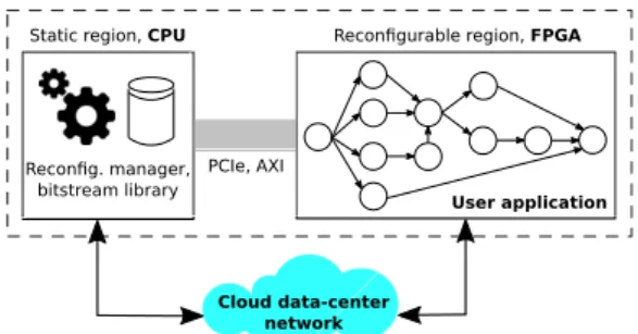
With respect to classical RCSPs, our problem is further complicated by task dependencies, hardware reconfiguration and the fact some resources depend on the task scheduling itself. In our work, we target platforms, Fig. 1, that
are composed of two logical parts: a static region and a reconfigurable region, interconnected by a bus-based infrastructure. The static region executes on a general-purpose processor, in charge of running the reconfiguration management and a reconfigurator device that internally reconfigures the system at runtime. The reconfigurable region is composed of a reconfigurable hardware device that is entirely assigned to a user by a network orchestrator (e.g., according to some service-level policy). This assignment is
Static region, CPU
Reconfig. manager, bitstream library
PCIe, AXI
Reconfigurable region, FPGA
Cloud data-center network
User application Server
Fig. 1. The architecture of a modern FPGA-based server.
fixed for the entire execution of a user’s workload. Modern FPGAs, such as those deployed in cloud data centers, offer multiple types of physical resources to allocate tasks. Resources are available in different quantities, packaged in different ways (e.g., granularity of blocks) and with slightly different denominations according to the FPGA manufacturer and/or FPGA family. The basic units of an FPGA are blocks of reconfigurable logic, sometimes referred to as slices or logic cells. These are composed of flip-flops (registers) and Look-Up Tables (LUTs). FPGAs also offer pre-built digital signal processing blocks (DSPs), e.g., multipliers, to save on the usage of logic units and accelerate workloads such as scientific computing and signal processing. Memory resources are available, to store temporary results or communicate between tasks, in the form of Random Access Memory (RAM), both on-chip (e.g., Static-RAM) and off-chip (e.g., Dynamic-RAM). On-chip memory is also available in the form of configurable flip-flops. In the context of our work, for each workload, a user disposes of one or more bitstreams that are designed off-line either by the user or are available as part of a library developed by third-parties, e.g., the cloud provider, the FPGA manufacturer. We target the case where a user’s workload cannot execute in its entirety on a given FPGA and the latter must be reconfigured at least once. These assumptions are coherent with the design capabilities currently offered by FPGA manufacturers and vendors’ tools. A user’s workload is denoted (Fig. 1) as a DAG ⌧ =< ), ⇢ >. Each task C8 2 ) is mapped to the reconfigurable
region, it is a technologically mapped netlist implement-ing the 8C ⌘ task. We characterize it by means of a tuple
(⌘8, A81, A82, ..., A8:), where ⌘8 is the hardware execution time
(HET) that is the time taken by C8 to execute. The
tuple (A81, A82, ..., A8:), e.g., A81 is the number of logic blocks,
A82 is the amount of on-chip RAM, A83 is the number of DSP
blocks. Note that, for instance, for easier partial bitstreams composition, the logic block resource could very easily be replaced by entire rows of logic blocks. The occupancy of resources in the tuple is associated to an operating frequency. Multiple tuples for different operating frequencies can be assigned to a workload. Our heuristic supports aperiodic as well as periodic applications. We only require a workload graph to include: one instance of a periodic application’s dependency graph for each period to schedule; the precedence relations between tasks that belong to different periods. In the context of our work, as users rent cloud resources, they are always aware of their workloads’ characteristics on a target family of FPGAs. In other words, tasks’ resource occupancy is known beforehand, typically thanks to data available during the synthesis and simulation of a workload’s bitstream, profiling or interpolation and curve-fitting from historic data. Also task DAGs can be readily retrieved with the same techniques or simple static analysis of application code (e.g., dependency analysis available in compilers and hardware synthesis tools). Remaining design assumptions are listed below:
• All tasks are released at the same time instant, each with
a deadline that is equal to the entire workload’s deadline (i.e., the time granted to a user to dispose of the FPGA).
• The time to read, write and transfer the input/output data
for a task C in different memory locations is included in the task’s hardware execution time.
• Tasks require a fixed amount of resources and have a fixed
execution time (no moldable nor malleable tasks).
• The time to transfer a reconfiguration bitstream is
in-cluded in the FPGA total reconfiguration time )'.
IV. T
The formulation of our heuristic is generic and valid for :-dimensional models of resources whose requests are constant in time and do not depend on the scheduling of tasks. We consider a set that contains : resources, available in ': units. Each task C8 consumes a fixed amount of each
resource, A8: that does not vary with time. Our heuristic
takes scheduling decisions for groups of tasks that we call a
slot. A slot B is defined by the tuple (⌧B, ⌘B, AB1, AB2, ..., AB:).
⌧B ✓ ⌧ is the slot’s graph of tasks and ⌘B is the slot’s
HET. The generic tuple (AB1, AB2, ..., AB:) denotes the slot’s
occupancy for each of the : resources (e.g., number of logic blocks, memory, DSP blocks). Resources occupied by a slot correspond to the sum of the resources occupied by its constituent tasks. Obviously, the amount of a slot’s resources cannot be larger than those available in the target FPGA: AB1 = ÕC82⌧BA81 '1, AB2 = ÕC82⌧BA82 '2, ..., AB: = Õ
C82⌧BA8: ':. Slots are executed sequentially, tasks within a slot cannot execute until all tasks in preceding slots have terminated. Slots are interposed by FPGA reconfigurations that add a latency denoted by )'.
In synthesis, our heuristic iteratively transforms a DAG that expresses multiple partial execution orders into a DAG that expresses a single total execution order (a schedule). This is performed, at each iteration, by creating a slot, thanks to the concept of computational dominance. A slot is built around the task that has the largest HET (dominating task) among unscheduled tasks. Dominated tasks are added to a slot, as long as there are enough FPGA resources, in a way that reduces the parallelism for further slots the least possible. The final schedule is of a succession of FPGA configurations, whose latency is determined by that of the dominating tasks that hide the latencies of the dominated tasks. Algorithm 1 shows the heuristic’s pseudo-code. Its core is constituted by a loop, lines 5-14, that iterates over a worklist where tasks are sorted in decreasing order of their HET. At each iteration, the algorithm selects from the worklist a dominating task C8 and computes the set ( of candidate slots,
function 1D8;3⇠0=3830C4(;>CB(). For the sake of simplicity, we provide here an intuitive description of its behavior (see sub-section IV-B for the details). A candidate slot is composed of a dominating task C8 and a resource-feasible set of
domi-nated tasks. Such a set is composed of all combinations of tasks that can execute in parallel to C8 and fit the remaining
FPGA resources (i.e., the total FPGA resources minus those occupied by C8). For instance, let’s consider the DAG in Fig. 2a.
Let’s suppose that t3 is the dominating task and that both t2
and t5 can be allocated in the FPGA together with t3. Then,
there are 3 resource-feasible sets, {C2}, {C5}, {C2, C5}, and a set
of 4 candidate slots: ( = { {C3, C2, C5}, {C3, C2}, {C3, C5}, {C3} }. 1 Function generateSlots( ⌧ = < ), ⇢ > ): 2 ⌧0:= ⌧;/* Copy G to G’, G’=<T’,E’> */ 3 F>A :;8BC )0\ {C0, C=+1};/* C0= CB>DA 24, C=+1= CB8=: */ 4 F>A :;8BC
B>AC =⇡42A40B8=6$A 34A$ 5 ⇢)(F>A:;8BC);
5 foreach C82 F>A:;8BC do
6 ( ;;/* set of candidate slots */
7 ( 1D8;3⇠0=3830C4(;>CB(C8, ⌧0, (, '1, '2, ..., ':); 8 foreach B 2 ( do 9 B2>A4B[ B ] 2><?DC4(2>A4(B, ⌧0); 10 end 11 ⌧B A4CA84E4!>F4BC(2>A4(;>C(B2>A4B[]); 12 ⌧0 2>=CA02C(D16A0?⌘(⌧B, ⌧0); 13 F>A :;8BC F>A:;8BC \ {⌧B}; 14 end 15 return G’;
Algorithm 1: The slot scheduling heuristic
Among all candidate slots in (, only one is selected to be created in the current DAG ⌧0, lines 8-10 in Algorithm 1.
This selection is based on the score returned by function 2>< ?DC4(2>A4(B, ⌧0) that we detail in Algorithm 2. A score is an estimate of the makespan in the graph ⌧0 ⌧B that
would result if we created slot B and removed its tasks ⌧Bfrom
⌧0. This estimate is computed by separately considering inter-task dependencies and HETs, from the reconfiguration time
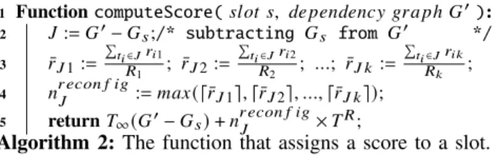
1 Function computeScore( B;>C B, 34?4=34=2H 6A0?⌘ ⌧0): 2 := ⌧0 ⌧B;/* subtracting ⌧B from ⌧0 */ 3 ¯A 1:= Õ C8 2 A81 '1 ; ¯A 2:= Õ C8 2 A82 '2 ; ...; ¯A : := Õ C8 2 A8: ': ;
4 =A 42>= 5 86:= <0G(d¯A 1e, d¯A 2e, ..., d¯A :e);
5 return )1(⌧0 ⌧B) + =A 42>= 5 86⇥ )';
Algorithm 2: The function that assigns a score to a slot. )' and the occupancy of tasks’ resources. This is motivated
by the fact that these elements are statistically independent. Hence, the two terms returned by Algorithm 2. The first term, )1(⌧0 ⌧B) quantifies the impact of tasks’ HET and inter-task
dependencies (that impose scheduling constraints), by ignoring resource occupancy. We compute it as the sum of the HETs for all tasks that lie on the critical path from source to sink, )1(), in the subgraph ⌧0 ⌧B. The second term is an estimate of the
number of reconfigurations, in the residual graph ⌧0 ⌧B. It is
computed by ignoring inter-task dependencies and considering the occupancy of the tasks’ FPGA resources only. It is denoted as =A 42>= 5 86 in Algorithm 2, where = ⌧0 ⌧
B.
Back to Algorithm 1, at line 11, we select the slot with the lowest score. This is the slot for which the estimated makespan in ⌧0 ⌧B is the lowest. Therefore, creating this slot leaves
the (estimated) highest degree of parallelism in the residual DAG ⌧0 ⌧B. Creating a slot is performed by contracting
the nodes for the slot’s tasks ⌧B into a single node, in ⌧0,
by function 2>=CA02C(D16A0?⌘(). The latter modifies ⌧0 by
relabeling nodes that belong to ⌧Bwith the new slot identifier.
It collapses the newly relabeled nodes by removing internal edges as well as duplicate cross edges (edges with an endpoint in the slot and one in ⌧0 ⌧B) and self-loops (edges whose
endpoints are identical). For instance, the contraction of tasks t2, t3, t5 in Fig. 2a results in the DAG on Fig. 2b.
We precise to the reader that, in Algorithm 2, function 2>< ?DC4(2>A4(B, ⌧0) does not modify ⌧0. Instead, function 2>=CA02C(D16A0 ?⌘(⌧B, ⌧0) returns a modified version of ⌧0
that, at line 12 in Algorithm 1, is used for the next iteration and overwrites the current ⌧0.
A. Example
We illustrate our heuristic on the example DAG in Fig. 2a. We target the FPGA Xilinx Spartan 7 XC7S25. We consider three types of resources: logic blocks A81 (called, for instance,
Configurable Logic Blocks - CLBs - in Xilinx’ nomenclature), DSPs A82 and on-chip RAM blocks A83 (BRAM in Xilinx’
nomenclature). In total, this FPGA disposes of 1825 CLBs, 80 DSPs and 45 blocks of BRAM (each block is 36 kbit large). The total reconfiguration time )' is 40 ms, for a
bitstream of 9934432 bits and a SPIx4 bus at 66 MHz. The resource occupancy of tasks C8 in Fig. 2a are given in Table I.
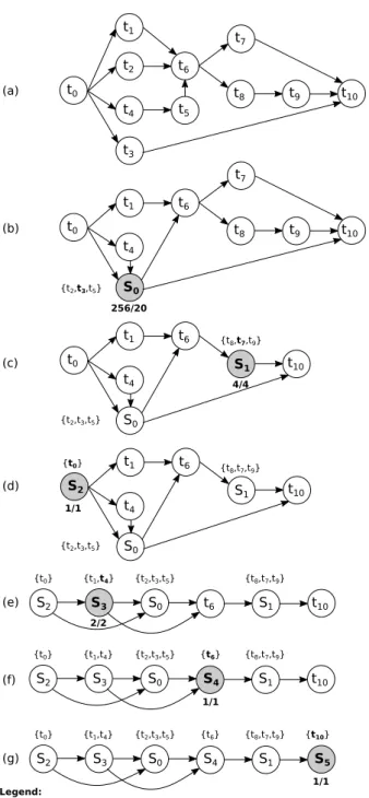
Fig. 2 illustrates all the graph transformations that the heuristic performs from a partially order DAG of tasks (Fig. 2a) to a totally order DAG of slots (Fig. 2g). Each transformation corresponds to an iteration of the for-loop in Algorithm 1. We highlight to the reader the usefulness of the score in Al-gorithm 2: it allows the heuristic to take scheduling decisions
that a user normally considers counter-intuitive. For instance, slot (0 = {C2, C3, C5} is preferred over 19 other resource-feasible
candidates, such as {C2, C3, C4}. When S0is created, it leaves the
highest degree of parallelism for the next graph transformation. While in {C2, C3, C4}, all tasks can execute in parallel, slot
{C2, C3, C5} amortizes the execution time of t5 (larger than that
of t4) as t5 can execute in parallel to t3 (dominating task).
In Fig. 2, all tasks within slots execute in parallel but for slot S1, where t7 executes in parallel to the sequence of t8, t9.
The total makespan of the slot DAG in Fig. 2g is 1763 ms: it is equal to the sum of the dominating tasks’ HET, plus the latency necessary to reconfigure the FPGA 5 times.
TABLE I
T HET F . 2
Task CLBs DSPs BRAM blocks HET [ms]
t0 344 23 4 287 t1 285 30 4 139 t2 192 18 9 209 t3 249 23 7 460 t4 429 6 11 200 t5 496 5 9 314 t6 665 17 6 199 t7 556 22 3 303 t8 400 5 3 35 t9 709 7 5 49 t10 206 10 12 114
B. The heuristic’s complexity
The complexity of the heuristic is determined by the creation of all candidate slots for a dominating task C8,
function 1D8;3⇠0=3830C4(;>CB() (line 7 in Algorithm 1) whose pseudo-code is presented in Algorithm 3. Candidate
1 Function buildCandidateSlots( C8, ⌧0= < )0, ⇢0> , (, '1, '2, ..., ':): 2 ⇠ ⌧0\ {C8, ?A43(C8, ⌧0), BD22(C8, ⌧0)}; 3 foreach ⇠02 2><18=0C8>=B$ 5 %0A0;;4;)0B:B(⇠) do 4 ⌧B= {C8}; 5 B ({C8}, ⌘8, A81, A82, ..., A8:); 6 5 40B81;4= CAD4; 7 foreach C22 ⇠0do 8 if 4G42DC8>=)8<4(⌧B+ C2, ⌧0) ⌘8 then 9 if 5 40B81;4 ;;>20C8>=(B, C2, '1, '2, ..., ':) then 10 B (⌧B+ C2, 4G42DC8>=)8<4(⌧B+ C2, ⌧0), AB1+A21, AB2+A22, ..., AB:+A2:); 11 2>=C8=D4; 12 end 13 end 14 5 40B81;4= 5 0;B4; 15 end 16 if 5 40B81;4 == CAD4 then 17 ( ( [ {B}; 18 end 19 end 20 return (
Algorithm 3: The function that builds the candidate slots. slots are computed from ⇠: a subgraph of the current DAG ⌧0,
t0 t1 t2 t4 t3 t5 t6 t7 t8 t9 t10 (a) t0 t1 t4 S0 t6 t7 t8 t9 t10 t0 t1 t4 S0 t6 S1 t10 (d) (e) S2 t1 t4 S0 t6 S1 t10 S2 S3 S0 S4 S1 t10 {t0} {t1,t4} {t2,t3,t5} {t6} {t8,t7,t9} S2 S3 S0 S4 S1 S5 {t0} {t1,t4} {t2,t3,t5} {t6} {t8,t7,t9} {t10} (g) (f) S2 S3 S0 t6 S1 t10 {t0} {t1,t4} {t2,t3,t5} {t8,t7,t9} {t0} (c) {t8,t7,t9} {t2,t3,t5} (b) {t8,t7,t9} {t2,t3,t5} {t2,t3,t5} Legend:
Sn = slot created at iteration n in Algorithm 1
{t0,...,tk,...} = list of tasks for a slot; tk in bold is the dominating task
f/g = complexity encountered in the creation of slot: f (theoretical), g (actual) 256/20 4/4 1/1 1/1 1/1 2/2
Fig. 2. The creation of slots in our heuristic, on the dependency DAG (a).
are removed. Function 2><18=0C8>=B$ 5 %0A0;;4;)0B:B(), line 3 in Algorithm 3, returns the 2-combinations of tasks in the subgraph ✓ ⌧0, with 2 = 1, ...|⇠| that can be executed
in parallel to a dominating task. In Fig. 2a, for the dominating task t3, this function returns the combinations of 2 = 1, 2, ..., 8
tasks that can execute in parallel to t3, from the subgraph
obtained by removing t0, t3 and t10 in Fig. 2a.
However, some of these combinations are invalid and must be filtered out (lines 8-13 in Algorithm 3). Invalid combinations contain tasks that do not fit the available FPGA
resources or violate the computational dominance principle. Function 4G42DC8>=)8<4(-, ⌧0), line 8, is used to verify if a
combination of tasks - respects the computational dominance principle in the DAG ⌧0. It returns the length of the critical
path that tasks in - form in ⌧0. For - = {C2, C4, C5} in
Fig. 2a, the function returns <0G{⌘2,(⌘4 + ⌘5)}. Function
5 40B81;4 ;;>20C8>=(), line 9, verifies if a slot disposes of enough FPGA resources for a new task.
For the sake of precision, we specify that functions ?A43(C8, ⌧0) and BD22(C8, ⌧0), line 1, return the set of
predecessors (from the source) and successors (up to the sink) of a task C8 2 ⌧0, respectively. At line 2, the operator
\ deletes a set of nodes # from a graph ⌧0. It returns the
subgraph ⇠0 ✓ ⌧0 that results from removing all nodes in
# and all edges incident to nodes in #. Operation ⌧B+ C2,
at line 10, adds C2 to the slot task graph ⌧B. This addition
produces the same graph as the subtraction ⌧ ⌧B C2.
The complexity of the heuristic is determined by the number of combinations of tasks that may form a slot, for the subgraph ⇠ defined at line 2 in Algorithm 3. This number depends on the task dependencies in ⇠ and cannot be expressed in closed form. In the worst case, for a graph ⇠ where all tasks can execute in parallel, the number of combinations amounts to Õ|#⇠|
8=1 |#8⇠| , where |#⇠| is the
number of tasks in ⇠1. Fortunately, these highly parallel graphs are almost never encountered in practice. In fact, the total number of combinations is strongly limited by task dependencies and by resource constraints. For instance, let’s consider the DAG in Fig. 2a and the dominating task t3.
Combinations {C4, C6}, {C4, C7}, {C4, C8}, {C4, C9} are not valid
candidate slots (even if they fit the available FPGA resources) because C6, C7, C8, C9 must be scheduled after C5, which in turn
must be scheduled after C4.
In most of the practical cases we encountered, the complexity is maximal at the first iterations of the loop at line 3 in Algorithm 3. Complexity decreases significantly with the creation of subsequent slots as parallelism in ⌧0 is
progressively reduced. This can be seen in Fig. 2 where below each slot we reported a pair of numbers 5 /6. 5 is the number of combinations in ⇠ that can be computed without considering for inter-task dependencies (the theoretical complexity). 6 is the number of valid candidate slots (the actual complexity). A significant difference between 5 and 6 exists only for S0.
In our implementation, we combined function
2><18=0C8>=B$ 5 %0A0;;4) 0B: B() with the tests at lines 7 and 10. When a combination of tasks - does not respect the computational dominance condition or requires more FPGA resources than those available, we stop exploring combinations that are descendants of -. This prunes the candidate space and significantly reduces runtime.
1This also corresponds to the theoretic case of a graph with no edges (null graph). We ignore this case as it violates our design assumptions.
C. Reducing the fragmentation of FPGA resources
As illustrated in Fig. 2, we compute a schedule by pro-gressively transforming an initial tasks DAG, which defines a partial order for tasks, Fig. 2a, into a slot DAG that specifies a total execution order for both slots and tasks, Fig. 2g. While designing the heuristic, we observed that, in most cases, during the final iterations of Algorithm 1, slots tend to be composed of a single dominating task C8, see Fig. 2e, Fig. 2f
and Fig. 2g. This is because most of the candidate dominated tasks have already been assigned to slots in previous iterations. Thus, the fragmentation of FPGA resources in these single-task slots is very high. It can be reduced by compacting single-task slots and has the indirect benefit of reducing the slot DAG’s makespan because it also removes some inter-slot reconfigurations.
Multiple approaches exist to reduce the fragmentation of FPGA resources. Based on our experience, we propose Al-gorithm 4. Here, we scan all slots in the slot DAG and, for each single-task slot, we attempt to allocate its task C8 to a
neighboring slot, in a first-fit manner. This re-allocation is performed by means of contracting edges between slots. Edge contraction is defined in [16] as the operation that removes an edge from a graph, while merging the edge’s end vertices and removing duplicate edges. Task C8 is allocated to the
first neighboring slot B0 that has enough FPGA resources and
for which dependencies are respected. All tasks in B0 must
either be predecessors or successors of C8 in the initial DAG
⌧. This approach is simple yet efficient enough to produce solutions that are very close to the optimum (see Section V). Its complexity is $(|(|), that is linear with the number of nodes in the slot DAG.
Fig. 3 illustrates how function A43D24'42>= 5 86DA0C8>=B()
1 ⌧0 64=4A0C4(;>CB(⌧);
2 ⌧0 A43D24'42>= 5 86DA0C8>=B(⌧0);
3
4 Function
reduceReconfigurations( B;>C ⇡ ⌧ ⌧0=< (, ! > ):
/* S := set of slots, L := set of slot arcs */ 5 foreach B 2 ( | |⌧B| == 1 do 6 foreach B02 {( \ B} | 8C82 )B0, C82 ?A43(B, ⌧0) _ C82 BD22(B, ⌧0) do 7 if (AB01+ AB1< '1) ^ (AB02+ AB2< '2) ^ ... ^ (AB0:+ AB: < ':) then 8 2>=CA02C⇢ 364(B ! B0, ⌧0); 9 1A40:; 10 end 11 end 12 end 13 return;
Algorithm 4: Merging single-task slots in first-fit. reduces the latency for the slot DAG of Fig. 2g. It merges S2 and S3 in the new slot S2,3 and it merges S0 and S4 in the
new slot S0,4. The improved DAG in Fig. 3c contains 4 slots
(instead of 6 in Fig. 2g) and requires only 3 reconfigurations (as opposed to 5 in Fig. 2g). The final makespan is reduced by 22.23%: from 1763 ms in Fig. 2g to 1537 ms (this also
coincides with the optimal makespan). This corresponds to 3 times the FPGA reconfiguration time plus the makespans of: the sequence of t0, t4 (slot S2,3- latency of t1 is hidden); the
sequence of t2, t6(slot S0,4- latency of t3and t5is hidden); the
processing time of t7 (slot S1- latency of t8 and t9 is hidden);
the processing time of t10 (slot S10).
(a) S2,3 S0 S4 S1 S5 {t0,t1,t4} {t2,t3,t5} {t6} {t8,t7,t9} S2,3 S0,4 S1 S5 {t2,t3,t5,t6} {t8,t7,t9} {t10} (c) (b) S2 S3 S0 S4 S1 S5 {t0} {t1,t4} {t2,t3,t5} {t6} {t8,t7,t9} {t10} {t10} {t0,t1,t4}
Fig. 3. Reducing the makespan of Fig. 2g as described in Algorithm 4. D. Discussion
Resources in the FPGA scheduling problem can be classified in two categories that, to the best of our knowledge have not been identified, so far, by existing taxonomies on re-source constrained scheduling problems [2]. We briefly discuss these two categories that we name scheduling-dependent and
scheduling-independent. A scheduling-independent resource is
one for which requests can be considered regardless of the tasks’ execution order. Examples of this resources are the logic blocks, DSPs and on-chip memory. Consumption of these resources must be simply added up and it is only related to the instantiation/presence of a task (line 10 in Algorithm 3). In-stead, a scheduling-dependent resource is one whose requests must account for the execution order of other tasks that request the same resource. Power consumption and off-chip memory bandwidth are examples of scheduling-dependent resources. Let us suppose that a slot can accommodate for tasks A and B, based on their consumption of logic blocks, DSPs and off-chip memory. If both tasks require 60% of the off-chip memory bandwidth, they can be assigned to the same slot
only if they are not scheduled to execute in parallel. Currently,
our formulation efficiently considers scheduling-independent resources. Scheduling-dependent resources can be treated as if they were scheduling-independent at the price of a pessimistic output schedule. Note that, to efficiently treat scheduling-dependent resources, the dependencies in the task graph of a slot, ⌧B, are no more sufficient conditions to determine a
total execution order for tasks in slot B.
We require tasks to be implemented without pipelining be-tween a producer and a consumer tasks. In workloads that do not respect this constraint, pipelined tasks must be merged to a single task in the input dependency graph. These assumptions are dictated by the context of cloud data centers. Here, FPGAs are available for multiple users as a general-purpose reconfig-urable platform for different types of workloads. Scheduling
is thus possible under some some reasonable and acceptable restrictions on the input workloads.
V. E
We evaluated our algorithm on a benchmark composed of almost 30000 graphs. Each graph’s topology and the tasks’ resources are pseudo-randomly generated from real workloads, based on our experience in FPGA design. We target the Xilinx Spartan 7 XC7S25 FPGA and consider a 3D model with CLBs, BRAM blocks and DSPs for resources, as in sub-section IV-A. For each workload, we computed the optimum makespan by means of a Mixed Integer Linear Program (MILP) that, due to space limitations, is not included in this paper. Because of the excessive runtime of the MILP formulation, we did not evaluate workloads with more than 15 tasks. All results are available at [17].
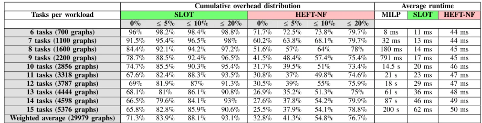
The left-most columns in Table II report, for each workload, the most relevant values for the cumulative overhead distri-bution. This distribution expresses the cumulative probability that an algorithm produces a scheduling with a given overhead, relative to the optimum makespan (calculated by the MILP formulation). The table must be read as follows. Each cell contains the probability that schedules produced for a type of workload (label on the table rows) have an overhead of up to X%, where - is the column’s label. For instance, each cell in the column labeled with 0% contains the probability that an heuristic adds up to 0% overhead, hence a schedule is optimal. For our heuristic (SLOT), optimal schedules are produced for 96% of workloads with 6 tasks, for 91.5% of workloads with 7 tasks and so on up to 65.8% for workloads with 15 tasks. Columns labeled with 10% and 20% are useful to understand performance for moderately constrained systems, i.e., systems where the deadline or time budget falls within 10% or 20% of the optimum makespan. Here, our contribution produces a valid schedule in at least 90% of the cases, for all workloads. By considering a weighted average on all the workloads (last row in Table II, weighted on the number of tasks per workload), we can see that our heuristic returns optimal solutions in the 71.3% of the cases.
To demonstrate the effectiveness of our heuristic with respect to related work, we compared with the Next-Fit version of Heterogeneous Earliest Finish Time (HEFT) [4] heuristic, HEFT-NF. HEFT is commonly used in the literature as a baseline for comparison (see [5], [18]) because of its simplicity and high performance. To the best of our knowledge, a direct comparison with other work is impossible without sensibly denaturing existing heuristics, thus biasing the comparison. On one hand, the works cited in Section II are based on simpler 1D, 2D resource models that are valid for less recent FPGAs, e.g., FPGAs that did not always embed DSPs or on-chip RAM blocks. On the other hand, related works are based on design assumptions that conflict with the context of FPGA-based servers in cloud data centers. For instance, the contribution in [19] is based on partial reconfiguration. In [10], independent tasks are packed, whereas we account for dependencies that partially constrain schedules.
HEFT is a list scheduling algorithm where tasks are scheduled in decreasing order of their upward rank, that is computed based on the critical path (in terms of hardware execution time) from a task to the dependency graph’s sink. HEFT was initially proposed for multi-processor platforms and is directly adaptable to reconfigurable platforms: tasks are assigned to
logical processors (our slots) rather than physical processors.
Many variants of HEFT exist in the literature. We selected the HEFT-Next-Fit as it improves the utilization of logic processors (FPGA slots). In HEFT, if a task C does not fit a logic processor ? because of resource constraints, C and all higher-rank tasks are assigned to another logic processor (a new slot, in our case). In HEFT-NF, instead, ? can execute tasks with higher ranks than C, as long as there are available resources.
Entries in Table II for HEFT-NF have lower values than those for our algorithm. With respect to the latter, thus, HEFT-NF produces good quality schedules with a lower probability. By comparing identical rows for SLOT and HEFT-NF, we can see that the cumulative overhead added by HEFT-NF is distributed further away from the optimum (0% column). Hence, schedules produces by HEFT-NF have more important overheads. On average, last row in Table II, only 32.8% of the HEFT-NF solutions coincide with the optimum.
We can understand the results in Table II by pondering on the criteria used by the heuristics to schedule tasks. Note, that these considerations are valid for the family of HEFT-based algorithms. These algorithms distribute tasks to slots mainly based on the position of a task on a DAG’s critical path. Thus resulting schedules are heavily influenced by a workload’s topology. On the contrary, our heuristic constructs a total order for slots by "cherry picking", at each iteration, the longest task (dominating task), regardless of its location in the DAG. Within each slot, the longer latency of the dominating task hides the shorter latencies of dominated tasks.
To report on worst-case latencies, Fig. 4 shows the cumulative distribution for the weighted average of all workloads (last row in Table II). This average is weighted by the number of graphs per workload. For our heuristic, on average, only 5.36% of all schedules have an overhead above 30% the optimal makespan. In 3 cases, out of 29979, our heuristic adds an overhead equal to 130% the optimal makespan (left top corner in Fig. 4). These extreme cases will be scrutinized to improve the heuristic’s behavior.
The three right-most columns in Table II report the runtime of the MILP formulation, our heuristic and HEFT-NF. These runtimes refer to our Java 8 implementation on a 64 bit Java Virtual Machine, version 1.8.0_201. The computing environ-ment is a workstation with 2 sockets, 16 cores per socket and 64 logical CPUs, at 3.5 GHz. Regardless the quality of our implementation, these runtimes show that HEFT-NF scales better than our heuristic. This is due to the fact that computing candidate slots in our algorithm is more sensitive to increases in the workload’s size. Nevertheless, in absolute terms, they demonstrated SLOT does not have a prohibitively high execution time compared to HEFT-NF, making it
appeal-TABLE II
C .
Cumulative overhead distribution Average runtime Tasks per workload SLOT HEFT-NF MILP SLOT HEFT-NF
0% 5% 10% 20% 0% 5% 10% 20% 6 tasks (700 graphs) 96% 98.2% 98.4% 98.8% 71.7% 72.5% 73.8% 79.7% 8 ms 11 ms 44 ms 7 tasks (1100 graphs) 91.5% 95.4% 96.5% 98% 60.2% 63.8% 68.1% 79.7% 32 ms 13 ms 44 ms 8 tasks (1600 graphs) 84.4% 92.1% 94.2% 97.2% 51.6% 57% 64% 78% 180 ms 14 ms 45 ms 9 tasks (2200 graphs) 78.7% 88.5% 92.4% 96.5% 41.5% 48.4% 57.4% 75.4% 791 ms 17 ms 45 ms 10 tasks (2856 graphs) 74.7% 85.5% 90.3% 95.4% 31.7% 39.5% 51% 73.4% 14.5 s 20 ms 46 ms 11 tasks (3318 graphs) 67.6% 82.4% 88.3% 93.5% 30.8% 37% 49.8% 74.6% 21 s 23 ms 47 ms 12 tasks (3787 graphs) 69% 81.9% 87% 91.3% 30.5% 39% 55% 75.9% 18 s 29 ms 47 ms 13 tasks (4444 graphs) 68.1% 81% 86.1% 90.8% 26.9% 35.2% 51.3% 75% 61 s 36 ms 48 ms 14 tasks (4598 graphs) 66.5% 79.6% 84.1% 93% 27.6% 37.8% 54.2% 79.9% 87 s 46 ms 49 ms 15 tasks (5376 graphs) 65.8% 82.8% 85.9% 90.6% 25.5% 37.9% 54.1% 78.8% 200 s 62 ms 50 ms
Weighted average (29979 graphs) 71.3% 83.9% 88.1% 93.1% 32.8% 41.3% 54.8% 76.7%
Fig. 4. Cumulative distribution of the overhead, for a weighted average of all workloads (last row in Table II).
ing with respect to the expected benefits in the makespan. These runtimes indicate in which scenario our implementation can be used to take scheduling decisions. The relation between an algorithm’s runtime and the frequency at which decisions are needed is the factor that distinguishes between on-line or off-line scenarios.
VI. C
We proposed a new heuristic that schedules tasks in a time-constrained dependency graph to improve the utiliza-tion (profitability) of cloud servers equipped with FPGAs. The formulation of our heuristic is generic and considers :-dimensional models of resources whose requests do not dependent on scheduling choices and are constant in time. We compared our contribution to the next-fit version of the well-known Heterogeneous Earliest Finish Time heuristic (HEFT-NF), that is the best variant of HEFT for FPGAs. In a benchmark of 29979 random dependency graphs, on average, HEFT-NF produces optimal schedules in 32.8% of the cases as opposed to 71.3% for our contribution. SLOT could even be used in scenarios with partial reconfiguration to group tasks into runtime reconfigurable regions. This allows a direct comparison with other contributions such as [19]. Another direction for future work is the efficient inclusion of other resources, especially resources that are independent by the
internal scheduling of each slot but constraints on them can impact on the overall makespan (e.g., energy consumption of tasks, network and memory bandwidth, input/output FPGA resources).
R
[1] J. Weerasinghe, R. Polig, F. Abel, and C. Hagleitner, “Network-attached fpgas for data center applications,” in FPT, 2016, pp. 36–43. [2] S. Hartmann and D. Briskorn, “A survey of variants and extensions of
the resource-constrained project scheduling problem,” Working Paper 02, 2008.
[3] J. Blazewicz, J. Lenstra, and A. Kan, “Scheduling subject to resource constraints: classification and complexity,” Discrete Applied
Mathemat-ics, vol. 5, no. 1, pp. 11 – 24, 1983.
[4] H. Topcuoglu, S. Hariri, and M.-Y. Wu, “Performance-effective and low-complexity task scheduling for heterogeneous computing,” IEEE Trans.
on Par. and Dist. Sys., vol. 13, no. 3, pp. 260–274, 2002.
[5] Y. Qu, J.-P. Soininen, and J. Nurmi, “Static Scheduling Techniques for Dependent Tasks on Dynamically Reconfigurable Devices,” J. Syst.
Archit., vol. 53, no. 11, pp. 861–876, 2007.
[6] S. M. Loo and B. E. Wells, “Task scheduling in a finite-resource, reconfigurable hardware/software codesign environment,” INFORMS J.
on Computing, vol. 18, no. 2, 2006.
[7] J. Teller and F. Ozguner, “Scheduling tasks on reconfigurable hardware with a list scheduler,” in ISPA, 2009, pp. 1–4.
[8] W. Housseyni, O. Mosbahi, M. Khalgui, and M. Chetto, “Real-Time Scheduling of Reconfigurable Distributed Embedded Systems with En-ergy Harvesting Prediction,” in DS-RT, 2016, pp. 145–152.
[9] A. Guillaume, S. Manu, B. Anne, R. Yves, and R. Padma, “Co-scheduling algorithms for high-throughput workload execution,” Journal
of Scheduling, vol. 19, no. 6, pp. 627–640, 2016.
[10] K. Danne and M. Platzner, “Partitioned scheduling of periodic real-time tasks onto reconfigurable hardware,” in IPDPS, 2006, p. 8.
[11] J. chiou Liou and M. A. Palis, “An efficient task clustering heuristic for scheduling dags on multiprocessors,” in Workshop on Resource
Management at IPDPS, 1996, pp. 152–156.
[12] G. C. Buttazzo, Hard Real-Time Computing Systems: Predictable
Scheduling Algorithms and Applications, 3rd ed. Springer, 2011.
[13] K. Danne, R. Mühlenbernd, and M. Platzner, “Server-based execution of periodic tasks on dynamically reconfigurable hardware,” IET Computers
& Digital Techniques, vol. 1, pp. 295–302, 2007.
[14] M. Götz, “Run-Time Reconfigurable RTOS for Reconfigurable Systems-on-Chips,” Ph.D. dissertation, Faculty of Computer Science, Electrical Engineering and Mathematics, University of Paderborn, 2007. [15] M. Götz, F. Dittmann, and C. Pereira, “Deterministic Mechanism for
Run-time Reconfiguration Activities in an RTOS,” in INDIN, 2006, pp. 693–698.
[16] J. Gross, J. Yellen, and M. Anderson, Graph Theory and its Applications, 3rd ed. CRC Press, 2018.
[17] “SLOT evaluation,” https://github.com/SLOTAlgorithm-FPGA, 2020. [18] Y. Shi, Z. Chen, W. Quan, and M. Wen, “A Performance Study of Static
Task Scheduling Heuristics on Cloud-Scale Acceleration Architecture,” in ICCDE, 2019, pp. 81–85.
[19] Y. Qu, J. Soininen, and J. Nurmi, “Using Constraint Programming to Achieve Optimal Prefetch Scheduling for Dependent Tasks on Run-Time Reconfigurable Devices,” in SOCC, 2006, pp. 1–4.
![[PDF] Cours et Exercices php | Télécharger PDF](data:image/gif;base64,R0lGODlhAQABAIAAAP///wAAACH5BAEAAAAALAAAAAABAAEAAAICRAEAOw==)