READ THESE TERMS AND CONDITIONS CAREFULLY BEFORE USING THIS WEBSITE. https://nrc-publications.canada.ca/eng/copyright
Vous avez des questions? Nous pouvons vous aider. Pour communiquer directement avec un auteur, consultez la
première page de la revue dans laquelle son article a été publié afin de trouver ses coordonnées. Si vous n’arrivez pas à les repérer, communiquez avec nous à [email protected].
Questions? Contact the NRC Publications Archive team at
[email protected]. If you wish to email the authors directly, please see the first page of the publication for their contact information.
Archives des publications du CNRC
This publication could be one of several versions: author’s original, accepted manuscript or the publisher’s version. / La version de cette publication peut être l’une des suivantes : la version prépublication de l’auteur, la version acceptée du manuscrit ou la version de l’éditeur.
Access and use of this website and the material on it are subject to the Terms and Conditions set forth at Real Options in Small Technology-Based Companies
Kortner, S.
https://publications-cnrc.canada.ca/fra/droits
L’accès à ce site Web et l’utilisation de son contenu sont assujettis aux conditions présentées dans le site LISEZ CES CONDITIONS ATTENTIVEMENT AVANT D’UTILISER CE SITE WEB.
NRC Publications Record / Notice d'Archives des publications de CNRC:
https://nrc-publications.canada.ca/eng/view/object/?id=23f46ec7-d380-4cd2-9626-866b4d1bc4fe https://publications-cnrc.canada.ca/fra/voir/objet/?id=23f46ec7-d380-4cd2-9626-866b4d1bc4fe
Institute for
Information Technology
Institut de technologie de l’information
Real Options in Small Technology-Based Companies.
Department of General and Industrial Management *
Kortner, S.June 2002
* published in Department of General and Industrial Management, Technical University of Munich, Germany, June 2002, Master's Thesis. NRC 44963.
Copyright 2002 by
National Research Council of Canada
Permission is granted to quote short excerpts and to reproduce figures and tables from this report, provided that the source of such material is fully acknowledged.
Real Options in Small Technology-Based Companies
Stefan Kortner
A thesis submitted to the Department of General and Industrial Management, Technical University of Munich in partial fulfillment of Diplom-Wirtschaftsingenieur.
June, 2002
Munich, Germany
Financial support for this work has been provided by the Institute for Information Technology, National Research Council of Canada.
Abstract
This thesis reports on the results of a research study conducted by the Institute for Information Technology, National Research Council, over the summer of 2001. The study assessed the relevance of an emerging valuation approach known as real options to small technology-based firms. The approach addresses evaluation of investment decisions under uncertainty by viewing a firm‘s ability to respond to changing conditions as a bundle of options that can be exercised at the right time and under the right conditions.
Interviews were conducted with the representatives of the six participating firms, who found the concept of real options appealing.
Systematically scanning different functional areas for possible sources of uncertainty can help identify viable option scenarios in a firm. The functional areas include operations, procurement, R&D, IP management, distribution, sales, after-sales, finance, strategic planning, marketing, and IT infrastructure. Such a methodology can help to reveal opportunities that may otherwise be overlooked or remain implicit.
The scenarios discovered in the firms under study involved staged investments, partnerships with lead customers, patents, arrangements for securing manufacturing capacity, flexible pricing strategies, make or buy decisions, design of a product to allow outsourcing, right to buy out licensed IP, IT infrastructure initiatives, and flexible core technology. Rudimentary quantitative analyses of selected option scenarios confirmed their potential value. Some classical option scenarios reported in the literature were rejected. For example, exit strategies were not deemed viable real options by start-up firms.
The real options terminology can be used to communicate the firm‘s strategy to the stakeholders. This approach can provide firms with a competitive advantage, especially in highly volatile climates.
CHAPTER 1: INTRODUCTION...1
1.1 Motivation ...2
1.2 Contributions and Main Results ...5
1.3 Relevant Work ...5
CHAPTER 2: BACKGROUND ...7
2.1 Basic Option Concepts ...7
2.2 Risk Categories ...8
2.3 Discounted Cash Flow (DCF) ...10
2.4 Decision Tree Analysis (DTA) ...12
2.5 Financial Options...14
2.6 Binomial Model...15
2.7 Migration from Financial Options to Real Options...19
2.8 Recent Applications of Real Options ...23
CHAPTER 3: THE INTERVIEW PROCESS...29
CHAPTER 4: A FUNCTIONAL CLASSIFICATION OF REAL OPTION SCENARIOS ...32
CHAPTER 5: EXAMPLES OF REAL OPTIONS...35
5.1 Production ...35
5.1.1 Securing External Capacity...36
5.1.2 Flexibility for Inputs and Outputs ...37
5.1.3 Scaleability...38
5.4 R&D and Intellectual Property Management ...42
5.4.1 Staged Investments with Exit Options ...45
5.4.2 Patents...47
5.4.3 Standardization ...48
5.4.4 License Buyout Option ...48
5.5 Design Flexibility ...49
5.5.1 Delaying Design Decisions: Different Market Segments ...49
5.5.2 Make or Buy: Special Design for Outsourcing ...50
5.5.3 Flexible Core Technology and Modularity ...50
5.6 Human Resources ...52
5.6.1 Qualifications of Employees...52
5.6.2 Temporary Employment ...52
5.7 Distribution ...52
5.7.1 A New Distribution Channel...52
5.7.2 Inventory...52
5.8 Sales ...53
5.8.1 Customer Acquisition ...53
5.8.2 Pricing Options ...53
5.8.3 Marketing...53
5.9 Valuation of Companies for IPO and M&A...54
CHAPTER 6: NUMERICAL EXAMPLES OF SELECTED OPTION SCENARIOS ...56
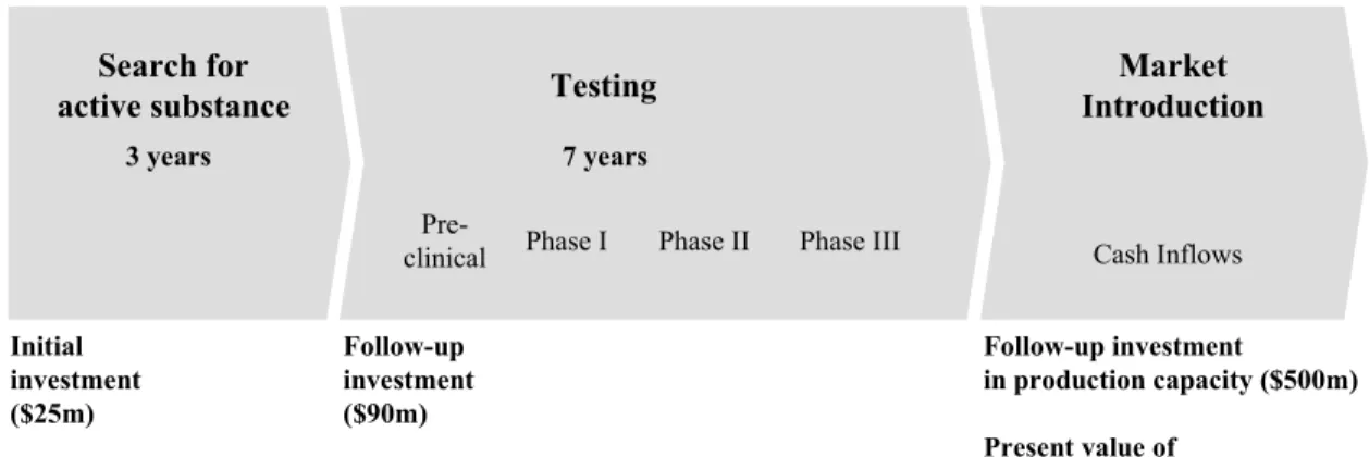
6.1 The Option on Manufacturing Capacity ...56
6.2 License Buyout Option ...60
CHAPTER 7: PRACTICAL LIMITATIONS...63
CHAPTER 8: CONCLUSIONS...64
Chapter 1: Introduction
This thesis explores the applicability of an innovative valuation approach known as real options for the specific needs of small technology-based companies. The real options approach for valuation has advantages over traditional valuation techniques when flexibility in the face of large uncertainty is present. Research in the practical application of real options has been mainly focused on large-scale applications in large companies. This thesis reports on a study that was conducted with six small companies in the high-tech sector to assess if and in what form the real options approach can also be applied in small-technology based companies.
The thesis is organized as follows.
Chapter 1 starts with the motivation for this thesis. The special characteristics of small technology-based companies and their possible requirements for real option analyses are presented next. The main results of this thesis are outlined, and an overview over related literature is given.
The real options approach is explained in Chapter 2 as an innovative valuation technique that can be used both in the strategic planning and in the capital budgeting process of a company. This emerging approach has advantages over traditional techniques like decision tree analysis and discounted cash flow analysis in the treatment of flexibility. These traditional valuation techniques are discussed after a brief overview over different risk categories. Then the binomial option pricing model is explained using the economic principles of replication and arbitrage-free pricing. The challenges arising from the migration of the option pricing model from financial assets to real assets are presented together with possible solutions. The chapter ends with an overview over the current applications of real options.
Chapter 3 describes the interview process with the six participating companies and the lessons learned from the study. The difficulties in finding hidden option scenarios in the interviews have lead to an alternative, functional classification of real options that allows a company to be systematically scanned for possible real option scenarios. The functional classification is outlined in Chapter 4. Numerous examples of real options in small technology-based companies are presented in Chapter 5. The examples are organized according to the presented functional classification, and include some previously unknown
option settings as well as familiar examples from the literature. The valuation of such options is demonstrated in Chapter 6 through two examples that have been discovered.
After some remarks about remaining practical limitations in Chapter 7, the conclusion in Chapter 8 summarizes the results. Numerous hidden options exist in small technology-based companies and these options are a very important part of the business of those firms. The suggested functional option classification has proven to be helpful in the discovery of the option scenarios.
1.1 Motivation
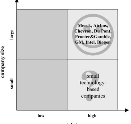
An emerging approach for evaluating investment projects and valuing entire companies stresses the potential of flexibility to create additional value under uncertainty. This approach, known as real options, is considered to be superior to traditional valuation techniques in its ability to capture the value of flexibility. The real options approach argues that flexibility has value if it can be used strategically to react to change. For this reason, the real options approach is theoretically attractive for all companies that operate in highly uncertain environments. These companies are located on the right-hand side in the portfolio in Figure 1.1.
There are important reasons to further distinguish between small and large companies. As the portfolio shows, the real options approach is already employed successfully in some large companies, while evidence of its potential use in small companies is nearly non-existent. Furthermore, academic research in real options has mostly ignored small companies.
One reason for this might be the scale of investments undertaken by large companies. Large scale creates proportionately significant improvement potential, which in turn justifies the extra effort expended on real option analysis. Thus the scale offered by small firms possibly was not deemed as attractive to achieve the desired level of impact. Consequently, most examples of real options have mainly been confined to contexts relevant to large corporations.
?
small technology-based companies uncertainty comp any siz e Merck, Airbus, Chevron, Du Pont, Procter&Gamble, GM, Intel, Biogen la r g e smal l high lowFigure 1.1: Applicability of the Real Options Approach to Different Types of Companies
There might also be a technical reason for the traditional focus on large corporations. The real options approach has its foundations in option pricing theory. Option pricing theory works best for financial assets whose risks are priced in the markets. The connection to the financial markets is usually stronger with large-scale problems because market proxies to the underlying real asset can more easily be found. With decreasing company size and scale, the connection to the financial markets deteriorates. This results in more serious violation of some fundamental assumptions in the valuation of real options.
In addition, small companies lack dedicated finance departments to perform complex valuation tasks. The scarcity and cost of experts prevents them from seeking outside help and exploring new techniques for their strategic planning. Many real option experts work as consultants who target large companies that can afford to pay for their expertise.
Advice is not only scarce, but also ‘mostly aimed at specialists’ 1. The real options literature criticizes that the ‘theory has run ahead of practice’ 2, and that ‘further empirical
work has to be pursued to ensure the practical applicability’ 3.
With this background, it is desirable to analyze and possibly overcome these barriers that have prevented the real options approach to reach smaller companies. Small companies constitute an important and growing part of the economy, and many of them are driven by technological innovation. They operate in highly uncertain environments that suggest the use of the real options approach, and undiscovered options can be expected to exist in these companies.
It has been observed that especially ‘new business ventures have the characteristics of
growth options’ 4 and that the traditional approaches ‘struggle to capture the outstanding
growth prospects’ 5 and potential for shareholder value generation of technology-driven companies. Small technology-based companies have large growth potential, but don’t have the resources for large commitments. They need leverage to grow, this leverage can possibly be provided by options.
Therefore small technology-based companies are promising candidates to participate in a scientific study that aims to broaden the range of applications for real options.
Two questions need to be answered in such a study:
1) Is the real options approach relevant for small technology-based companies? 2) If the answer is yes, then how can existing barriers be overcome?
1 Luehrman (1998), p. 51 2 Dixit and Pindyck (1994)
3 Perlitz, Peske and Schrank (1999), p. 267 4 Willner (1995), p. 221
1.2 Contributions and Main Results
The study has looked specifically for real options within small technology-based companies. The hypothesis that many applications for real options exist has been confirmed. The environment of those small companies is at least as uncertain as the environment of large companies, and small companies have comparable flexibility to react to change as large firms. They also appear to possess growth options, timing options, learning options, and other types of operating options present in large firms. Only the exit option type was generally rejected by small companies because its execution would mean the shut-down of the entire company.
It was observed that small companies are primarily interested in the real options approach as a way of thinking and not so much as an analytical tool for quantitative analysis. They appreciate that the real options approach provides a framework and a language that is able to model and to communicate important business issues. The interest in quantitative analysis concentrates mainly on occasions when a company licenses or sells a technology, because the options associated with that technology can be part of the deal.
Progress was also made in the methodology to identify option scenarios. The small companies that participated in the study had difficulties to relate to the popular option examples of large companies. They need to be offered examples of options that are closer to their own business. Scanning the company’s functional departments (e.g. production, R&D, distribution...) for choices to react upon uncertainty has been a successful way to suggest as well as to identify option settings. The discovered option examples are sorted and presented according to the new functional classification for two reasons. First, these examples show the relevance of the real options approach for small technology-based companies. Second, they can serve as templates that help other small companies to look for similar options in their own business. By employing this new, and ‘user-oriented’ methodology, a major barrier to the wider adoption of the real options approach – the identification of options – can be overcome.
1.3 Relevant Work
In a recent study, Triantis and Borison (2001) have identified and interviewed 34 companies that are using the real options approach. The study gives a good overview over
the current practical use of the real options approach. The companies belong to differrent industries that have large uncertainties and high investments in common. Apparently all of the companies are quite large. There is no evidence for the use of real options in smaller companies.
The study of Triantis and Borison also reports that different companies are attracted by different features of the real options approach. Some companies are interested in real options as an analytical tool, others understand the approach as a way of thinking that allows to frame and communicate investment decisions, others have included the approach in the organizational planning process to identify flexibility. These features could be also presented to smaller companies as reasons to use the real options approach. The recommended procedure to introduce the real options approach to a company is via a pilot project.
Hommel (1999) presents a comparison of different valuation techniques and shows the benefits of using option pricing for investments under uncertainty. He draws on the analogies of real options to financial options (uncertainty, flexibility, irreversibility) to identify possible real option settings in business.
Luehrman (1998) recognizes the uniqueness of most business opportunities and thus the difficulty of finding option settings. He also notes that most of the input data for a real options calculation are available from traditional discounted cash flow analyses so that the additional effort for calculating an option is low.
There is a wide agreement in the literature about the classification of options. Hommel (1999), Amram and Kulatilaka (1999), Perlitz, Peske and Schrank (1999), among others promote a classification of options according to the type of flexibility they provide (e.g. exit options, timing options). Especially Perlitz, Peske and Schrank give a good overview over other distinctive criteria of options (e.g. discrete/continuous price movements, traded/not traded underlying). These categories are very helpful to choose the appropriate mathematical option model, once the option itself is identified. Amram and Kulatilaka state that uncovering real option scenarios has been difficult.
A comprehensive introduction into the real options approach can be found in the textbook of Trigeorgis (1996).
Chapter 2: Background
2.1 Basic Option Concepts
The real option approach builds on the formula discovered for the pricing of financial options. A financial option gives its holder the right but not the obligation to buy (or to sell) a certain amount of a financial asset in the future for a pre-determined price (called the strike price). The holder of the option will execute the option only if it is profitable, that is, when the market price is high. Otherwise, the option will be forgone. By this choice, the payoff function with respect to different market prices is no longer linear. The maximum loss is limited to the amount that was initially paid for the option (the option premium). The resulting payoff function typically has the form of a hockey stick and is shown in Figure 2.1.
stock value option
value
C
0
strike price spot price option
premium
Figure 2.1: The non-linear payoff function (‘hockey stick’)6
The valuation of such an option to determine a fair option premium had been considered an unsolved problem for decades until the nobel-prize-winning work of Black, Merton and Scholes solved the problem in the early seventies. These three financial economists found an analytical solution to the value of a call option (the price to be paid to acquire an option to buy an asset) based on a standard model of asset price dynamics and on replication and no-arbitrage-arguments.
6 Chatterjee and Ramesh (1999), p. 2
Later it was noticed that certain types of investments in real assets have similar non-linear payoff functions as financial options. These non-linearities result from managerial flexibility that can be taken advantage of to limit losses while retaining full upside potential of a business. The valuation of business opportunities with non-linear payoffs can be enhanced by the use of option pricing techniques. When option pricing techniques are employed correctly, the calculated option value represents the value of embedded flexibility. The more uncertain the economic and business environments are, the more valuable is flexibility.
Consider an intuitive example of a plane ticket. Usually, a plane ticket can not be refunded if the passenger gets ill and misses the flight. If the passenger already suspects that he might get ill, he may want to buy a refundable ticket instead. Thereby he would limit his loss in the case of illness. The choice to give back the ticket enhances its value, therefore it will be more expensive. The price difference is the value of the option to get the ticket refunded.
Similar options occur in strategy planning and in the capital budgeting process of companies. Whenever managerial flexibility is identified to react to an uncertain future, application of option pricing techniques and the underlying thinking to valuation of real assets could be used to capture the additional value of the flexibility. “Used properly, the real options
approach can identify important sources of value that are often missed or de-emphasized by the traditional DCF approach” 7. Majd and Pindyck maintain that the application of modern financial theory leads to a better microeconomic foundation for investment behavior8.
2.2 Risk Categories
A brief discussion of risk is helpful for understanding the limitations of the traditional valuation techniques. These will be explained in the later chapters.
Risk is the exposure to uncertainty. Most investors are risk-averse, in that they would take extra risks only if they are sufficiently rewarded. Investors require a higher return for a stock whose returns are more uncertain than a government bond that pays out income tied to a
7 Faulkner (1998), p. 50
fixed interest rate. The rate of return of an asset with minimal or no risk is called the risk-free rate. It represents the minimum rate of return required of any investment. This rate can be observed in the markets. For example in the U.S., the risk-free rate is determined by the yield of short-term government bonds or treasury bills. This benchmark parameter will be denoted by r.
By definition, other forms of investments bear higher risks. The returns on stocks of certain public companies, for example, are very uncertain. Therefore investors require higher returns on risky stocks than on safer investments. This forces the companies to earn at least the required return, relative to other assets in the market.
Several models establish a relation between risk and return. One of the most well-known
models is the Capital Asset Pricing Model (CAPM)9. The model decomposes risk into
systematic and unsystematic components. The systematic component of risk affects all assets in the market, the unsystematic component affects only individual assets. According to CAPM, the expected return of an asset is proportional to the systematic risk of that asset, that is the component that affects all assets in the market. Since investors can diversify away unsystematic, or private risk, CAPM maintains that capital markets do not reward bearing private risk. This position in turn influences the choice of the proper rate of return, or discount rate, for valuing risky investments. CAPM is adopted throughout this thesis as the underlying model for selecting the proper discount rate in any quantitative analysis.
Even in the traditional valuation techniques like Discounted Cash Flow (DCF) and Decision Tree Analysis (DTA), the treatment of risk is a complicated problem that presents itself in the selection of a proper discount rate. The discount rate is used to transform future cash flows to present values and should reflect the cost of the employed capital. Because the capital markets do not reward private risk, companies should use a discount rate that reflects only the systematic component of risk present in a business.
It may however be inappropriate to use a single discount rate even within a single project. The actual level of risk may vary substantially in the different phases of a project (for example
in research, development, commercialization)10. Risk often declines in later phases, resulting in excessive risk-adjustments when the discount rate is kept constant throughout the entire business case.
2.3 Discounted Cash Flow (DCF)
The advances in understanding how capital markets work and how risky assets are valued have been transferred to capital budgeting techniques. In particular, Discounted Cash Flow analysis is a widely used technique that has been derived from finance theory11.
‘DCF spreadsheets are at the heart of most corporate capital-budgeting systems’ 12. A survey in the year 1994 showed that 95% of the participating companies indicated that DCF analysis was either very important or somewhat important in getting a project accepted13.
‘The fundamental idea of the discounted cash flow approach is that the value of a project is defined as the future expected cash flows discounted at a rate that reflects the riskiness of the cash flow’ 14. The discount rate should take into account the systematic risk of the cash flows, that is the extent to that cash flows are correlated with the market as a whole.
Discounted cash flow analysis involves two steps:
1. Coming up with the best estimate of the cash flows over a time horizon
2. Discounting these expected cash flows back to the present time at a risk-adjusted discount rate.
The result of a DCF analysis is also called the Net Present Value (NPV). The formula for calculating the NPV is:
10 Hodder and Riggs (1985) 11 Myers (1984), p. 126 12 Luehrman (1998), p. 51 13 Flatto (1996), p. 2
(
k)
I C NPV T t t t − + =∑
=1 1Ct = forecasted cash flow for period t
T = project lifetime
k = opportunity cost of capital I = investment required at t = 0
The NPV rule says that a project should be executed if its net present value is greater than zero. If all alternative projects have positive NPVs then the alternative with the highest NPV should be chosen.
‘The discounted cash flow method has become the standard for valuing bonds, stocks and other fixed-income securities. It is especially sensible for relatively safe stocks which pay regular dividends’ 15.
DCF analysis applied to a company or project valuation makes an implicit assumption concerning the expected scenario of cash flows. DCF analysis can evaluate only the actual cash flows a project is expected to yield, not taking into account any flexibility that might influence the cash flows.
‘DCF analysis does not explicitly recognize that managerial flexibility has a value’ 16. It usually ‘underestimates investment opportunities because it ignores management’s flexibility
to alter decisions as new information becomes available’ 17.
Therefore DCF is not as helpful in valuing companies with significant growth opportunities like technology start-ups. ‘The DCF approach is likely to be more useful for cash cows than
for growth businesses with substantial risk and intangible assets’ 18.
15 Myers (1984), p. 134
16 Benaroch and Kauffman (2000), p. 200 17 Flatto (1996), p. 2
The importance of choosing an appropriate valuation method is underlined by the statement that ‘an uncritical acceptance of the sometimes subtle implications of DCF can lead
the way into strategic error’ 19.
2.4 Decision Tree Analysis (DTA)
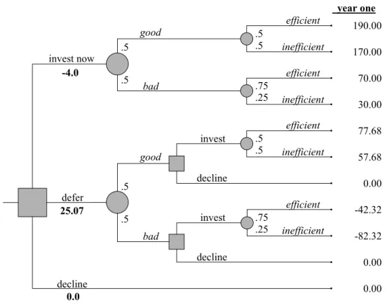
‘The decision tree analysis helps management to structure a decision problem by mapping out all feasible alternative actions over time contingent on uncertain events in a tree-like manner’ 20. It provides a significant conceptual improvement over the way that DCF analysis handles uncertainty and flexibility21. A decision tree like the example in figure 2.2 shows the expected payoffs that are contingent on future states of the environment and on future decisions of the management.
19 Faulkner (1998), p. 50
20 Trigeorgis and Mason (1988)
-104.00 190.00 -104.00 170.00 -104.00 70.00 -104.00 30.00 0.00 77.68 0.00 57.68 0.00 0.00 0.00 -42.32 0.00 -82.32 0.00 0.00 0.00 0.00
project cash flows current year one
invest now defer decline good bad good bad decline decline invest invest efficient inefficient efficient inefficient efficient inefficient efficient inefficient .25 .75 .5 .5 .5 .5 .25 .75 .5 .5 .5 .5 -4.0 25.07 0.0
Figure 2.2: Example of a Decision Tree22
Branching can occur in the tree either in form of an event node to map out different outcomes of the environment or in form of a decision node that represents a specific decision. To each branch a probability is associated. Many large companies maintain a database of past projects that aid with probabilistic estimates23. To solve the decision tree, the calculation is started at the terminal date, recursively computing the expected payoffs while choosing the best decisions. The Net Present Value, incorporating the benefits of flexibility, is the value associated with the root of the tree.
The main shortcoming of DTA is the problem of determining the appropriate discount rate to be used in working back through the decision tree. The flexibility represented in each decision node is equivalent to an option. By this flexibility, the probability distribution of the projected payoffs is changed. ‘A single discount rate cannot be used since asymmetric claims
22 Smith and Nau (1995), p. 804 23 Boer (2000), p. 3
on an asset with limited downside risk and unlimited upside risk do not have the same expected rate of return as the underlying asset itself’ 24.
The adjustment of the discount rate according to the probability distribution is accomplished by option pricing techniques. Therefore option pricing is claimed to be superior to decision tree analysis if DTA is applied naively25. If both option pricing and decision analysis are applied correctly, they must give consistent results26.
2.5 Financial Options
A discussion of financial options will help to understand how real options work. A financial option gives its holder the right, but not the obligation, to buy or sell a financial asset before or on a specific day for a predetermined price, called the strike price. An option to buy an asset is referred to as a call option. A put option gives its holder the right to sell an asset. The asset on which the option is written or based is called the underlying. If the exercise of the option is only possible at the expiration date in the future, the option is called a European option. If the exercise is possible at any time until the expiration date, the option is called an American
option.
The holder of an option always has the choice to exercise the option or not. In advance, it is not possible to tell whether the option will be exercised or not, because this decision is contingent on the value of the stock in the future, which is uncertain. In some cases the exercise of the option will be profitable, in some other cases the exercise would lead to a loss. For example, the exercise of a call option will be profitable if the future market price of the asset is higher than the strike price. In this case the option would be exercised. If the future market price falls below the strike price, exercise would lead to a loss, so the option would expire worthless.
24 Chatterjee and Ramesh (1999), p. 2 25 Copeland, Koller and Murrin (1990) 26 Smith and Nau (1995), p. 795
For several reasons, options have been introduced to the financial markets. Speculation, which is often associated with options or derivatives, is only an inevitable side-effect. Options can be used as an insurance against price uncertainty of stocks. For example, the holder of a stock of a public firm can buy a put option on that stock, allowing him to sell this stock for a floor price if the stock value drops sharply. Options can also act as an insurance against drops or raises in foreign currencies. Their main feature is a non-linear payoff, limiting downside potential while maintaining full upside potential. The maximum loss is limited to the purchasing price of the option. Options can also be thought of as levered positions on the underlying asset. For example, one can synthesize a call option by partly financing the purchase of the underlying asset through a risk-free loan. In turn, options have greater financial risk than the underlying asset.
Options have value because they give the holder a chance on some future profits. The practical calculation of the option value remained impossible until the path-breaking work of Black, Merton and Scholes in the early seventies. Several economic insights and arguments were linked together which allowed for the valuation of standard financial options. ‘The
breakthrough in option pricing theory resulted in a valuation technique that circumvented the need to estimate risk-adjusted discount rates for financial options’ 27. The technique was adopted soon as a possible tool for valuing contingent claims due to the deficiencies of existing techniques28.
2.6 Binomial Model
Each option is written on an underlying asset. The future payoff of the option depends on the future price of the asset. Therefore, the current price of the asset and estimates about its future development are very important inputs for option pricing. Models of option pricing typically begin with the specification of how the prices of the underlying assets evolve over
27 Triantis and Borison (2001), p. 12 28 Lindt and Pennings (1997), p. 84
time. The objective is then to identify the price of an option, taking the behavior of the underlying process as a given29.
The formula of Black and Scholes is a closed-form solution that computes the value of a European call option. It assumes that the value of the underlying asset follows a lognormal
diffusion process, or Geometric Brownian Motion. The binomial model can be viewed as a
discrete-time approximation of the Black and Scholes model. The binomial model is easier to understand and more suitable for modeling complex options30. McGrath emphasizes that the underlying asset on that the option is written must be priced, and that this price must be known31.
Suppose that the underlying asset is the stock of a public firm. The current stock price is denoted S. Its value is known because it can be observed in the financial markets. After one period, the stock can have only two possible prices. The higher price is denoted by S+, the lower price by S-. The ratio of S+ to S is called the upward factor, denoted by u, and the ratio of S- to S is called the downward factor, denoted by d.
In reality, the stock can assume an infinite number of possible prices after one period. By linking several binomial periods together, more realistic distributions of the stock price can be created.
The volatility σ is a measure of the total risk of the stock. It can be used to capture the uncertainty surrounding the price movement. The volatility is usually estimated using historical performance data of the stock. For the binomial model, a valid combination of u- and d-factors can be computed according to
σ
e
u= and
u d = . 1
Then, the development of the underlying stock from the beginning to the end of the period can be written as
29 Sundaram (1997), p. 85
30 Cox and Ross and Rubinstein (1979), p. 229f 31 McGrath (1997), p. 975
S d S S u S S ⋅ = ⋅ = − +
At the end of the period, the net payoff of the option conditional on its exercise is the stock price minus the strike price. If the payoff is negative, the option will not be exercised and its future value becomes zero, thus creating a nonlinear payoff function.
The future values of the option are denoted by C+ and C-, and its present value by C.
) 0 , max( ) 0 , max( X S C X S C C − = − = − − + +
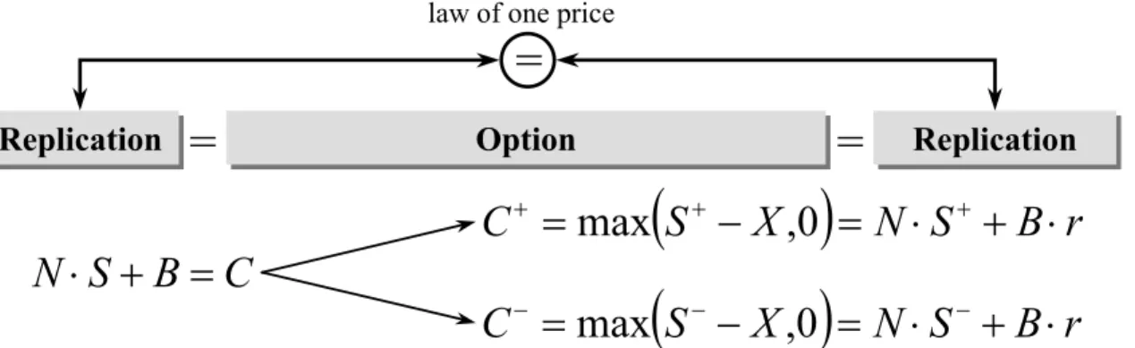
When the two possible developments of the stock, S+ and S-, and the strike price X are known, then the future option values C+ and C- are also known. To calculate the present value of the option C, two economic arguments can be used: replication and the law of one price (no arbitrage).
In the binomial model, it is always possible to find a portfolio of primitive securities that exactly replicates the option’s payoffs at any state. This portfolio consists of the underlying stock itself and of a risk-free asset, such as a bond or a risk-free loan. These two securities are sufficient to complete the market. There are two possible states of the world and two linearly independent securities. ‘Every risky cash flow can be represented as a linear
combination of the payoffs of these two securities’ 32. The value of the bond develops with the risk-free interest rate r. Its present value is set equal to one, after one period it will have the value r. The development of the stock is also assumed to be known in the binomial model. If the future value of the portfolio is known, its present value is also known. Then, by the law of one price, the current option value C must be identical to the present value of the replicating portfolio. ‘This procedure is economically correct in that it is guaranteed to deliver
arbitrage-free prices’ 33.
The components of the replicating portfolio, the number of the shares of the stock and the amount borrowed in the risk-free bond, need to be further specified. Let N denote the number
32 Smith and Nau (1995), p. 799 33 Black, Fischer and Scholes (1973)
of units of the underlying stock to buy and B the amount to be borrowed at the risk-free rate. The replication ties the value of the portfolio to the option value, the law of one price serves as a bridge from the future values to the present value. Figure 2.3 illustrates this solution.
(
S
X
)
N
S
B
r
C
+=
max
+−
,
0
=
⋅
++
⋅
(
S
X
)
N
S
B
r
C
−=
max
−−
,
0
=
⋅
−+
⋅
C
B
S
N
⋅
+
=
OptionOption ReplicationReplication
Replication
Replication
=
=
=
law of one price
Figure 2.3: Option Pricing by Replication and the Law of One Price
In this formula, three variables are unknown: C, N and B. Therefore, three equations are needed to solve for the unknowns. These three equations are:
r B S N C r B S N C B S N C ⋅ + ⋅ = ⋅ + ⋅ = ⋅ + = − − + +
Solving these equations yields for the unknown C:
r C d u u r C d u d r C − + ⋅ − + − + ⋅ − − =
This formula can be rewritten as:
(
)
r C p C p C − ++ − ⋅ ⋅ = 1 by introducing: d u d r p − − = and d u u r p − + − = − ) 1 ( .If the upward and downward factors fulfill the condition d < r < u to prevent arbitrage, then p and (1-p) are greater than zero and less than one, so they have the properties of a probability. The measures p and 1-p are called the risk-neutral probabilities (or also martingale measures), because they would be equal to the actual probabilities if the investors
were risk-neutral. Using the risk-neutral probabilities enables a test of consistency in model specification, because inconsistently specified models permit arbitrage opportunities. An arbitrage opportunity represents a free lunch, the creation of something out of nothing. ‘It can
be shown that a model of option pricing is complete if, and only if, the model admits exactly one risk-neutral probability’ 34.
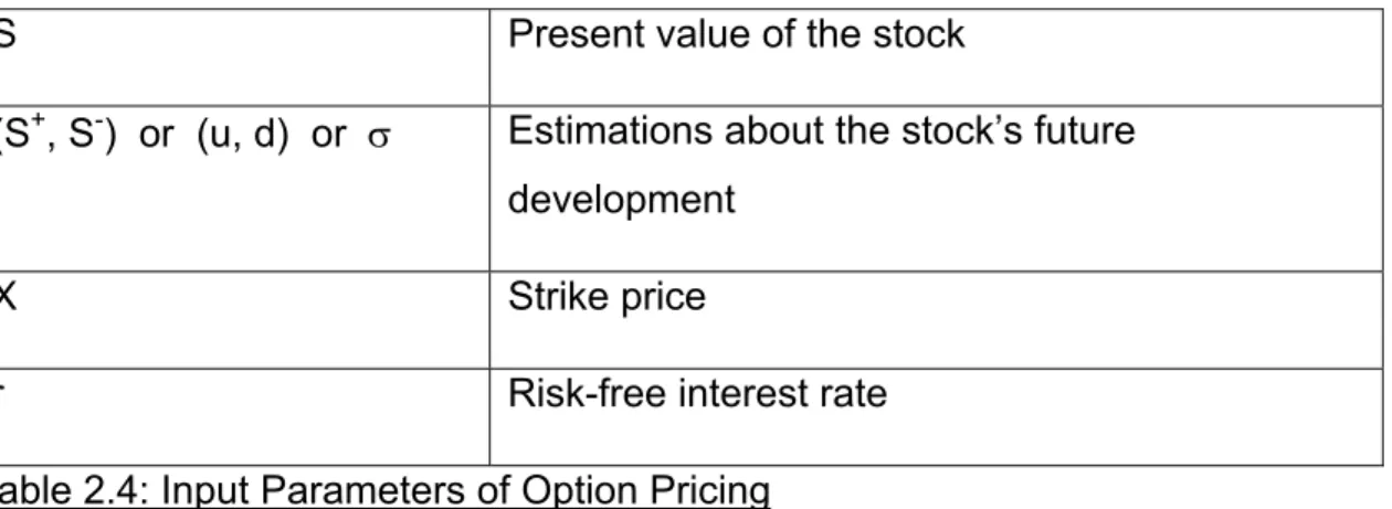
Hence the option pricing using the binomial model relies on the input parameters shown in Table 2.4.
S Present value of the stock
(S+, S-) or (u, d) or σ Estimations about the stock’s future development
X Strike price
r Risk-free interest rate
Table 2.4: Input Parameters of Option Pricing
For financial options, these input data can be either observed or estimated easily. The present value S of the stock can be observed in the financial markets because stocks are traded continuously. The strike price X can be chosen deliberately, so once it is chosen, it is also known. The risk-free interest rate r can be observed as the yield of short-term government bonds. For the future stock development, historical data of the stock prices can provide a sufficient estimate of the volatility.
2.7 Migration from Financial Options to Real Options
The technique to value financial options can also be used to value real options. While financial options are written on an underlying financial asset, a real option is based on an underlying real asset. Similar to a financial asset, the future value of the underlying real asset is uncertain. The first examples of real options were found in businesses where the underlying real assets are close to the market. Financial assets are traded, that means that a current
34
price can be observed in the markets, as well as a series of historical prices from which the volatility σ of the asset can be derived. The financial markets are also assumed to be efficient, which means that all available information about the future development of the asset is already reflected in the market price. Real assets that behave very much like financial assets are for example the right to drill for crude oil (that is correlated with the future oil price), and real estate. Oil is traded in a market, thus a spot price and information about its volatility exists. Real estate is also traded, meaning that the market attaches a price to it. Information about the future prices is also already included in the spot prices. For example, if it was believed that the future oil price will rise because of a shortage, the spot price will also rise accordingly. The closeness to the market of some real assets enable the application of option pricing techniques to option-like situations in these businesses. For example, once an oil field has been developed, the oil price can be relatively high so that exploration is profitable. The oil price could also be so low that exploration would lead to a loss. In this case, the oil company would choose not to exploit the oil and to wait until the oil price has climbed again. The liberty to choose between exploiting and not exploiting is valuable because it protects the company from losses due to the uncertain price of oil. The value of this option would be impossible to capture with traditional DCF analysis. It can be calculated using option pricing techniques and added on top of the DCF to compute a total value of the oil field development.
Since these early examples, the option pricing techniques have spread into other businesses, where the behavior of the underlying assets diverge from traded financial assets. New popular applications of real options are in research and development, with the idea that a newly developed technology leads to the option to develop a product. The developed product itself gives the option to market it in the case that markets are favorable. Here, the underlying assets have different properties than financial assets. ‘A striking problem that
arises from the observation that the underlying asset of a real option is non-traded concerns the estimation of the volatility of the underlying asset. In contrast with financial options, there are no historic time series that enable to estimate the uncertainty of the underlying asset’ 35. For example, the underlying of an option to market a new product is the revenue based on the market volume. If the demand and thus the market volume is high, it will be profitable to launch the new product. If the demand is low, the product will not be launched. To model the
35
underlying, the present value of the future market volume with its volatility must be estimated. These values are sometimes very hard to estimate, because the underlying is not traded. Two techniques are used to find estimates for the volatility, known as spanning and hotelling36.
‘The so-called spanning duplicates a non-traded asset by a twin security’ 37. The twin security is also often called a proxy. It is a traded asset or a portfolio that is highly correlated with the actual underlying. Such a portfolio is called a tracking portfolio because it tracks the volatility of the target market. The pharmaceutical company Merck uses its own stock volatility as a proxy for the volatility of the NPV of future cash flows resulting from new products38. For the option to wait before developing land, real estate companies use data on land transactions to get an estimate of the volatility39. Other businesses opportunities, especially technology-based projects, are unique, so the likelihood of finding a similar asset is low40. In these cases, hotelling can be used.
‘Hotelling Valuation is to estimate the market potential for the product and then try to evaluate this potential and use it as the underlying’ 41. The expected value of the underlying can be found in the traditional DCF spreadsheets that are commonly prepared to evaluate investment proposals42. The minimum and maximum boundaries of the future values of the underlying are explicitly estimated, using judgements of the senior management to attain reasonable values for the uncertainty43. In complicated cases, the estimation can be aided by
36 Perlitz and Peske and Schrank (1999), p. 259 37 Pindyck (1993) 38 Nichols (1994) 39 Quigg (1993) 40 Luehrman (1998), p. 52 41 Sick (1989) 42 Luehrman (1998), p. 51
a Monte Carlo simulation that synthesizes a probability distribution function for project returns44.
Then, still an estimate for the discount rate is needed to bring the uncertain future values back to the present. The discount rate has to reflect the riskiness of the underlying, more precisely the systematic component of its risk. It is argued that any spreadsheet that computes NPV already contains the information necessary to compute S (and X)45. This is correct if a proper discount rate has been used.
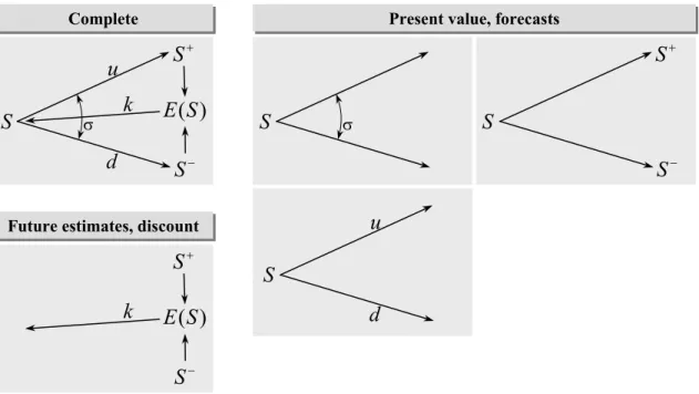
In different real-world settings, different data can be collected. Sometimes this data is not exactly what option pricing techniques require as an input. The data needs to be transformed into the input parameters of the option calculation. For example, Figure 2.5 gives an overview over different sets of input parameters that are sufficient for the binomial model.
+ S − S S k E(S) u d σ Complete Complete S u d + S − S S S σ
Present value, forecasts
Present value, forecasts
+ S − S ) (S E k
Future estimates, discount
Future estimates, discount
Figure 2.5: Relations between Alternative Input Parameters of the Binomial Model
In the upper left corner, the relationships among alternative input parameters are shown. If only some of them are known, the rest can sometimes be calculated. In some cases the present value of the underlying S and forecasts about the future are available. This is the
44 Luehrman (1998), p. 58 45 Luehrman (1998), p. 53
case for example with stock options. The present value S can be observed in the stock market, and the historic volatility gives an estimate about the future volatility σ. Under the assumption of lognormal diffusion46, knowing σ is equivalent to knowing the upward factor u and the downward factor d of the binomial model. With these factors, the future values of the underlying S+ and S- can be calculated. These three cases of knowing the present value and having estimates about the future are equivalent and can be interchanged.
The situation is more complicated if no present value can be directly observed. In all real option applications that are not based on traded underlying assets, a discount rate k is needed to calculate the present value. This is especially true for real options in small technology-based companies. It is the same problem as in the calculation of the DCF. A practicable way is to start with the expected future value of the underlying E(S). This estimate will be readily available from sales forecasts for example. ‘It is assumed that unbiased
estimates of cash flows are provided. Clearly, this assumption is also used in all discounted cash flow studies’ 47. The next step is to estimate the best case S+ and the worst case S- of the future value of the underlying. Hotelling and spanning does not work in this case because they start from the present value, which is not known in this case. Therefore explicit assumptions about S+ and S- need to be made. Then, a discount rate k is needed to calculate the present value. The discount rate should reflect the market risk of the underlying asset.
2.8 Recent Applications of Real Options
The field of applications for the real options approach has been continuously expanded in the last years. One of the earliest and most popular examples was found in the oil industry, only a few years after the publication of the option pricing formula by Black, Merton and Scholes in 1973. A lease on land provides the option to drill for oil. ‘If an exploration project is
successful, a company has the option to drill wells and pump oil. If the project doesn’t pan out, the company has the option to cease development and cut its losses. The option increases the value of the exploration project because it protects the full potential gain of the
46 Cox, Ross and Rubinstein (1979) 47 Lindt and Pennings (1997), p. 85
investment while reducing the possible losses’ 48. Another early example was the valuation of gold mine reserves that provide the option to extract gold if the gold prices are favorable49. These first examples of real options were appealing because of their close proximity to the financial markets. In these examples, ‘the value of the underlying asset depends on price
movements of natural resources’ 50. This means practically that the prices are observable in markets. The present value can be used directly as an input for the option pricing formula, the historical development of the price can be used to compute the volatility. After more than two decades of application, the real options approach is not limited anymore on projects based on natural resources. Although the first examples remain very popular, applications in other industries have been found. The viewpoint that ‘current applications of real options mainly
concern investment projects dependent on natural resources’ 51 is being outdated by many examples from the high-tech sector.
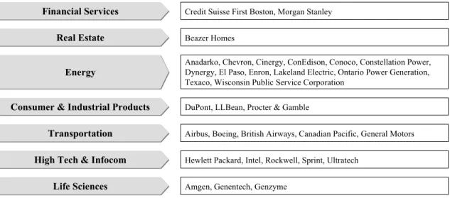
Examples of real options have been found in many industries and in many different settings. Figure 2.6 gives an overview over industries in which the real options approach is already used, with examples of companies that participated in a recent real options survey52.
48 Amram and Kulatilaka (1999) 49 Brennan and Schwartz (1986) 50 Brennan and Schwartz (1985) 51 Lindt and Pennings (1998), p. 3 52 Triantis and Borison (2001)
Energy
Energy
Anadarko, Chevron, Cinergy, ConEdison, Conoco, Constellation Power, Dynergy, El Paso, Enron, Lakeland Electric, Ontario Power Generation, Texaco, Wisconsin Public Service Corporation
Financial Services
Financial Services Credit Suisse First Boston, Morgan Stanley
Real Estate
Real Estate Beazer Homes
Transportation
Transportation Airbus, Boeing, British Airways, Canadian Pacific, General Motors
High Tech & Infocom
High Tech & Infocom Hewlett Packard, Intel, Rockwell, Sprint, Ultratech
Life Sciences
Life Sciences Amgen, Genentech, Genzyme
Consumer & Industrial Products
Consumer & Industrial Products DuPont, LLBean, Procter & Gamble
Figure 2.6: Companies using Real Options
The energy sector is very comparable to the oil industry because natural resources are used as a source of power, and on the other side the energy is traded in a market where energy prices can be observed. The observation of prices is also possible for real estate. The pharmaceutical industry is already using real option models frequently in capital budgeting53. The return of a new drug is highly uncertain and calls for innovative valuation techniques. One of the pioneering companies in that industry is Merck54. The pharmaceutical industry can be seen as a sector of the more general life sciences industry. There are also examples from the transportation industry, consumer and industrial products, and high-tech industries.
All of these industries have in common that large investments need to be made, and that the returns are very uncertain. The expansion of the real options approach into engineering-driven industries was favored by the experience and history of these companies in the internal use of analytic tools55.
The following list gives an impression of the abundance of possible option settings. If not noted otherwise, the examples are taken from Trigeorgis (1996).
• Property rights are an option to extract mineral reserves.
53 Axel and Howell (1996) 54 Nichols (1994)
• A patent gives the option to develop a new product.
• In a production facility, the option to expand can be contained. By making an additional investment outlay higher revenues can be obtained.
• Building a plant with lower initial construction costs and higher operating costs creates the flexibility to contract operations by cutting down on operating costs if the product turns out to do worse than initially expected.
• Some productions offer the possibility to shut down the production or not to operate temporarily if the cash revenues are not adequate to cover the variable costs of operating. This represents a call option on that year’s cash revenue, the exercise price is the variable cost of operating.
• Option value can exist in the ability to terminate a project, selling the assets on the secondhand market for their salvage value.
• Flexibility in inputs (electricity, gas) and outputs (chemicals) of a facility can contribute to its value.
• An acquisition of an unrelated company can be undertaken for the sake of optional access to an new market.
• A research project, if successful, provides at completion the opportunity to acquire the revenues of the developed, commercialized product upon incurring a production outlay. • If a lead customer gives a guarantee to purchase or a guarantee on minimum prices, the
probability distribution of the payoffs becomes nonlinear, reducing risk.
• Corporate liabilities can be viewed as call or put options on the value of the firm.
• Outsourcing a project transfers the risk of a project failure to other parties, reducing downside risk and creating a nonlinear payoff.56
• Option valuation can be used to calculate how much to spend on lobbying, thereby actively changing the boundary conditions of an option.57
56 Benaroch and Kauffman (1999)
It has been observed that although real options appear in a large number of settings, ‘they
tend to take a limited number of forms’ 58. The literature has established a classification of real options that distinguishes among timing options, growth options, staging options, exit options, flexibility options, operating options, and learning options59.
• Timing options give the flexibility to choose a favorable time for a decision.
• Growth options provide a company with the strategic chance to expand into new markets or businesses.
• Staging options are created by dividing long-term projects into phases. After each phase, the option to continue will be exercised if the previous phase was successful.
• Exit options act like an insurance. They provide the chance to sell off an unprofitable business for its salvage value.
• Flexibility options give the choice between different inputs and outputs of a production process.
• Operating options in a production process give the ability to shut down a production temporarily or to change the production volume in favorable and unfavorable times.
• Learning options can be used to defer a project or an investment to wait for the arrival of new information for a better decision.
This classification has been made according to the type of the management’s reaction upon the uncertainty. It helps to communicate the idea of real options to the management because frequent decisions of the management are addressed.
Although the real options approach originated from the pricing of financial options, the calculation of an option value is not the only way real options are used in companies. A recent
57 McGrath (1997), p. 974f
58 Amram and Kulatilaka (1999), p. 96 59 Amram and Kulatilaka (1999), p. 96
survey60 has identified three purposes for which the real options approach is used in different companies.
1. Real options can be understood as a way of thinking. In these cases, real options are primarily used as a language that frames and communicates decision problems qualitatively.
2. Real options are used as an analytical tool. The option pricing models are mainly used to value projects with known and well-specified optionality.
3. Real options are included as a part of the organizational process. Real options are used as a management tool to identify and exploit strategic options.
The survey also reports on the relevance of the real options approach:
‘For the great majority of firms, real options is not viewed as a revolutionary solution to new business conditions. Instead, it is seen as part of an evolutionary process to improve the valuation of investments and the allocation of capital, thereby increasing shareholder value. The adoption of these techniques is viewed as providing a competitive advantage through better decision-making. For other firms, real options is perceived as a dramatic departure from the past that has the potential to alleviate important concerns, manage critical business risks, or reveal exciting growth opportunities’ 61.
60 Triantis and Borison (2001), p. 6 61 Triantis and Borison (2001), p. 4f
Chapter 3: The Interview Process
Several small technology-based companies were asked to participate in the study underlying this thesis. At the time of the interviews, all of the companies were in the beginning of their lifecycle and had not yet reached their maturity or market saturation. They pioneered technologies that had just left research stage or entered the commercialization stage.
Therefore, in each company a significant amount of uncertainty about the future could be expected. A series of interviews was held with six such companies. The purpose of these interviews was to introduce the real options approach to the companies, and to assess the relevance of the approach for each company.
The initial interview strategy consisted of five steps:
1. Present a simple and intuitive option example to communicate the concept. 2. Explain uncertainty and flexibility as preconditions for options.
3. Ask for option scenarios within the company. 4. Solve the option scenarios.
5. Present the results to the company and obtain feedback.
A variety of key people from each company were addressed. Their acceptance and knowledge of the real options approach and their understanding of it varied widely. The idea and purpose of real options and of option pricing was found to be very difficult to communicate to technically oriented people. The middle management was more ready to accept the concept of real options. People from the top management (CEO, CFO) had mostly already heard about option pricing. Especially CFOs were mostly already familiar with the well-known Black-Scholes formula in the context of financial options.
As a first step, the interviewed people were presented a basic and intuitive example of real option valuation, followed by the explanation of uncertainty and flexibility.
Purely technically oriented employees tended to challenge the real options approach. This was also helpful for the study, because it showed main points of criticism that can be held against the real options approach, which needed to be clearly addressed if the real option approach was to become more popular. In particular, the interviewees asked what
advantages the real options approach has over established techniques. The interviewer explained that DCF doesn’t capture the value of future decisions based on uncertainty at all. DTA is able to include future decisions, but it needs to be pointed out that the naïve DTA always uses the same discount rate for the payoffs, which might be wrong. In this sense, option pricing should be explained as an ‘economically corrected decision tree analysis’, that takes into account that risk changes over time, and that the discount rate also varies.
Another critical question was the purpose and relevance of employing real options. The ultimate answer to this question must lie in the making of improved decisions. The decisions will be tied closer to the financial markets, allowing ‘a more accurate valuation of alternatives
and thus more educated decisions in the face of uncertainties’ 62. But besides quantitative valuation, the real options approach was also explained as a way of thinking, providing appropriate vocabulary to frame and communicate important parts of a decision under uncertainty. Also, the real options approach can be embedded in the managerial process to look specifically for chances within uncertainties.
The top and middle management did not challenge the real options approach at all. The benefits of real options were clearly understood and readily accepted, but here the obstacle was a different one. After hearing the initial basic example of a real option, the most common response was that the example was appealing, but that similar situations did not exist within their own companies.
The first interviews revealed that the companies need to be offered a finer grid of option examples. In the follow-up interviews they were shown a known classification of possible real options examples, categorized according to their impact on business (growth options, time-to-build options, options to defer, options to change scale, options to switch input or output, and exit options). This classification was an attempt to suggest templates to relate to. It was not helpful in discovering option scenarios, because the option examples in this classification were relevant mostly for large corporations in specific industries, such as real estate, natural resources and pharmaceutical, and did not capture typical problems of small, technology-based companies. For example, the exit option was consistently received as a kind of “suicide” strategy, and therefore rejected. Large companies are able to dispose of a single
project and re-allocate the resources easily, but for small start-up companies that often focus on a specific product or product line, failure is not an option.
Thus it became evident that existing templates or examples of real options did not appeal to small technology-based companies. Moreover, the companies were obviously not yet ready to identify option scenarios by themselves. Therefore a different methodology of screening for option scenarios that suited better to the context of the companies under study, was needed.
To get an insight into the biggest uncertainties and the most difficult decisions of the companies, the interviewees were asked about their historic development path. Then, this information was used to form hypothetical option scenarios, which were presented to the companies. Even if these suggested options did not actually exist, they were closer to the companies’ businesses than the previously mentioned examples from oil and pharmaceutical companies. They helped to direct the companies’ attention to specific topics and to discover true real option scenarios. For example, a chip-design company without manufacturing facility was presented the hypothetical option to build such a facility. It was assumed that the company could build a facility at any future time whenever it would be profitable. The option would be executed if demand was high, and the option would simply expire if there was enough free capacity in other facilities. Again, this suggestion reflected the situation of a large semiconductor company, overlooking the fact that the price of a new factory could easily exceed billions of dollars, thus making this option unfeasible for small startup-companies with limited access to financial resources. But this example turned the discussion to the capacity problem, which was indeed an important question for the young company. Further questions in this topic lead to the discovery of the capacity option.
This discovery also showed that the right examples and templates that appeal to the companies can be very helpful in the future screening for option scenarios. This observation lead to an alternative classification of real options.
Chapter 4: A Functional Classification of Real Option Scenarios
There is still much discussion on whether the real options approach will gain wide popularity or not. It is argued that even the NPV rule took many years to become established in the corporate practice. To become widely used, mainstream real options have to be useful not only for a handfull of companies, but for a larger and more diverse corporate population. Almost all of the real option examples today are found in large companies with large-scale problems. These examples do not reflect the typical situations of smaller firms.
The first step is to identify real options. ‘Up to date, uncovering real option scenarios is
difficult’ 63. The basic approach is usually starting with an existing example and trying to find similar situations. Consequently, finding a new option involves an element of luck. Thus, existing examples need to be structured and illustrated in a way that is relevant to the context of the target organization.
The necessary preconditions for an option scenario are the existence of uncertainty and of a choice, a contingent decision. To structure real option scenarios, one possible way is to look for common sources of uncertainty that apply to most of the companies. Many examples in the literature locate the uncertainty in the target markets of a company. Market uncertainty applies to almost all companies. The companies’ reaction to it will be individual and can be structured according to defer, switch, growth and exit opportunities. More recent examples have located uncertainty within research, also with a large portion of final market risk. Following the question of different sources of risk, other answers are also possible. On the input side of a company, opposite to its sales markets, are the procurement markets. The insight that more sources of uncertainty exist opens the door to a completely new classification of options, according to the functional origin of uncertainty. Examples of options in procurement already exist. The optional plane orders from Boeing are an example of contractual options in procurement. These procurement options are promising applications of real options when prices of procured assets can be observed in the markets.
As more examples will be discovered, this functional map can be expanded. It can serve as a reference to companies that attempt to manage and make most out of their optionality.